NNETFIX: An artificial neural network-based denoising engine for gravitational-wave signals

Abstract

Instrumental and environmental transient noise bursts in gravitational-wave detectors, or glitches, may impair astrophysical observations by adversely affecting the sky localization and the parameter estimation of gravitational-wave signals. Denoising of detector data is especially relevant during low-latency operations because electromagnetic follow-up of candidate detections requires accurate, rapid sky localization and inference of astrophysical sources. NNETFIX is a machine learning-based algorithm designed to remove glitches detected in coincidence with transient gravitational-wave signals. NNETFIX uses artificial neural networks to estimate the portion of the data lost due to the presence of the glitch, which allows the recalculation of the sky localization of the astrophysical signal. The sky localization of the denoised data may be significantly more accurate than the sky localization obtained from the original data or by removing the portion of the data impacted by the glitch. We test NNETFIX in simulated scenarios of binary black hole coalescence signals and discuss the potential for its use in future low-latency LIGO-Virgo-KAGRA searches. In the majority of cases for signals with a high signal-to-noise ratio, we find that the overlap of the sky maps obtained with the denoised data and the original data is better than the overlap of the sky maps obtained with the original data and the data with the glitch removed.

1 Introduction

The field of GW (GW) astronomy began with the first direct detection of a GW signal from a BBH (BBH) merger [1] on September 14^th, 2015. Nine additional BBH mergers were detected with high confidence during the first and second LIGO [2] and Virgo [3] observation runs [4]. During the third LIGO-Virgo observation run, 39 binary merger events were detected with high confidence [5], including two exceptional BBH events [6, 7, 8] and a possible NSBH (NSBH) merger [9].

On August 17^th, 2017, the first detection of a GW signal from a BNS (BNS) merger, GW170817, expanded multi-messenger astronomy to include GW observations [10]. A short GRB (GRB) was detected approximately 1.7 seconds after the BNS merger time [11]. The sky map calculated from the GW signal allowed the identification of the event with an EM (EM) counterpart [10, 11]. The association of this GW event with the observed EM transients supports the long-hypothesized model that at least some short GRB are due to BNS coalescences [12] and has provided many insights into fundamental astrophysics and cosmology. In April 2020, a second BNS merger without an EM counterpart was detected [13].

In order to detect GW signals, ground-based GW detectors must be extremely sensitive, causing them to become highly susceptible to instrumental and environmental noise [4]. In particular, transient noise bursts, or glitches, may impair the quality of detector data. The presence of a glitch in the proximity of a GW signal can adversely affect the analysis of the latter, including calculating the sky localization of the source. The most notable example of such an occurrence was GW170817, where the effect of a glitch was mitigated in low-latency by removing the contaminated portion of the data and in follow-up studies by applying ad hoc mitigation algorithms [10, 14].

One possibility to mitigate the effect of a contaminating glitch would be to discard the data from the affected detector. This is the simplest and fastest solution; however, it is also likely to impact the analysis and sky localization, especially in cases where data is only available from two detectors. Another technique that can be used in low-latency is gating, which removes the data affected by the glitch. One method of gating is to set the data affected by the glitch to zero using a window function to smoothly transition into and out of the gate [15]. Gating was used in the case of GW170817 to produce the low-latency sky localization for EM follow-up observations [16]. On larger latencies, glitch mitigation techniques such as using BayesWave [17] to model and subtract the glitch can be used [16].

Figure 1 shows an example of the detrimental effect gating data can have on the sky localization error region of a simulated BBH merger signal. The sky localization obtained with the gated data significantly differs from the sky localization estimated from the full data. Also, the 90% sky localization error region after the gating is applied no longer includes the true sky position of the injected signal.

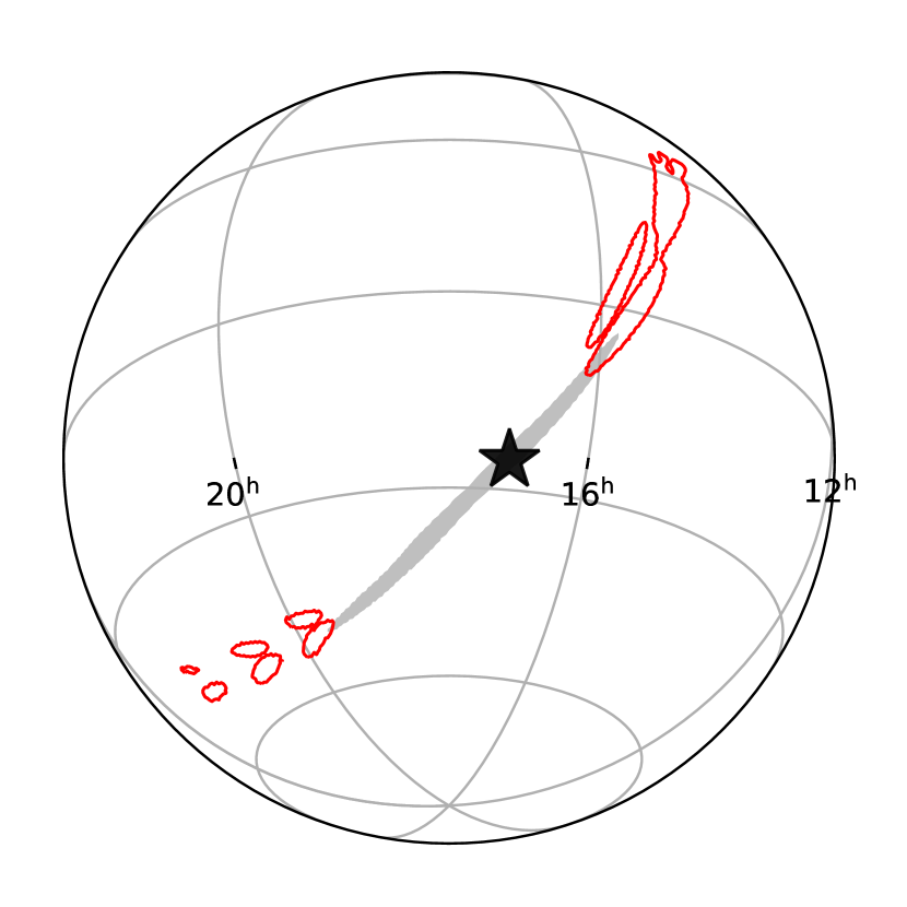
Figure 1: Left: Whitened time series of a simulated BBH signal with two-detector network SNR $\rho_{\rm N}=42.4$ and component masses $(m_{1},m_{2})=(35,29)$ $M_{\odot}$ in aLIGO recolored Gaussian noise (red curve). A 130 ms gate is applied 30 ms before the geocentric merger time (gray curve). The vertical black-dashed line denotes the merger time in H1. Right: The 90% sky localization error regions from the full data (gray area) and the gated data (red empty contours). The star indicates the true sky position of the simulated signal.

The higher detector sensitivity of LIGO and Virgo in their third observing run has led to an increased number of GW candidate detections from different astrophysical populations [6, 13, 9]. Future observation runs with higher sensitivity are expected to produce even greater detection rates, which would lead to higher chances of observing GW signals contaminated by glitches. The inability to accurately estimate the sky localization of GW candidates with potential EM counterparts due to glitches contaminating the signal could put at risk new astrophysical discoveries such as those made with GW170817. Thus, the development and implementation of accurate low-latency denoising methods could be highly beneficial to multi-messenger observations.

In this paper, we present a machine learning-based algorithm to denoise transient GW signals called NNETFIX (“A Neural NETwork to ‘FIX’ GW signals coincident with short-duration glitches in detector data”). NNETFIX uses ANN to estimate the portion of a signal which is lost due to the presence of an overlapping glitch. We train the ANN to reconstruct the portion of a gated signal on a template bank of BBH waveforms injected into simulated noise data. The accuracy of the algorithm is assessed by comparing the recovered waveform, SNR (SNR), and sky map from the processed data to the corresponding quantities obtained before gating. We derive a set of statistical metrics to assess the improvement in these quantities.

2 Algorithm implementation, training and testing

We consider a scenario in which a transient BBH GW signal is observed by a network of at least two detectors and the data of one detector is partially gated to remove a glitch. Without loss of generality, we perform the analysis for the two LIGO detectors, H1 (H1) and L1 (L1), with the gating applied to data from the H1 detector. We assume the merger time at the geometric center of Earth (or geocentric merger time) to be (approximately) known from L1 data. We denote with $s_{f}(t)$, $s_{g}(t)$ and $s_{r}(t)$ the full time series, the gated time series, and the NNETFIX reconstructed time series, respectively. The output of NNETFIX can be thought of as the map

$$s_{r}(t):=F\left[s_{g}(t)\right]\,.$$ (1)

We train an ANN regression algorithm to construct the map $F$ such that $s_{r}(t)\sim s_{f}(t)$. The NNETFIX implementation uses the scikit-learn [18] MLP (MLP) Regressor, a type of ANN in which the nodes (mathematical functions) are arranged into layers and connected to every node in the preceding and/or succeeding layers [19]. Each node calculates a weighted linear combination of the outputs from the preceding layer and applies an activation function that introduces a non-linearity into the node’s output. The ANN trained by NNETFIX consists of one hidden layer containing 200 neurons. In the ANN training process, NNETFIX uses the rectified linear unit (ReLU) activation function [20] and the ADAM stochastic gradient-based optimizer [21] with a learning rate of $10^{-3}$. Ten percent of the training data samples are set aside and used for validating the training. The training iteration stops if the ANN performance plateaus with a tolerance level of $10^{-4}$ to avoid overtraining. To reconstruct the gated portion of the time series, one hidden layer works better than multiple hidden layers for the loss function of mean square error and the number of hidden layers tested. The values from the loss function have a weak dependency on the number of neurons.

To train the algorithm, we first build template banks of simulated non-spinning IMRphenomD BBH merger waveforms [22] with varying intrinsic and extrinsic parameters. To reduce the potential for overtraining, each template bank also includes a number of (pure) noise time series. We distribute the positions of the injected signals isotropically in the sky. The waveform coalescence phase, polarization angle, and cosine of the inclination angle are uniformly distributed in the intervals $[0,2\pi]$, $[0,\pi]$, and $[-1,1]$, respectively. We uniformly distribute the network SNR $\rho_{\rm N}$ [15] of the simulated signals in the range $[11.3,42.4]$. We consider three distinct template banks corresponding to low, medium, and high BBH component masses to assess the prediction accuracy of the trained ANN for different signal lengths. The BBH component masses are uniformly sampled according to a Jeffreys prior for the matched-filter detection statistic. As the mass of the system decreases, we employ a higher number of templates to properly cover the mass parameter space [23, 24, 25, 26].

For each of the three distinct template banks, we build 12 TT (TT) sets: first, we inject each waveform into 50 distinct realizations of recolored Gaussian noise for aLIGO (aLIGO) at design sensitivity; second, we include the (pure) noise time series; third, we shuffle and split the set by 70%–30% for training and testing; and finally, we apply the 12 combinations of gate durations $t_{d}=$ (50, 75, 130) ms and gate end-times before the geocentric merger time $t_{e}=$ (15, 30, 90, 170) ms. The time series are sampled at 4096 Hz, whitened, and high-passed. A conservative value of 25 Hz is used for the high-pass filter. The gates are implemented as a reversed Tukey window with a taper of 0.1 s and held fixed with respect to geocentric merger time; however, the merger time seen in the H1 detector naturally shifts due to the sky position and the polarization angle of the GW signal. Table 1 shows the range of the component masses, the number of waveforms, the number of noise series, and the dimension of the sets for the different scenarios.

	$m_{1}$ [$M_{\odot}$]	$m_{2}$ [$M_{\odot}$]	$n_{s}$	$n_{n}$	Set dimension ($n_{s}\times 50+n_{n}$)
Low	10–15	8–12	348	1900	19300
Medium	15–25	12–18	251	1350	13900
High	28–42	23–35	61	300	3350

Table 1: Component mass ranges, number of waveforms ($n_{s}$), number of pure noise series ($n_{n}$), and dimension of the TT sets for each of the three scenarios and combinations of gate durations and end-times.

We test the effectiveness of the ANN by calculating the coefficient of determination for the MLP Regressor in scikit-learn on the testing sets [18]. The coefficient of determination ranges from $-\infty$ (bad) to 1 (perfect estimation), with positive values corresponding to some degree of accuracy. We evaluate the coefficient of determination on each testing set after training the ANN on the corresponding training set. The ranges of the coefficient of determination for the testing sets are [0.773, 0.882], [0.750, 0.883], and [0.691, 0.879] for the low-mass, medium-mass, and high-mass scenarios, respectively, and the means are 0.833, 0.827, and 0.814.

We test for potential statistical effects in the training method by considering the medium mass scenario with a gate duration of 50 ms and a gate end-time of 30 ms as a representative case. For 100 trials, we find that the coefficient of determination ranges from 0.800 to 0.826 with a mean of 0.815, which is consistent with the ranges of the testing sets.

The effect of NNETFIX on quantities such as SNR and sky localization varies for different component masses, network SNR, and gate settings. Therefore, we construct 108 additional independent exploration sets with fixed network SNR $\rho_{\rm N}=(11.3$, 28.3, $42.4)$ and component masses of (12, 10), (20, 15), (35, 29) $M_{\odot}$, and identical combinations of gate durations and end-times as the TT sets. Each exploration set consists of 512 independent time series with the remaining parameters distributed as in the TT sets.

3 Performance in the time-domain

NNETFIX’s performance in estimating the full time series can be assessed by computing the amount of SNR lost in the reconstruction process. We define the FRS (FRS)

$$\text{FRS}=\frac{\rho_{f}-\rho_{r}}{\rho_{f}}\,,$$ (2)

where $\rho_{f}$ and $\rho_{r}$ are the (single interferometer) peak SNR of the full time series and the reconstructed time series in H1, respectively. Positive values of FRS close to zero generally indicate accurate time series reconstructions. However, FRS $\sim 0$ may also occur when the gating does not significantly reduce the peak SNR of the full series, and thus, $\rho_{f}\sim\rho_{g}\sim\rho_{r}$. These cases can be separated by the FSG (FSG)

$$\text{FSG}=\frac{\rho_{r}-\rho_{g}}{\rho_{g}}\,,$$ (3)

where $\rho_{g}$ is the peak SNR of the gated series. The FSG characterizes the amount of SNR gained by the reconstructed time series in comparison to the gated time series. Typically, NNETFIX performance is better for smaller values of FRS and larger values of FSG.

Median values of FRS across the exploration sets range from FRS $=-0.09$ (high-mass case with $\rho_{N}=11.3$, $t_{d}=170$ ms and $t_{e}=50$ ms) to FRS $=0.22$ (medium-mass case with $\rho_{N}=28.3$, $t_{d}=15$ ms and $t_{e}=130$ ms). Sets with smaller gate durations are generally characterized by lower FRS values. All exploration sets with $t_{d}=50$ ms have FRS $<0.1$. The fraction of sets with FRS below this threshold reduces to 0.78 and 0.55 for gate durations of 75 ms and 130 ms, respectively. Similarly, exploration sets with gates that are farther away from the time of the merger also tend to have a lower median value of the FRS. All sets with gate end-times at 170 ms before merger have median FRS $<0.07$ while only 81%, 55% and 11% of the samples with $t_{e}=90$, 30 and 15 ms have FRS below this threshold, respectively. The effects of the network SNR and component masses on FRS are less significant. About 83% of the sets with $\rho_{N}=11.3$ have median FRS $<0.1$ compared to 75% for the sets with $\rho_{N}=28.3$ and $\rho_{N}=42.4$. The percentages of low-mass, medium-mass and high-mass sets with FRS $<0.1$ are comparable at about 78%, 75% and 81%, respectively.

Median values of FSG range from $\sim 0.02$ (low-mass, low-SNR case with $t_{d}=170$ ms and $t_{e}=50$ ms) to $\sim 0.89$ (high-mass, low-SNR case with $t_{d}=130$ ms and $t_{e}=15$ ms). High-mass (low-mass) exploration sets are typically characterized by higher (lower) values of the FSG. All high-mass sets have FSG $>0.08$, while all low-mass sets have FSG $<0.07$. Gate end-time and SNR do not seem to significantly affect the value of FSG. The gate duration has a larger effect. Sets with longer gate durations typically have larger median value of the FSG. Two thirds of the sets with $t_{d}=130$ ms have FSG $>0.08$ compared to only 42% of the sets with $t_{d}=50$ ms.

A combined threshold of FRS $\gtrsim 0$ and FSG $\gtrsim 0.01$ is a conservative choice for good reconstructions. About 70% of the samples across all the exploration sets satisfy this criterion. Figure 2 shows the NNETFIX data reconstruction for the time series of Fig. 1. As shown in Fig. 3, the reconstructed time series recovers a large signal energy in the gated portion. In this case, FRS $=0.05$ and FSG $=0.53$.

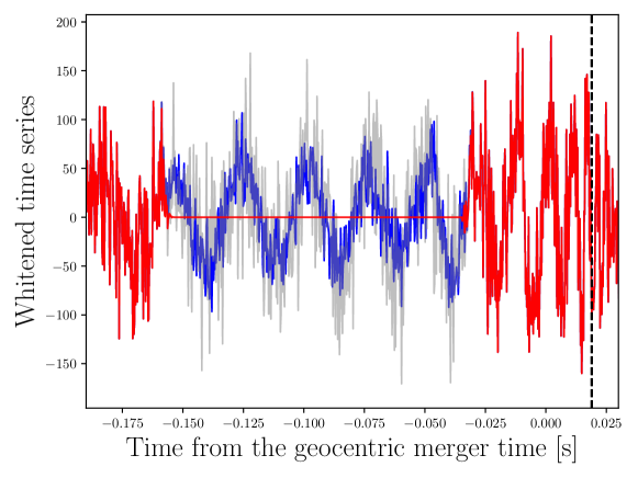
Figure 2: The whitened full time series (gray), the gated time series (red) and the reconstructed time series (blue) for the simulated event of Fig. 1. The vertical black-dashed line denotes the merger time in H1.

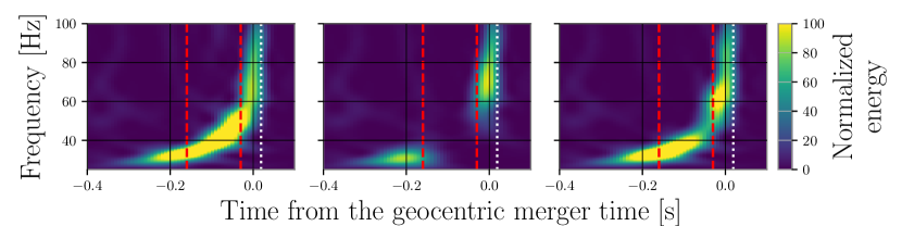
Figure 3: Time frequency representations of the full (left), gated (middle), and reconstructed (right) time series for the simulated event of Fig. 2 using the Q transform [27]. The vertical red-dashed line denotes the gate and the vertical white-dotted line denotes the merger time in H1.

A complementary metric to evaluate the performance of the algorithm is the FMG (FMG)

$$\text{\acs{FMG}}=\frac{M_{r}-M_{g}}{M_{f}-M_{g}}\,,$$ (4)

where the match $M_{i}$ between a time series $s_{i}$ and the injected waveform $h$ is

$$M_{i}=\frac{\langle s_{i}|h\rangle}{\sqrt{\langle s_{i}|s_{i}\rangle\langle h|h\rangle}}\,.$$ (5)

The inner product of two time series $s_{i}$ and $s_{j}$ is defined as

$$\langle s_{i}|s_{j}\rangle=4\Re\int^{f_{N}}_{f_{1}}\frac{\tilde{s_{i}}(f)\tilde{s_{j}}^{\ast}(f)}{S(f)}df\,,$$ (6)

where the tilde indicates the Fourier transform, the star denotes the complex conjugate, $S(f)$ is the detector noise PSD (PSD), $f_{1}$ is the high-pass frequency, and $f_{N}$ is the Nyquist frequency.

In Eq. (4), we assume $M_{f}-M_{g}>0$. In rare instances (0.5% of all exploration set data samples), $M_{g}$ becomes larger than $M_{f}$. This occurs for small values of the single interferometer peak SNR (median value of 4.6) when the gated portion of the data is dominated by noise and anti-correlates with the injected waveform. In the following, we remove these data samples from the exploration sets.

The FMG assesses how well the NNETFIX reconstructed data matches the signal in comparison to the full data and gated data. Positive (negative) values of the FMG correspond to $M_{r}$ greater (smaller) than $M_{g}$, indicating that the NNETFIX reconstructed time series has a better (worse) match with the injected waveform than the gated time series. Values of the FMG larger than 1 indicate that the ANN overfits the data, i.e., the reconstructed time series is more similar to the injected waveform than the full time series. Therefore, we consider the reconstructions with $0<\text{\acs{FMG}}\leq 1$ to be successful. Figures 4 and 5 show the distributions of the FMG for two exploration sets from the medium-mass scenario. Figure 6 displays the comparison of these distributions.

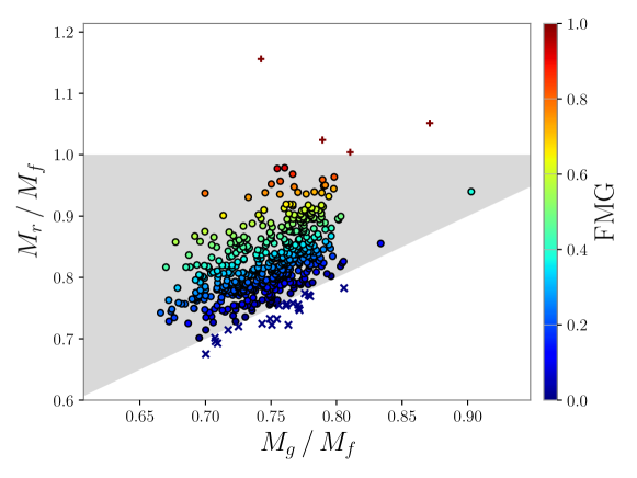
Figure 4: Scatterplot of $M_{r}/M_{f}$ vs. $M_{g}/M_{f}$ for the exploration set with $\rho_{N}=42.4$, $(m_{1},m_{2})=(20,15)$ $M_{\odot}$, $t_{d}=130$ ms and $t_{e}=30$ ms. The circles denote samples with $0<\text{\acs{FMG}}\leq 1$, the $\times$ markers denote samples with FMG $\leq 0$ and the $+$ markers denote overfitted samples with FMG $>1$. The gray area denotes the region of the parameter space with $0<\text{\acs{FMG}}\leq 1$, which contains 95% of the reconstructed time series. Two outliers with values FMG$=-0.4$ and FMG$=1.6$ are not shown in the plot in order to improve readability.

Figure 5: Scatterplot of $M_{r}/M_{f}$ vs. $M_{g}/M_{f}$ for the exploration set with $\rho_{N}=11.3$, $(m_{1},m_{2})=(20,15)$ $M_{\odot}$, $t_{d}=130$ ms and $t_{e}=30$ ms. The circles denote samples with $0<\text{\acs{FMG}}<1$, the $\times$ markers denote samples with FMG $\leq 0$ and the $+$ markers denote overfitted samples with FMG $>1$. The gray area denotes the region of the parameter space with $0<\text{\acs{FMG}}\leq 1$, which contains 59% of the reconstructed time series.

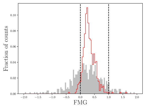
Figure 6: Distribution of the FMG for the exploration sets with component masses $(m_{1},m_{2})=(20,15)$ $M_{\odot}$, gate duration $t_{d}=130$ ms, gate end-time $t_{e}=30$ ms, and $\rho_{N}=11.3$ (gray-filled) and $\rho_{N}=42.4$ (red). The vertical dashed lines denote FMG$=0$ and FMG$=1$. The efficiency of the set with $\rho_{N}=11.3$ is 59%. The efficiency of the set with $\rho_{N}=42.3$ is 95%.

We quantify NNETFIX’s performance by estimating the reconstruction efficiency, which we define as the fraction of successfully reconstructed samples, i.e., samples with $0<\text{\acs{FMG}}\leq 1$. The fractions of samples with FMG $\leq 0$, $0<\text{\acs{FMG}}\leq 1$ and FMG $>1$ for all exploration sets are given in Tables 4-4. The efficiency across all exploration sets varies from approximately $0.31$ to over $0.95$. There is a mild dependence on the component masses of the system; the median value of the efficiency decreases from $0.77$ for the low-mass scenario to $0.61$ for the high-mass scenario when all other parameters (SNR, gate duration and gate end-time) are held fixed.

Within each mass scenario when the gate duration and gate end-time are held fixed, NNETFIX’s efficiency typically improves by a factor $\sim 1.5$–2 as the network SNR increases. As the SNR becomes higher, the algorithm can rely on a larger amount of signal energy before and after the gated portion of the data to reconstruct the time series. NNETFIX successfully reconstructs over two thirds of the time series with $\rho_{N}=28.3$ or larger for all low-mass and medium-mass exploration sets and over half of the time series for the high-mass sets with the exception of two marginal cases with gate duration $t_{d}=75$ ms and gate end-time $t_{e}=90$ ms. The exploration sets with $\rho_{N}=11.3$ exhibit lower efficiencies, ranging from 31% for the high-mass set with $t_{d}=75$ ms and $t_{e}=90$ ms to 66% for the low-mass set with $t_{d}=130$ ms and $t_{e}=15$ ms.

Figure 7 shows the efficiency for the exploration sets with component masses $(m_{1},m_{2})=(20,15)M_{\odot}$ as a function of the single interferometer peak SNR. The percentage of successful reconstructions ranges from $\sim$ 33%–66% at low peak SNR to $\gtrsim$ 80% at high peak SNR, with the lowest values $\lesssim$ 40% occurring for the sets with $t_{d}\geq 75$ ms and $t_{e}\geq 30$ ms. Time series with peak SNR above $\sim$ 20 show successful reconstructions in 70% or more of the cases, irrespective of gate duration and end-time.

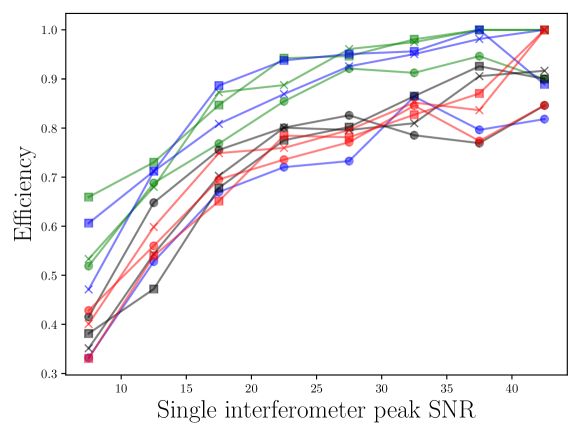
Figure 7: Efficiency as a function of the single interferometer peak SNR for the scenario with component masses $(m_{1},m_{2})=(20,15)$ $M_{\odot}$. Each line corresponds to a different gate duration and gate end-time combination. Green (blue, black, red) markers denote gate end-times $t_{e}=15$ (30, 90, 170) ms. Circles (crosses, squares) denote gate durations $t_{d}=50$ (75, 130) ms. The bin width is 5.

Changing the gate duration does not seem to have a significant effect on NNETFIX’s efficiency, which only varies slightly at fixed network SNR and gate end-time across all exploration sets. Similarly, for fixed gate duration and network SNR, the gate end-time before merger time also has a marginal effect, although NNETFIX tends to produce better reconstructions when the gate is closer to the merger time, especially for long gate durations in the low-mass and medium-mass scenarios.

In conclusion, we find that NNETFIX may successfully reconstruct gated data of durations up to a few hundreds of milliseconds and as close as a few tens of milliseconds before the merger time for a majority of time series with single interferometer peak SNR greater than 20.

4 Performance of sky maps

The NNETFIX reconstructed time series are expected to produce better sky maps, and therefore better sky localization error regions of the astrophysical signal, than the gated time series. We evaluate this improvement by comparing the overlaps of the sky map derived from the full time series with the sky maps derived from the gated time series and the reconstructed time series. In the following, we generate the sky maps with a modified version of a pyCBC [28] script, pycbc_make_skymap, in which the data can be manually gated.

We follow Ref. [29] and define the overlap of two sky maps (1,2) as

$$O_{1,2}=\frac{\displaystyle 4\pi\int\!p_{1}(\Omega)p_{2}(\Omega)\,\mathrm{d}\Omega}{\displaystyle\int\!p_{1}(\Omega)\,\mathrm{d}\Omega\int\!p_{2}(\Omega)\,\mathrm{d}\Omega}\,,$$ (7)

where $p_{1}(\Omega)$ and $p_{2}(\Omega)$ are the sky localization probability densities of the sky maps and the integrals are over the solid angle $\Omega$. The discretized version of Eq. (7) is

$$O_{1,2}=N\sum_{i=1}^{N}P_{1i}P_{2i}\,,$$ (8)

where $P_{1i}$ and $P_{2i}$ each denote the sky localization probability of the $i$-th pixel of the corresponding sky map, and $N$ is the total number of pixels. Each sky map is normalized such that the sum of the pixel values over the entire map is 1. Equation (8) gives values in the range $(0,N)$. Higher values of $O_{1,2}$ indicate a better overlap between the two maps while lower values denote worse overlaps and/or maps which tend to have less-localized error regions.

A suitable metric to evaluate the improvement in the sky localization of a signal due to NNETFIX’s reconstruction is the ORL (ORL)

$$\text{\acs{ORL}}=\log_{10}\frac{O_{r,f}}{O_{g,f}}\,,$$ (9)

where $O_{r,f}$ ($O_{g,f}$) denote the overlaps of the sky maps obtained with the reconstructed (gated) time series and the full series. Positive (negative) values of the ORL indicate that the sky map from the reconstructed time series has a larger (smaller) overlap with the sky map from the full time series than the latter has with the sky map from the gated time series. Tables 7-7 give the fraction of samples with positive ORL for all exploration sets.

High values of the ORL are obtained when the overlap of the reconstructed (gated) sky map with the sky map from the full time series is large (small). The former typically occurs for reconstructed time series with large values of the FMG. The latter may happen when the loss of signal due to the gate is high and even small gains in the single interferometer peak SNR have a significant impact on the sky localization.

An example of the ORL distribution as a function of $O_{g,f}$ is shown in Fig. 8 for the exploration set with $\rho_{N}=42.4$, component masses $(m_{1},m_{2})=(20,15)$ $M_{\odot}$, $t_{g}=130$ ms and $t_{e}=30$ ms. The median value of the ORL is $1.14^{+1.15}_{-1.10}$, where the error is a 1-$\sigma$ percentile. The ORL is positive in 87% of the samples. Median values of ORL for all exploration sets are given in Tables 10-10.

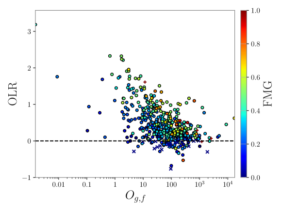
Figure 8: Scatterplot of ORL and $O_{g,f}$ for the 512 samples from the exploration set with $\rho_{N}=42.4$, component masses $(m_{1},m_{2})=(20,15)$ $M_{\odot}$, gate end-time $t_{e}=30$ ms and gate duration $t_{d}=130$ ms. The colored circles denote samples with $0<\text{\acs{FMG}}\leq 1$, the $\times$ markers denote samples with FMG $\leq 0$ and the $+$ markers denote overfitted samples with FMG $>1$. 87% of the samples have positive ORL. The median value is ORL$=1.14^{+1.15}_{-1.10}$, where the error is a 1-$\sigma$ percentile.

Values of ORL across the exploration sets generally increase with network SNR, component masses and gate duration. The network SNR of the signal is the main factor that determines the value of the ORL. Because NNETFIX efficiently reconstructs time series containing signals with large SNR, when network SNR are large, the sky maps obtained from the full data are typically more similar to the sky maps from the reconstructed data than to the sky maps from the gated data. We find positive ORL median values for all exploration sets with $\rho_{N}\geq 28.3$, irrespective of mass, gate duration and end-time. For these sets, the median values of the ORL for the high SNR sets are greater than the corresponding values for the medium SNR sets by a factor ranging from $\sim 1.4$ for the high-mass scenario with $t_{d}=130$ ms and $t_{e}=15$ ms to $\sim 5$ for the low-mass scenario with $t_{d}=75$ ms and $t_{e}=170$ ms. The sky maps of reconstructed time series with lower SNR generally show little improvement compared with the sky maps of gated time series. Median values of ORL for the sets with $\rho_{N}=11.3$ are typically around 0, irrespective of the mass scenario, gate duration and gate end-time.

The second most important factor that determines the ORL are the component masses. Median ORL values typically increase as values of the component masses become larger. For the exploration sets with $\rho_{N}=28.3$ $(42.4)$, the median values of ORL for the high-mass exploration sets are greater than the corresponding values for the low-mass exploration sets by a factor ranging from $\sim 1.5$ ($2.3$) for $t_{d}=130$ ms and $t_{e}=90$ ms ($t_{d}=130$ ms and $t_{e}=15$ ms) to $\sim 20.5$ ($12.6$) for $t_{d}=50$ ms and $t_{e}=15$ ms ($t_{d}=50$ ms and $t_{e}=30$ ms).

Median values of ORL have a roughly linear dependency on gate duration. For the high and medium SNR exploration sets, the median values of ORL for $t_{d}=130$ ms are larger than the corresponding values for $t_{d}=50$ ms by a factor ranging from $\sim 1.6$ (medium-mass scenario with $\rho_{N}=42.4$ and $t_{e}=15$ ms) to $\sim 4.7$ (high-mass scenario with $\rho_{N}=28.3$ and $t_{e}=90$ ms). Since longer gate durations correspond to greater signal losses, NNETFIX’s reconstruction provides larger SNR gains and ORL values as the gate duration increases.

The portion of a signal close to the merger time has a greater impact on the sky map than the portion of the signal in the early inspiral phase. Therefore, median values of the ORL for the medium and high SNR exploration sets with $t_{e}=15$ ms are typically higher than the corresponding values for the sets with $t_{e}=170$ ms by a factor ranging from $\sim 1.1$ (low-mass scenario with $\rho_{N}=28.3$ and $t_{d}=90$ ms) to $\sim 7.1$ (high-mass scenario with $\rho_{N}=28.3$ and $t_{d}=50$ ms). For shorter signals and larger gate durations, a gate end-time very close to the merger time may lead to large signal losses and removal of the merger portion of the signal in H1, and thus, make the reconstruction process less efficient. Figure 9 shows the ORL as a function of the gate end-time for the high-mass sets with $t_{d}=130$ ms and different network SNR. Figure 10 shows the sky localization error region that is obtained with the NNETFIX reconstructed data for the case of Fig. 1. The value of the ORL is $\sim 1.7$, corresponding to improving the overlap by a factor of $\sim 50$.

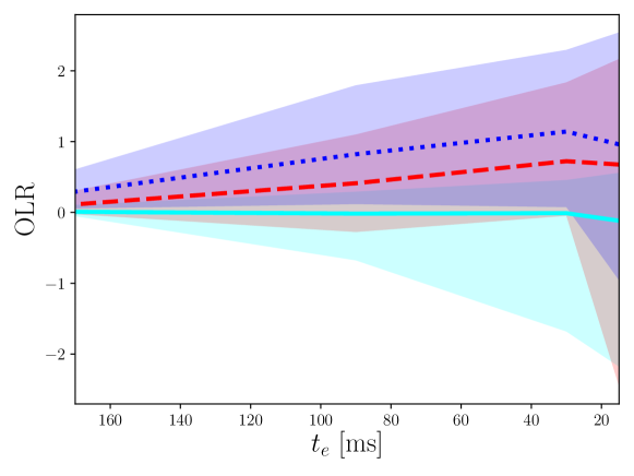
Figure 9: ORL as a function of the gate end-time $t_{e}$ for the exploration set with component masses $(m_{1},m_{2})=(35,29)$ $M_{\odot}$, gate duration $t_{d}=130$ ms, and different network SNR $\rho_{N}=11.3$ (cyan solid), $\rho_{N}=28.3$ (red dashed), and $\rho_{N}=42.4$ (blue dashed). The curves denote median values. Shaded areas are 1-$\sigma$ percentiles.

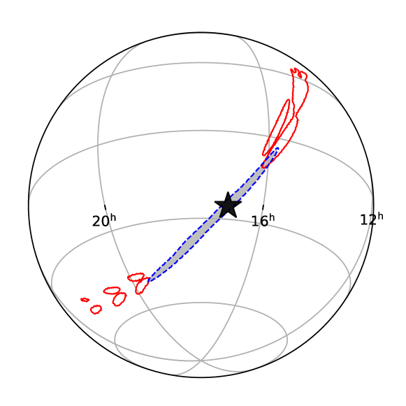
Figure 10: The 90% probability sky localization error regions obtained with the reconstructed (dashed-blue), full (gray area) and gated (solid-red) time series for the case of Fig. 1. The star denotes the injection location.

In summary, for a majority of the cases with gate durations up to a few hundreds of milliseconds and as close as a few tens of milliseconds to the merger time, the sky maps of reconstructed time series with network SNR $\rho_{N}\geq 28.3$ better overlap with the sky maps of the full time series compared to the sky maps obtained with gated data (in some cases by a factor up to over 1000%). In these cases, it can also be shown that the true direction of the signals typically belong to sky localization error regions for the reconstructed data with smaller probability contour values than the regions obtained with gated data.

5 Conclusion

In this paper, we have presented NNETFIX, a new machine learning-based algorithm designed to estimate the portion of a BBH GW signal that may be gated due to the presence of an overlapping glitch. We have tested the accuracy of the algorithm with different choices of signal parameters and gate settings, and defined several metrics to assess NNETFIX’s performance. Among these metrics, the most important ones are the FMG and the ORL.

The FMG quantifies the algorithm’s efficiency in reconstructing the gated data in the time domain. Positive values of this metric indicate that the full time series better matches the NNETFIX reconstructed time series than the gated time series. The fraction of samples that show improvement varies from approximately one third to over 95% across the cases that we investigated. Results show that NNETFIX may be able to successfully reconstruct a majority of BBH signals with peak single interferometer SNR greater than 20 and gates with durations up to a few hundreds of milliseconds as close as a few tens of milliseconds before their merger time.

The ORL quantifies the algorithm’s efficiency in improving the sky map from the gated time series. Positive values of this metric indicate that the sky map from the NNETFIX reconstructed time series has a larger overlap with the sky map from the full time series than the one obtained from the gated data. Sky maps from reconstructed data improve for higher network SNR values as the ANN can use a larger amount of signal energy to estimate the missing portion of the waveform. We find positive ORL median values for all cases that we investigated with network SNR above 28.3. Perhaps surprisingly, NNETFIX seems also to perform better in cases with longer gate durations or shorter signals. In these scenarios, the sky localizations obtained with gated data are considerably degraded. Thus, the improvements in the reconstructed sky maps are more sizeable. Reconstructed sky maps of more massive BBH mergers typically show significant improvements compared to the sky maps obtained with gated data.

In a real case scenario, we envision NNETFIX to be pre-trained on real noise data from the detectors for a sparse set of models, each covering a region of the five-dimensional parameter space spanned by SNR, component masses, gate duration, and gate end-time before geocentric merger time, as was illustrated in Sec. 2 (but with a finer grid). While the optimal value of the network SNR and the best estimates of the signal component masses are unknown to the observer because of the gating, the gated data and/or the data from the second interferometer may provide a rough estimate of these parameters. The estimated values of these parameters and the known gate parameters can then be used to choose the most appropriate pre-trained model in the NNETFIX bank. Typically, the NNETFIX reconstructed time series will produce a higher single interferometer peak SNR than the gated time series. If that is the case, the known FSG can be used to estimate the optimal single interferometer peak SNR of the (unknown) full time series by fitting the expected roughly linear relation between the FRS and the FSG for the given TT set.

The overlap of the sky map from the NNETFIX reconstructed data with the sky map that could be obtained with the full data (if it were not contaminated by a glitch), $O_{r,f}$, can be estimated by looking at the distribution of the ORL for the TT set at hand. The exploration sets that we investigated show that there is a well-defined correlation between the ORL, the FSG and the overlap between the sky maps obtained from the gated data and the NNETFIX reconstructed data, $O_{r,g}$. If this correlation is generally valid, the ORL can be estimated from the observed values of the $O_{r,g}$ and the FSG using a fit calculated from the TT set used to train the selected NNETFIX model. To expedite this process, the samples in each TT set could be clustered according to the distributions of the ORL, the $O_{r,g}$, and the FSG. A classifier could then be trained to estimate the optimal SNR and sky localization error region of the full signal.

Once NNETFIX has been trained, the CPU time required to reconstruct the data is of the order of a few seconds for gate durations up to hundreds of milliseconds. This short turnout makes the algorithm suitable to be used in low-latency. NNETFIX could also be applied to GW signals other than BBH mergers, such as BNS or NSBH mergers. Therefore, it could be beneficial for rapid follow-up of glitch-contaminated, potentially EM-bright candidate detections. In future work, we intend to explore the application of NNETFIX and its effect on the sky localization of BNS signals, as well as detector network configurations with more than two detectors. Improving the sky localizations of potentially EM-bright signals could increase the chances of coincident EM and GW observations and lead to a better understanding of the physical properties of their sources.

References

Network SNR		11.3			28.3			42.4
$t_{d}$ [ms]		50	75	130	50	75	130	50	75	130
$t_{e}$ [ms]	15	0.33/0.54/0.14	0.34/0.55/0.11	0.31/0.66/0.04	0.21/0.76/0.03	0.13/0.85/0.01	0.16/0.84/0.00	0.10/0.88/0.02	0.07/0.93/0.01	0.06/0.94/0.00
	30	0.30/0.46/0.24	0.31/0.46/0.23	0.29/0.63/0.08	0.15/0.78/0.07	0.16/0.80/0.04	0.16/0.84/0.01	0.06/0.88/0.06	0.04/0.93/0.04	0.06/0.94/0.01
	90	0.28/0.39/0.33	0.32/0.36/0.32	0.31/0.52/0.17	0.10/0.69/0.21	0.15/0.71/0.13	0.14/0.82/0.05	0.03/0.80/0.17	0.07/0.84/0.09	0.07/0.92/0.01
	170	0.28/0.40/0.33	0.31/0.40/0.29	0.34/0.38/0.27	0.09/0.68/0.23	0.15/0.71/0.14	0.21/0.67/0.12	0.02/0.84/0.14	0.05/0.83/0.13	0.11/0.83/0.06

Table 2: Fraction of samples with FMG $\leq 0$, $0<\text{\acs{FMG}}\leq 1$ and FMG $>1$ for the exploration sets with component masses $(m_{1},m_{2})=(12,10)M_{\odot}$. Boldface entries denote sets where the fraction of samples with $0<\text{\acs{FMG}}\leq 1$ is larger than 50%.

Network SNR		11.3			28.3			42.4
$t_{d}$ [ms]		50	75	130	50	75	130	50	75	130
$t_{e}$ [ms]	15	0.28/0.52/0.19	0.31/0.55/0.15	0.29/0.64/0.06	0.12/0.78/0.10	0.14/0.83/0.03	0.13/0.87/0.01	0.04/0.89/0.06	0.04/0.94/0.02	0.05/0.95/0.00
	30	0.29/0.34/0.37	0.29/0.49/0.22	0.31/0.59/0.10	0.11/0.68/0.21	0.10/0.82/0.08	0.11/0.88/0.01	0.04/0.75/0.21	0.05/0.91/0.04	0.04/0.95/0.01
	90	0.24/0.42/0.34	0.30/0.38/0.32	0.29/0.39/0.32	0.04/0.76/0.20	0.08/0.72/0.20	0.17/0.69/0.15	0.02/0.79/0.20	0.03/0.79/0.19	0.10/0.80/0.10
	170	0.20/0.42/0.37	0.26/0.42/0.32	0.31/0.32/0.36	0.04/0.69/0.27	0.04/0.72/0.23	0.11/0.69/0.19	0.01/0.78/0.21	0.01/0.80/0.19	0.06/0.79/0.15

Table 3: Fraction of samples with FMG $\leq 0$, $0<\text{\acs{FMG}}\leq 1$ and FMG $>1$ for the exploration sets with component masses $(m_{1},m_{2})=(20,15)M_{\odot}$. Boldface entries denote sets where the fraction of samples with $0<\text{\acs{FMG}}\leq 1$ is larger than 50%.

Network SNR		11.3			28.3			42.4
$t_{d}$ [ms]		50	75	130	50	75	130	50	75	130
$t_{e}$ [ms]	15	0.19/0.50/0.31	0.27/0.53/0.20	0.25/0.44/0.31	0.04/0.76/0.20	0.05/0.84/0.11	0.07/0.76/0.17	0.02/0.80/0.19	0.02/0.90/0.08	0.02/0.81/0.17
	30	0.21/0.35/0.45	0.24/0.34/0.42	0.24/0.44/0.32	0.03/0.60/0.37	0.03/0.56/0.41	0.05/0.76/0.19	0.01/0.62/0.37	0.03/0.66/0.31	0.02/0.86/0.12
	90	0.17/0.47/0.36	0.12/0.31/0.57	0.21/0.32/0.47	0.01/0.75/0.24	0.02/0.42/0.57	0.04/0.51/0.46	0.00/0.79/0.21	0.00/0.38/0.62	0.01/0.59/0.40
	170	0.14/0.42/0.44	0.15/0.40/0.45	0.22/0.45/0.33	0.01/0.63/0.36	0.01/0.64/0.35	0.05/0.75/0.20	0.01/0.67/0.32	0.00/0.65/0.35	0.01/0.88/0.11

Table 4: Fraction of samples with FMG $\leq 0$, $0<\text{\acs{FMG}}\leq 1$ and FMG $>1$ for the exploration sets with component masses $(m_{1},m_{2})=(35,29)M_{\odot}$. Boldface entries denote sets where the fraction of samples with $0<\text{\acs{FMG}}\leq 1$ is larger than 50%.

Network SNR		11.3			28.3			42.4
$t_{d}$ [ms]		50	75	130	50	75	130	50	75	130
$t_{e}$ [ms]	15	${0.52}$	${0.53}$	${0.56}$	${0.62}$	${0.71}$	${0.74}$	${0.76}$	${0.83}$	${0.87}$
	30	${0.56}$	${0.53}$	${0.52}$	${0.68}$	${0.73}$	${0.76}$	${0.81}$	${0.85}$	${0.91}$
	90	${0.55}$	${0.51}$	${0.53}$	${0.69}$	${0.65}$	${0.74}$	${0.78}$	${0.79}$	${0.86}$
	170	${0.61}$	${0.58}$	${0.51}$	${0.72}$	${0.64}$	${0.65}$	${0.79}$	${0.77}$	${0.76}$

Table 5: Fraction of samples with positive ORL for the exploration sets with component masses $(m_{1},m_{2})=(12,10)M_{\odot}$.

Network SNR		11.3			28.3			42.4
$t_{d}$ [ms]		50	75	130	50	75	130	50	75	130
$t_{e}$ [ms]	15	${0.51}$	0.49	${0.55}$	${0.68}$	${0.74}$	${0.79}$	${0.84}$	${0.85}$	${0.84}$
	30	0.46	0.48	${0.51}$	${0.69}$	${0.76}$	${0.80}$	${0.85}$	${0.88}$	${0.88}$
	90	${0.61}$	${0.50}$	0.47	${0.74}$	${0.75}$	${0.65}$	${0.86}$	${0.85}$	${0.79}$
	170	${0.62}$	${0.56}$	0.47	${0.77}$	${0.78}$	${0.67}$	${0.84}$	${0.87}$	${0.82}$

Table 6: Fraction of samples with positive ORL for the exploration sets with component masses $(m_{1},m_{2})=(20,15)M_{\odot}$. Entries in italic denote sets where the fraction of samples is smaller than 0.5.

Network SNR		11.3			28.3			42.4
$t_{d}$ [ms]		50	75	130	50	75	130	50	75	130
$t_{e}$ [ms]	15	${0.57}$	${0.53}$	0.43	${0.77}$	${0.79}$	${0.69}$	${0.85}$	${0.83}$	${0.73}$
	30	${0.51}$	0.45	0.49	${0.81}$	${0.81}$	${0.82}$	${0.91}$	${0.87}$	${0.87}$
	90	${0.65}$	${0.63}$	0.46	${0.84}$	${0.80}$	${0.75}$	${0.93}$	${0.89}$	${0.87}$
	170	${0.65}$	${0.64}$	${0.57}$	${0.79}$	${0.84}$	${0.80}$	${0.88}$	${0.91}$	${0.91}$

Table 7: Fraction of samples with positive ORL for the exploration sets with component masses $(m_{1},m_{2})=(35,29)M_{\odot}$. Entries in italic denote sets where the fraction of samples is smaller than 0.5.

Network SNR		11.3			28.3			42.4
$t_{d}$ [ms]		50	75	130	50	75	130	50	75	130
$t_{e}$ [ms]	15	${0.0012}$	${0.0064}$	${0.0096}$	${0.016}$	${0.031}$	${0.056}$	${0.051}$	${0.086}$	${0.14}$
	30	${0.0044}$	${0.0059}$	${0.0022}$	${0.015}$	${0.028}$	${0.044}$	${0.044}$	${0.073}$	${0.14}$
	90	${0.0032}$	${0.0005}$	${0.0021}$	${0.0091}$	${0.011}$	${0.034}$	${0.026}$	${0.04}$	${0.10}$
	170	${0.0026}$	${0.0037}$	${0.0007}$	${0.0076}$	${0.0063}$	${0.018}$	${0.018}$	${0.032}$	${0.060}$

Table 8: Median values of ORL for the exploration sets with component masses $(m_{1},m_{2})=(12,10)M_{\odot}$.

Network SNR		11.3			28.3			42.4
$t_{d}$ [ms]		50	75	130	50	75	130	50	75	130
$t_{e}$ [ms]	15	${0.0023}$	-0.0007	${0.016}$	${0.054}$	${0.087}$	${0.17}$	${0.16}$	${0.24}$	${0.32}$
	30	-0.0050	-0.0029	${0.0039}$	${0.044}$	${0.079}$	${0.15}$	${0.13}$	${0.22}$	${0.31}$
	90	${0.0049}$	${0.0002}$	-0.0051	${0.025}$	${0.046}$	${0.050}$	${0.074}$	${0.13}$	${0.25}$
	170	${0.0047}$	${0.0051}$	-0.0044	${0.023}$	${0.037}$	${0.045}$	${0.046}$	${0.098}$	${0.17}$

Table 9: Median values of ORL for the exploration sets with component masses $(m_{1},m_{2})=(20,15)M_{\odot}$. Italic entries denote sets with negative values.

Network SNR		11.3			28.3			42.4
$t_{d}$ [ms]		50	75	130	50	75	130	50	75	130
$t_{e}$ [ms]	15	${0.023}$	${0.0098}$	-0.1400	${0.33}$	${0.45}$	${0.68}$	${0.62}$	${0.82}$	${0.96}$
	30	${0.0032}$	-0.043	-0.0099	${0.25}$	${0.42}$	${0.72}$	${0.56}$	${0.83}$	${1.1}$
	90	${0.013}$	${0.024}$	-0.015	${0.088}$	${0.21}$	${0.41}$	${0.24}$	${0.48}$	${0.82}$
	170	${0.012}$	${0.016}$	${0.0085}$	${0.046}$	${0.081}$	${0.11}$	${0.12}$	${0.22}$	${0.29}$

Table 10: Median values of ORL for the exploration sets with component masses $(m_{1},m_{2})=(35,29)M_{\odot}$. Italic entries denote sets with negative values.

References

- [1] Abbott B P et al. (Virgo, LIGO Scientific) 2016 Phys. Rev. Lett. 116 061102 (Preprint 1602.03837)
- [2] Aasi J et al. (LIGO Scientific) 2015 Class. Quant. Grav. 32 074001 (Preprint 1411.4547) URL http://stacks.iop.org/0264-9381/32/i=7/a=074001
- [3] Acernese F et al. (VIRGO) 2015 Class. Quant. Grav. 32 024001 (Preprint 1408.3978) URL http://stacks.iop.org/0264-9381/32/i=2/a=024001
- [4] Abbott B P et al. (LIGO Scientific Collaboration and Virgo Collaboration) 2019 Phys. Rev. X 9(3) 031040 URL https://link.aps.org/doi/10.1103/PhysRevX.9.031040
- [5] Abbott R et al. (LIGO Scientific, Virgo) 2020 (Preprint 2010.14527)
- [6] Abbott R et al. (LIGO Scientific, Virgo) 2020 Phys. Rev. D 102 043015 (Preprint 2004.08342)
- [7] Abbott R et al. (LIGO Scientific Collaboration and Virgo Collaboration) 2020 Phys. Rev. Lett. 125(10) 101102 URL https://link.aps.org/doi/10.1103/PhysRevLett.125.101102
- [8] Abbott R et al. 2020 The Astrophysical Journal 900 L13 URL https://doi.org/10.3847%2F2041-8213%2Faba493
- [9] Abbott R et al. (LIGO Scientific, Virgo) 2020 Astrophys. J. 896 L44 (Preprint 2006.12611)
- [10] Abbott B P et al. (LIGO Scientific Collaboration and Virgo Collaboration) 2017 Phys. Rev. Lett. 119(16) 161101 URL https://link.aps.org/doi/10.1103/PhysRevLett.119.161101
- [11] Abbott B P et al. (GROND, SALT Group, OzGrav, DFN, INTEGRAL, Virgo, Insight-Hxmt, MAXI Team, Fermi-LAT, J-GEM, RATIR, IceCube, CAASTRO, LWA, ePESSTO, GRAWITA, RIMAS, SKA South Africa/MeerKAT, H.E.S.S., 1M2H Team, IKI-GW Follow-up, Fermi GBM, Pi of Sky, DWF (Deeper Wider Faster Program), Dark Energy Survey, MASTER, AstroSat Cadmium Zinc Telluride Imager Team, Swift, Pierre Auger, ASKAP, VINROUGE, JAGWAR, Chandra Team at McGill University, TTU-NRAO, GROWTH, AGILE Team, MWA, ATCA, AST3, TOROS, Pan-STARRS, NuSTAR, ATLAS Telescopes, BOOTES, CaltechNRAO, LIGO Scientific, High Time Resolution Universe Survey, Nordic Optical Telescope, Las Cumbres Observatory Group, TZAC Consortium, LOFAR, IPN, DLT40, Texas Tech University, HAWC, ANTARES, KU, Dark Energy Camera GW-EM, CALET, Euro VLBI Team, ALMA) 2017 Astrophys. J. 848 L 12 (Preprint 1710.05833)
- [12] Abbott B P et al. (Virgo, Fermi-GBM, INTEGRAL, LIGO Scientific) 2017 Astrophys. J. 848 L13 (Preprint 1710.05834)
- [13] Abbott B et al. (LIGO Scientific, Virgo) 2020 Astrophys. J. Lett. 892 L3 (Preprint 2001.01761)
- [14] Driggers J et al. (LIGO Scientific) 2019 Phys. Rev. D 99 042001 (Preprint 1806.00532)
- [15] Usman S A et al. 2016 Class. Quant. Grav. 33 215004 (Preprint 1508.02357)
- [16] Pankow C et al. 2018 Phys. Rev. D 98(8) 084016 URL https://link.aps.org/doi/10.1103/PhysRevD.98.084016
- [17] Cornish N J and Littenberg T B 2015 Classical and Quantum Gravity 32(13) 135012 URL https://doi.org/10.1088/0264-9381/32/13/135012
- [18] Pedregosa F, Varoquaux G, Gramfort A, Michel V, Thirion B, Grisel O, Blondel M, Prettenhofer P, Weiss R, Dubourg V, Vanderplas J, Passos A, Cournapeau D, Brucher M, Perrot M and Duchesnay E 2011 Journal of Machine Learning Research 12 2825–2830
- [19] Rosenblatt F 1961 Principles of neurodynamics. perceptrons and the theory of brain mechanisms Tech. rep. Cornell Aeronautical Lab Inc Buffalo NY
- [20] Nair V and Hinton G E 2010
- [21] Kingma D and Ba J 2014 International Conference on Learning Representations
- [22] Khan S, Husa S, Hannam M, Ohme F, Pürrer M, Forteza X J and Bohé A 2016 Phys. Rev. D 93(4) 044007 URL https://link.aps.org/doi/10.1103/PhysRevD.93.044007
- [23] Cokelaer T 2007 Phys. Rev. D 76 102004 (Preprint 0706.4437)
- [24] Harry I W, Allen B and Sathyaprakash B 2009 Phys. Rev. D 80 104014 (Preprint 0908.2090)
- [25] Van Den Broeck C, Brown D A, Cokelaer T, Harry I, Jones G, Sathyaprakash B, Tagoshi H and Takahashi H 2009 Phys. Rev. D 80 024009 (Preprint 0904.1715)
- [26] Manca G M and Vallisneri M 2010 Phys. Rev. D 81 024004 (Preprint 0909.0563)
- [27] Chatterji S, Blackburn L, Martin G and Katsavounidis E 2004 Class. Quant. Grav. 21 S1809–S1818 (Preprint gr-qc/0412119)
- [28] Nitz A, Harry I, Brown D, Biwer C M, Willis J, Canton T D, Capano C, Pekowsky L, Dent T, Williamson A R, Davies G S, De S, Cabero M, Machenschalk B, Kumar P, Reyes S, Macleod D, Pannarale F, dfinstad, Massinger T, Tápai M, Singer L, Khan S, Fairhurst S, Kumar S, Nielsen A, shasvath, Dorrington I, Lenon A and Gabbard H 2020 gwastro/pycbc: Pycbc release 1.16.4 URL https://doi.org/10.5281/zenodo.3904502
- [29] Ashton G, Burns E, Canton T D, Dent T, Eggenstein H B, Nielsen A B, Prix R, Was M and Zhu S J 2018 The Astrophysical Journal 860 6 URL https://doi.org/10.3847%2F1538-4357%2Faabfd2