Gravitational waves from inspiralling compact binaries: hexagonal template placement and its efficiency in detecting physical signals.

Abstract

Matched filtering is used to search for gravitational waves emitted by inspiralling compact binaries in data from the ground-based interferometers. One of the key aspects of the detection process is the design of a template bank that covers the astrophysically pertinent parameter space. In an earlier paper, we described a template bank that is based on a square lattice. Although robust, we showed that the square placement is over-efficient, with the implication that it is computationally more demanding than required. In this paper, we present a template bank based on an hexagonal lattice, which size is reduced by 40% with respect to the proposed square placement. We describe the practical aspects of the hexagonal template bank implementation, its size, and computational cost. We have also performed exhaustive simulations to characterize its efficiency and safeness. We show that the bank is adequate to search for a wide variety of binary systems (primordial black holes, neutron stars and stellar mass black holes) and in data from both current detectors (initial LIGO, Virgo and GEO600) as well as future detectors (advanced LIGO and EGO). Remarkably, although our template bank placement uses a metric arising from a particular template family, namely stationary phase approximation, we show that it can be used successfully with other template families (e.g., Padé resummation and effective one-body approximation). This quality of being effective for different template families makes the proposed bank suitable for a search that would use several of them in parallel (e.g., in a binary black hole search). The hexagonal template bank described in this paper is currently used to search for non-spinning inspiralling compact binaries in data from the Laser Interferometer Gravitational-Wave Observatory (LIGO).

I Introduction

Ground-based laser interferometer detectors such as Laser Interferometer Gravitational wave Observatory (LIGO) [1] or Virgo [2] are expected to detect gravitational wave (GW)-signals in data that have been, or will soon be, collected. The most promising and well-understood astrophysical sources of gravitational waves are inspiralling compact binaries (ICB) in close orbits [3], which consist of two compact objects such as primordial black holes, neutron stars and/or stellar-mass black holes.

Potentiality of a detection verges towards one event per year. However, the detection rate strongly depends on the ICB coalescence rate  [5, 4, 6] and the volume of universe that detectors can probe. While we cannot influence the coalescence rates, we can increase the volume or distance at which a signal can be detected, which highly depends on (i) the design of the detectors and their sensitivities, and (ii) on the detection technique that is used. Detector sensitivity can be increased most certainly; but once data have been recorded, only the deployment of an optimal method of detection can ensure the highest detection probability, and that is a passport, not only to probe the largest volume of Universe possible, but also to detect a GW-signal directly for the first time. Fortunately enough, altough the two body problem cannot be solved exactly in general relativity, post-Newtonian (hereafter PN) approximation have been used to obtain accurate models of the late-time dynamics of ICB [7]. Therefore, we can deploy a matched filtering technique, which is an optimal method of detection when the signal buried in Gaussian and stationary noise is known exactly. The models that we used for detection are also called template families.

The shape of the incoming GW-signals depends on various parameters, which are not known a priori (e.g., the masses of the two component stars in the case of a search for non-spinning binaries). Thus, we have no choice but to filter the data through a set of templates, which is also called a template bank and must cover the parameter space that is astrophysically relevant. Since we cannot filter the data through an infinitely large number of templates the bank is essentially discrete. Consequently, the mismatch between any signal and the nearest template in the discrete template bank will cause reduction in the signal-to-noise ratio (SNR). Spacing between templates must be chosen so as to render acceptable this SNR reduction as well as the computational demand required by the cross correlation of the data with the entire discrete template bank. As we shall see, the spacing between templates is set by specifying a minimal match between any signal and the template bank. In practice, template families are approximation of the true gravitational wave signal, and no true signal will perfectly match any of the template families. However, in this paper we shall consider that template and simulated signal belong to the same template family.

The template bank placement is one of the key aspects of the detection process. Nonetheless, its design is not unique. There are essentially two types of template bank placements. The first one does not assume any knowledge on the signal manifold; the second does. The first type of placement computes matches between surrounding templates until two templates have a match close to the requested minimal match, and computes matches repeatedly over the entire parameter space until it is fully populated. Using geometrical considerations, an efficient instance of this technique has been developed [9]. A second approach, described in various papers [10, 11, 12], utilizes a metric that is defined on the signal manifold. It uses local flatness theorem to place templates at proper distances [10] over the parameter space. We developed a template bank placement in [12] that was implemented and fully tested within the LIGO algorithm library [14]. This template bank was used in the analysis of data from different LIGO science runs  [15, 16, 17, 18, 19]. We also shown that although robust with respect to the requirement (matches should be above the minimal match), it is over-efficient. This result was expected because we used a square lattice to place templates over the parameter space.

In this paper, we fully describe and validate a hexagonal template bank placement that is currently used by the LIGO scientific collaboration so as to analyze the most recent science runs. In Section II, we recapitulate some fundamental techniques and notions that are needed to describe the bank placement, and previous results on the square template bank placement. We also provide a framework to validate a template bank. In Section III, we describe the algorithm that places templates on a hexagonal lattice. In Section IV, we summarize the outcome of the simulations performed to test the hexagonal bank. We envisage various parameter spaces that allows to search for binary neutron star (BNS), primordial black hole (PBH), black hole - neutron star (BHNS) and, or binary black hole (BBH) signals. We also considered design sensitivity curves for the current and advanced generation of ground-based detectors. In Section IV.2, we show that the proposed hexagonal template bank has the required specifications.

Finally, in addition to the case of a template family based on the stationary phase approximation, we also investigate in Section IV.3 the possibility to use the same hexagonal bank placement with other template families including Padé resummation and effective one-body approximation. We show that there is no need to construct specific template bank for each template family: the proposed bank can be used for the different families that we looked at in this paper.

II Formalism and template bank validation

Matched filtering and template bank placement use formalisms that are summarized in this Section. We also review the main results of the square placement, and recapitulate the framework introduced in [12] that allows us to validate a template bank.

II.1 Signal and Metric

The matched filtering technique is an optimal method to detect a known signal, $s(t)$, that is buried in a stationary and Gaussian noise, $n(t)$ [20]. The method performs a correlation of the data $x(t)=n(t)+s(t)$ with a template $h(t)$. In this paper, we shall assume that $s(t)$ and $h(t)$ are generated with the same model so that a template can be an exact copy of the signal. Matched filtering of the data $x(t)$ with a template $h(t)$ can be expressed via the inner product weighted by the noise power spectral sensitivity (PSD), $S_{h}(f)$, and is given by

$$(x,h)=2\int_{0}^{\infty}\frac{\tilde{x}^{*}(f)\tilde{h}(f)+\tilde{x}(f)\tilde{h}^{*}(f)}{S_{h}(f)}df\,.$$ (1)

Note that for simplicity, we will ignore the time $t$ within the inner product expressions. A template and a signal can be normalized according to

$$\hat{h}=\frac{h}{\sqrt{(h,h)}},\,\hat{s}=\frac{s}{\sqrt{(s,s)}}\,.$$ (2)

The SNR after filtering by $h(t)$ is

$$\rho=\frac{(x,h)}{\sqrt{(h,h)}}=(x,\hat{h}).$$ (3)

The simulations that we will perform assume that template and signal are normalized, that is $(\hat{h},\hat{h})=1$, and $(\hat{s},\hat{s})=1$. In this paper, we are interested in the fraction of the optimal SNR obtained by filtering the signal $x(t)$ with a set of template $h(t)$, therefore, we can ignore the noise $n(t)$, and $(x,\hat{h})$ becomes $(\hat{s},\hat{h})$. Strictly speaking, $(\hat{s},\hat{h})$ does not refer to a SNR anymore, but to the ambiguity function, which is by definition always less than or equal to unity if the two waveforms are normalized. In the following, we shall use the notion of match introduced in [10]; the match between two templates is the inner product between two templates that is maximized over the time (using the inverse Fourier transform) and the initial orbital phase (using a quadrature matched filtering).

The incoming signal has unknown parameters and one needs to filter the data through a set of templates, i.e., a template bank. The templates are characterized by a set of $p$ parameters $\vartheta^{\mu},\;\mu=0,1,..,p-1$. The templates in the bank are copies of the signal corresponding to a set of values $\vartheta^{\mu}_{i},\;i=0,1,..,N_{b}-1$, where $N_{b}$ is the total number of templates. A template bank is optimally designed if $N_{b}$ is minimal and if for any signal there always exists at least one template in the bank such that

$$\min_{\vartheta^{{}^{\prime}\mu}}\max_{i}(\hat{s}(\vartheta^{{}^{\prime}\mu}),\hat{h}(\vartheta^{\mu}_{i}))\geq MM,$$ (4)

where $MM$ is the minimal match mentioned earlier. Usually, in searches for ICB, the value of the minimal match is set by the user to 95% or 97%, which corresponds to a decrease in detection rate of 15% and 9%, respectively. Nevertheless, the minimal match may have a much smaller value for the first stage of a hierarchical search (e.g., 80%), or for a one-stage search of periodic signals (e.g., 70% or lower).

The distance between two infinitesimally separated normalized templates on the signal manifold is given by [10, 11]

$$||h(\vartheta^{\mu}+d\vartheta^{\mu})-h(\vartheta^{\mu})||^{2} = \left|\left|h_{\mu}d\vartheta^{\mu}\right|\right|^{2}$$ (5)

$$= \left(h_{\mu},h_{\nu}\right)\,d\vartheta^{\mu}d\vartheta^{\nu}$$

$$\equiv g_{\mu\nu}d\vartheta^{\mu}d\vartheta^{\nu},$$

where $h_{\mu}$ is the partial derivative of the signal $h$ with respect to the parameter $\vartheta^{\mu}$. So, the quadratic form

$$g_{\mu\nu}=(h_{\mu},h_{\nu})$$ (6)

defines the $g_{\mu\nu}$ metric induced on the signal manifold. The metric is used to place templates at equal distance in the parameter space. The distance $dx_{i}$ between templates in each dimension is given by

$$dx_{i}=2\sqrt{\frac{1-MM}{g_{ii}}},i=0,1,..,p-1\,.$$ (7)

In practice, using such $dx_{i}$ leaves a fraction of the parameter space uncovered, and overlap between templates is required (e.g., in the square placement, spacing is actually set to $dx_{i}/\sqrt{2}$).

Since we restrict ourself to the case of non-spinning waveforms, $h(t)$ depends on 4 parameters only: the two component masses, $m_{1}$ and $m_{2}$ which may vary from sub-solar mass to tens of solar mass systems, the initial orbital phase $\varphi_{C}$, and the time of coalescence $t_{C}$. We can maximized over $t_{C}$ and $\varphi_{C}$ analytically, therefore the parameter space that we need to cover with our template bank is a 2-dimensional space only. For conciseness, we can represent the GW-waveform with a simplified expression given by

$$h(t)=\frac{4A\eta M}{D}\left[\pi Mf(t)\right]^{2/3}\cos[\varphi(t)+\varphi_{C}],$$ (8)

where $f(t)$ is the (invariant) instantaneous frequency of the signal measured by a remote observer, the phase of the signal $\varphi(t)=2\pi\int^{t_{C}}f(t)dt$ is defined so that it is zero when the binary coalesces at time $t=t_{C}$, and $A$ is a numerical constant representing the amplitude [21]. The asymmetric mass ratio is $\eta=m_{1}m_{2}/M^{2}$, where $M=m_{1}+m_{2}$ is the total mass of the system. There exist amplitude corrections up to 2.5PN [8], the importance of which for detection and estimation is shown in [22]. However, in this work, we use restricted post-Newtonian models only and limit PN-expansion of the phase to 2PN order. Moreover, in the template bank placement, namely for the metric computation, we consider the stationary phase approximation (SPA) [23], for which the metric can be derived analytically [12]. Nevertheless, other template families can be used both for injection and filtering (see Section IV.1).

II.2 Example : the Square Template Bank

The placement that we proposed in [12] uses the metric based on the SPA model, and the spacing $dx_{i}$, as defined in Eq. (7). Since the model $h$ explicitly depends on the two mass parameters $M$ and $\eta$, then the spacing $dx_{i}$ are function of these two quantities as well. However, the metric expressed in these two coordinates is not a constant; it is not a constant either if we were to use the component masses, $m_{1}$ and $m_{2}$. The preference of chirptimes, denoted $\tau_{0}$ and $\tau_{3}$ (see appendix B, Eqs. 18) as coordinates on the signal manifold is indeed more practical because these variables are almost Cartesian [24, 23]. Although not perfectly constant for PN-order larger than 1PN, we shall assume that the metric is essentially constant in the local vicinity of every point on the manifold. We could use any combinations of chirptimes, but using the pair $\tau_{0}-\tau_{3}$, there exists analytical inversion with the pair $M-\eta$ (see appendix 19).

The parameter space to be covered is defined by the minimum and maximum component masses of the systems considered ($m_{\rm min}$ and $m_{\rm max}$), and possibly the minimum and maximum total mass ($M_{\rm min}$ and $M_{\rm max}$) as shown in Fig. 1. The lower cut-off frequency $f_{L}$, at which the template starts in frequency, sets the length of the templates and therefore directly influences the metric components, the parameter space, and the number of templates $N_{b}$. In [12], we showed how the size of the template bank changes with $f_{L}$. We also investigated the loss of match due to the choice of $f_{L}$. We generally set $f_{L}$ so that the loss of match is of the order of a percent.

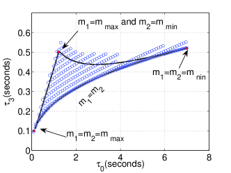
Figure 1: Example of parameter space and template bank placement. The parameter space is defined by the individual mass components (from $3~{}M_{\odot}$ to $30~{}M_{\odot}$) and the lower cut-off frequency ($f_{L}=40$ Hz). The bottom line corresponds to $m_{1}=m_{2}$, or equivalently to $\eta=0.25$. The two other boundaries meet where $m_{1}=m_{\rm min}$ and $m_{2}=m_{\rm max}$. The bottom left point of the parameter space corresponds to $m_{1}=m_{2}=m_{\rm max}$ whereas the top right point corresponds to $m_{1}=m_{2}=m_{\rm min}$. The gray/blue circles give the position of each template that is needed to cover the entire parameter space (black curves). Even though some templates lie outside the parameter space boundaries, these are required to fully cover the parameter space.

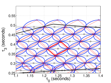
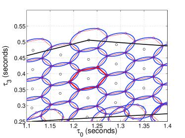
Figure 2: Two instances of template bank placements. In the two plots, we focus on a small area of the parameter space presented in figure 1. We used a square (top panel) and hexagonal (bottom panel) placement. For convenience, we re-scale the metric components so that, $g_{00}\sim g_{11}$. Each template position is represented by a small circle. Around each template position, we plot an ellipse that represents iso-match contour of $MM=0.95\%$. Each ellipse contains an inscribed square or hexagon which emphasizes how ellipses overlap each other. We can see that squares (top) slightly overlap each other. This is because templates are layed along $\tau_{3}$ equal constant line and not along the eigen-vector directions, which change over the parameter space. In the hexagonal placement, we take care of this problem short-coming, and therefore hexagons are perfectly adjacent to each other: the placement is optimal.

We briefly remind how the proposed square template bank works. First, templates are placed along the $m_{1}=m_{2}$ or $\eta=0.25$ line starting from the minimum to the maximum mass. Then, additional templates are placed so as to cover the remaining part of the parameter space, in rows, starting at $\eta=0.25$ along lines of constant $\tau_{3}$ until a template lies outside the parameter space. The spacing between lines is set adequately. Distances between templates are based on a square lattice. An example of such a placement is shown in Fig. 2. One of the limitations of the placement is that templates are not placed along the eigenvectors of the metric but along the standard basis vectors that describe the $\tau_{0},\tau_{3}$ space. This approximation make the ellipses slightly more overlapping than requested and may also create holes when the orientation of the ellipses varies significantly (i.e., at high mass regime). The square placement is also over-efficient as compared to a hexagonal placement (see Fig. 3).

II.3 Bank Efficiencies

Independently of the template bank placement, the template bank must be validated to check whether it fulfills the requirements (e.g., from Eq. 4). First, we perform Monte-Carlo simulations so as to compute the efficiency vector, $\mathcal{E}$, given by

$$\mathcal{E}\left(\mathcal{\chi}_{s},\mathcal{\chi}_{h}\right)=\left\{\max_{j}\left(\hat{s}(\vartheta^{s}_{i}),\hat{h}(\vartheta^{h}_{j})\right)\right\}_{i=1..N_{s},j=1..N_{b}}$$ (9)

where $N_{b}$ is the number of templates in the bank, $N_{s}$ the number of injections.

The vectors $\vartheta^{s}$ and $\vartheta^{h}$ correspond to the parameters of the simulated signals and the templates, $\chi_{s}$ and $\chi_{h}$ are the models used in the generation of the signal and template, respectively. In all the simulations, we set $\vartheta^{s}=\{m_{1},m_{2},\varphi_{C},t_{C}\}$. Furthermore, we can analytically maximize over the unknown orbital phase $\varphi_{C}$ and, therefore, $\vartheta^{h}=\{m_{1},m_{2}\}$.

The efficiency vector $\mathcal{E}$ and the signal parameter vector $\vartheta^{s}$ are useful to derive several figures of merit. The cumulative distribution of $\mathcal{E}$ (Fig. 3, bottom panel) indicates how quickly matches drop as the minimal match is reached. Nevertheless, the cumulative distribution function of $\mathcal{E}$ hides the dependency of the matches upon masses. Therefore, we also need to look at the distribution of $\mathcal{E}$ versus total mass $M$ (e.g., Fig. 3, top panel), or versus $\eta$, or chirp mass, $\mathcal{M}$ (see appendix for an exact definition). Usually, we look at $\mathcal{E}_{M}$ only. Indeed, in most cases, the dynamical range of $\eta$ is small (from 0.1875 to 0.25 in the BNS case). Finally, we can quantify the efficiency of a template bank with a unique value, that is the safeness, $\mathcal{S}$, given by

$$\mathcal{S}_{\mathcal{R}}\left(\mathcal{\chi}_{s},\mathcal{\chi}_{h}\right)=\min\mathcal{E}(\chi_{s},\chi_{h}).$$ (10)

Ideally, we should have a template bank such that $\mathcal{S}_{\mathcal{R}}\approx MM$. $\mathcal{S}_{\mathcal{R}}$ is a generalization of the left hand side of Eq. 4 on $N_{s}$ injections. The higher $N_{s}$ is, the more confident we are with the value of the safeness. Ideally, the number $N_{s}$ should be several times the size of the template bank that is $N_{s}\gg N_{b}$, so that statistically we have at least one injection per template. The sub-index $\mathcal{R}$ of the safeness is the ratio between $N_{s}$ and $N_{b}$ and indicates the relevance of the simulations. The safeness provides also a way of characterizing the template bank: if $\mathcal{S}_{\mathcal{R}}$ is less than the expected minimal match $MM$, then the bank is under-efficient. Conversely, a template bank can be over-efficient like in Fig. 3.

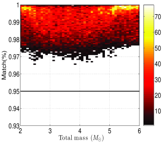
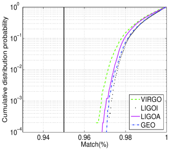
Figure 3: Efficiencies of the square template bank. For convenience we remind the reader of some results of the square template bank provided in  [12]. In the simulations, we used stationary phase approximant models for both injections and templates. Injections consist of binary neutron stars. We used 4 design sensitivity curves (LIGOI, advanced LIGO, VIRGO and GEO), and for each of them we performed 10,000 injections. In the top panel, we show all the results together: all injections are recovered with a match higher than 95%, as requested. In the bottom panel, we decomposed the 4 simulations and show that all of them behave similarly. Actually, we can see that most of the injections are recovered with even higher matches (above 97%) showing the over-efficiency of the placement.

III Hexagonal placement based on the metric

In the $\tau_{0},\tau_{3}$ basis vectors, both amplitude and orientation of the eigenvectors change, which may imply a laborious placement. In this Section, we describe the hexagonal placement that is conceptually different from the square placement and takes into account the eigenvectors change throughout the parameter space.

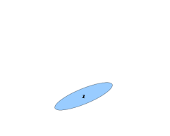
(a) Initialization

(b) Reproduction cell 1

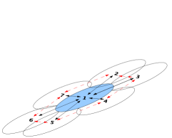
(c) Connections

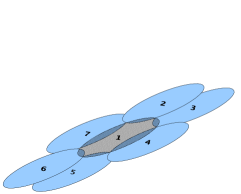
(d) Initialization

(e) Reproduction cell 2

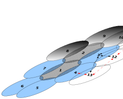
(f) Reproduction cell 3

Figure 4: Hexagonal template bank placement. Using the terminology that is introduced in the text, we can describe the template bank placement algorithm as follows. First, in sub-figure (a), a cell/template is arbitrary placed in the parameter space. Its coordinates correspond to $m_{1}=m_{\rm min}$ and $m_{2}=m_{\rm max}$, and its Id is 1. In sub-figure (b), the cell with ID=1, which is also a mother cell, reproduces 6 new cells according to an optimal hexagonal lattice that takes into account its metric components. In sub-figure (c) the connection between the offsprings and the mother cell are created (black arrows). Cells that belong to the same generation (white ellipses) are also connected if there are adjacent to each other (red arrows). In sub-figure (d), the new cells can start to reproduce. However, the reproduction is exclusive: reproduction takes place cell after cell, and the cell with lowest ID is chosen to reproduce first. In sub-figure (e), therefore, the cell with ID equals 2 starts to reproduce. Because connections already exist with other cells, this cell will reproduce only 3 directions (i.e., 8, 9 and 10). In sub-figure (f), the cell with ID equals 3 starts to populate. The 3 new cells (gray ellipses) created by the cell with ID=2 have to wait for the current generation (blue ellipse) to fully reproduce. The cells spread until the boundary of the parameter space is reached.

III.1 Algorithm

Although the hexagonal placement algorithm is independent of any genetic or evolutionary algorithms, it can be compared to biological process, and we will use this analogy to explain the placement. First, let us introduce a cell that contain a template position (e.g., $\tau_{0}-\tau_{3}$), the metric components defined at this position, and a unique identification number that we refer to as an ID. A cell covers an area defined by an ellipse with semi-axis equal to $dx_{i}/2$. The goal of a cell is to populate the parameter space with an offspring of at most 6 cells (hexagonal placement). A cell can be characterized by the following principles:

1-Initialization

A cell is created at a given position in $\tau_{0}-\tau_{3}$ plane, not necessarily at a physical place (i.e, $\eta$ can be less than 1/4). The initialization requires that

• metric components at $(\tau_{0}-\tau_{3})$ are calculated,

• a unique ID number is assigned,

• 6 connectors are created and set to zero.

Finally, if the cell area intersects with the parameter space, then it has the ability to survive in its environment: it is fertile. Conversely, a cell whose coverage is entirely outside the parameter space is sterile.

2-Reproduction

A fertile cell can reproduce into 6 positions that are the corner of a hexagon inscribed in the ellipse whose semi-axes are derived from the metric components $dx_{i}$’s. A cell that has reproduced is a mother cell and its offspring is composed of 6 daughter cells. Once a daughter cell is initialized, it cannot reproduce in place of its mother. This is taken into account via the connection principle.

3-Connection

Following the reproduction process, a mother cell sets the connections with its daughter cells by sharing their IDs. Therefore, a mother cell knows the IDs of its daughter cells and vice-versa. Moreover, when a mother cell reproduces, it also sets up the connections between two adjacent daughters so that they both know their IDs. These connections prevent cells to reproduce in a direction that is already populated.

4-Sterility

A cell becomes sterile (cannot reproduce anymore) when both reproduction and connection principles have been applied. A cell that is outside the parameter space is also sterile (checked during the initialization).

5-Exclusivity

The reproduction process is exclusive: only one cell at a time can reproduce. It is exclusive because a cell cannot start to reproduce while another cell is still reproducing.

The cell population evolves by the reproduction of their individuals over as many generations as needed to cover the entire parameter space. The first generation is composed of one cell only. The position of this first cell corresponds to $m_{1}=m_{\rm min},m_{2}=m_{\rm max}$. We could start at any place in the parameter space. However, local flatness is an approximation and the author thinks it is better NOT to start at $m_{1}=m_{\rm max},m_{2}=m_{\rm max}$ where the metric evolves quicker (highest mass). The first cell is initialized (first principle). Then, the cell reproduces into 6 directions (second principle). Once the reproduction is over, the connectors between the mother cell and its daughters are set (third principle), and finally, the cell becomes sterile (fourth principle). This loop over the first cell has created a new generation of 6 cells, and each cell will now follow the four principles again. However, the new generation of cells will not be able to reproduce in 6 directions. Indeed, connectors between the first mother cell and its daughters have been set, and therefore the new cell generation cannot propagate towards the mother direction. Furthermore, the 6 new cells have already 2 other adjacent cells. Therefore, each cell of the second generation can reproduce 3 times only. Moreover, some of the cells might be outside the parameter space and are sterile by definition. Once a new generation has been created, the previous generation must contain sterile cells only. The algorithm loops over the new generation while there exists fertile cells. The first generation is a particular case since it contains only one cell. However, the following generations are not necessarily made of a unique cell, and the reproduction warrants a careful procedure: the reproduction takes place cell after cell starting from the smallest ID. Moreover, in agreement with the fifth principle, the cells of the newest generation wait until all the cells of the previous generation have reproduced. The reproduction over generations stops once no more fertile cells are present within the population. Since the parameter space is finite, the reproduction will automatically stop. Figure 4 illustrates how the first 3 generations populate the parameter space.

Once the reproduction is over, some cells might be outside the physical parameter space, or outside the mass range requested. An optional final step consists in“pushing back” the corresponding cells inside the parameter space. First, we can push back the non-physical cells only, that is the cells that are below the $\eta=1/4$ line towards the relevant eigen-vector directions onto the $\eta=1/4$ line. Second, there are other cells for which mass parameters correspond to physical masses but that are outside the parameter space of interest. Nothing prevents us from pushing these cells back into the parameter space as well. This procedure is especially important in regions where the masses of the component objects are large. Indeed, keeping templates of mass larger than a certain value causes problems owing to the fact that the search pipeline uses a fixed lower cut-off frequency and the waveforms of mass greater than this value cannot be generated. In the simulations presented in this paper, we move the cells that are below the $\eta=1/4$ boundary, and keep the cells that are outside the parameter space but with $\eta>1/4$. Useful equations that characterize the boundaries of the parameter space are provided in appendix B. A flow chart of the algorithm is also presented in appendix C.

An example of the proposed hexagonal placement is shown in Fig. 1. In this example, the minimum and maximum individual mass component are $3~{}M_{\odot}$ and $30~{}M_{\odot}$, and the lower cut-off frequency is of $40$ Hz. We can see that none of the templates are placed below the equal mass line whereas some are placed outside the parameter space. Figure 2 gives another placement example.

III.2 Size, Gain and Computational Cost

The ratio of a circle’s surface to the area of a square inscribed within this circle is $\pi R^{2}/(2R^{2})\approx 1.57$, where $R$ is the circle’s radius. The ratio of the same circle’s surface to an inscribed hexagon equals $\pi R^{2}/(3\sqrt{3}R^{2}/2)\approx 1.21$. The ratio of the square surface to the hexagon surface is therefore about 29%, which means that about 29% less templates are needed to cover a given surface when a hexagonal lattice is used instead of a square lattice; computational cost could be reduced by the same amount. Tables 1 and 2 summarize the sizes of the proposed square and hexagonal template bank placements. The hexagonal template bank reduces the number of templates by about 40% (see Table. 3). This gain is larger than the expected 29%, and is related to the fact that we take into account the evolution of the metric (orientation of cells/ellipses) on the parameter space.

Computational time required to generate a hexagonal bank appears to be smaller than the square bank. In Table 4, we record the approximate time needed to generate each template bank, which is of the order of a few seconds even for template banks as large as 100,000 templates. It is also interesting to note that most of the computational time is spent in the computation of the moments (used by the metric space) rather than in the placement algorithm.

The template bank size depends on various parameters such as the minimal match and lower cut-off frequency that strongly influence the template bank size. Other parameters such as the final frequency at which moments are computed, or the sampling frequency may also influence the bank size. There are also refinements that can be made on the placement itself. Two main issues arise from our study. First, the hexagonal placement populates the entire parameter space. Yet, parameter space is not a square but rather a triangular shape. In the corner of the parameter space, a hexagonal placement is not needed anymore: a single template overlaps with two boundary lines. In this case, hexagonal placement can be switched to a bisection placement that places templates at equal distances from the two boundary lines. A secondary issue is that the hexagonal placement is aligned along an eigenvector direction. Nothing prevents us to place templates along the other eigenvector direction. It seems that this choice affects neither the efficiencies nor the template bank size significantly.

Table 1: Typical square template bank size. We summarize the number of templates of typical square template banks. We consider several design sensitivity curves such as LIGO, VIRGO, …(see appendix A for analytical expressions and lower cut-off frequencies), and 4 typical parameter spaces (see Section IV for the mass range.

Bank size	EGO	GEO 600	LIGO-I	LIGO-A	Virgo
BBH	5582	1229	744	2238	4413
BHNS	94651	16409	9964	35869	74276
BNS	22413	5317	3452	9743	17764
PBH	303168	62608	39118	122995	242609

Table 2: Typical hexagonal template bank size. We summarize the number of templates of typical hexagonal template banks. We consider several design sensitivity curves such as LIGO, VIRGO, …(see appendix A for analytical expressions and lower cut-off frequencies), and 4 typical parameter spaces (see Section IV for the mass range.

Bank size	EGO	GEO 600	LIGO-I	LIGO-A	Virgo
BBH	4109	838	532	1712	3283
BHNS	71478	12382	7838	27511	57557
BNS	16036	3576	2319	6969	12958
PBH	205439	41354	26732	84154	167725

Table 3: Size reduction between the square and hexagonal template banks. We summarize the template bank size ratio (in percentage) between the hexagonal and square placements. The ratios are calculated with the numbers provided in Tables. 1 and 2. For various PSDs and parameter spaces, we can see that on average the gain is about 40%.

	EGO	GEO 600	LIGO-I	LIGO-A	Virgo	average
BBH	36	47	40	31	34	37.6
BHNS	32	33	27	30	29	30.2
BNS	40	49	49	40	37	43.0
PBH	48	51	46	46	45	47.2
average	39	45	40.5	36.75	36.25	39.5

Table 4: Computational cost for different template banks. We assume $MM=95\%$, a Vigo-like PSD with $f_{L}=30$ Hz, a segment duration of $256$s, and a sampling of 4 kHz. Most of the computation time is spent in the computation of the moments, that depend on the duration of the segment. Using short duration vector of a couple of seconds, the computational time decreases by about 6 seconds showing that the time spent in the placement itself is negligible even for large template banks.

$m_{\textrm{min}}$	$m_{\textrm{max}}$	$N_{\rm square}$	Time(s)	$N_{\rm hexa}$	Time(s)
0.5	30	182136	25.0	124652	9.5
1	3	10187	7.5	7251	6.3
1	30	34095	9	24501	7
3	30	2422	6.3	1764	6.1

IV Simulations

The proposed square and hexagonal template bank placements are used to search for various ICB in the LIGO and GEO 600 GW-data. They are used to search for primordial black holes, binary neutron stars, binary black holes and a mix of neutron stars and black holes. In the past, the parameter space was split into sub-spaces that encompass different astrophysical binary systems such as PBH, BNS, BBH, and/or BHNS [15, 16, 17, 18, 19]. We can filter the data through a unique template bank that covers the different types of binaries, however, we split the parameter space into the same 4 sub-spaces that have been used to validate the square template bank placement so that we can compare results together. We use the same mass range as in our companion paper, that is PBH binaries with component masses in the range $[0.3-1]M_{\odot}$, BNS $[1-3]M_{\odot}$, BBH $[3-30]M_{\odot}$, and BHNS with one neutron star with component mass in the range $[1-3]M_{\odot}$ and a black hole with component mass in the range $[3-60]M_{\odot}$, in which case the template bank must cover $[4-63]M_{\odot}$. We also use the same PSD by incorporating the design sensitivities of current detectors (GEO, VIRGO and LIGO-I) and advanced detectors (advanced LIGO (or LIGO-A), and EGO). Each of the PSDs has a design sensitivity curve, provided in Appendix A. The lower cut-off frequencies are the same as in [12] and are summarized in the appendix as well. In the case of the EGO PSD, which we have not used previously, we set the lower cut-off frequency $f_{L}=20$ Hz. Actually, this value can be decreased to about 10 Hz for the BBH case, increasing the template bank sizes.

In all the simulations, we tend to use common parameters so as to simplify the interpretation. We use a sampling frequency of 4096 Hz over all simulations because the last stable orbit $f_{\rm LSO}=1/(6^{3/2}2\pi M)$ is less than the Nyquist frequency of 2048 Hz for most of the BBH, BHNS, and BNS signals. The computational time is strongly related to the size of the vectors, whose length depends on the time duration of the template/signal used in our simulations. In order to optimize the computational cost, in each search, we extract the longest template duration that we round up to the next power of 2. The vector duration is then multiply by 2 for safety. We set the minimal match to 95%. We considered 5 types of template families that are described later. We can estimate the number of simulations. For instance, using $N_{s}$ injections, with 5 different PSDs, 4 searches (BNS, BBH, …), and 5 template families , we have a total of $N_{s}\times 5\times 4\times 5=100\times N_{s}$ injections, which need to be filtered through $N_{b}$ templates. If we approximate $N_{b}$ to be 10,000 and $N_{s}$ to be 10,000 as well, it is clear that computational cost is huge. In order to speed up the simulations, we chose not to filter signals with all the available templates, but only a relevant fraction of them around the injected signal; this selection is trivial since template and signal are based on the same model.

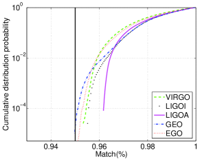
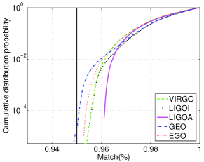
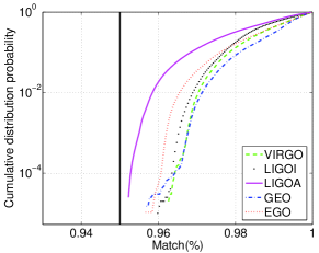
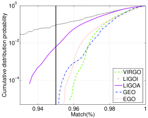
Figure 5: Cumulative efficiencies of the hexagonal template bank. Both template and signal are based on TaylorF2 model. From top left to bottom right (clockwise), injection and template bank cover the PBH binary, BNS, BHNS, and BBH inspiralling compact binaries.

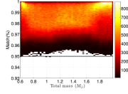
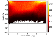
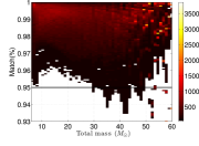
Figure 6: Efficiencies of the hexagonal template bank. Both template and signal are based on TaylorF2 model. From top left to bottom right (clockwise), injection and template bank cover the PBH binary, BNS, BHNS, and BBH inspiralling compact binaries.

IV.1 Description of the Physical Models

Theoretical calculations using post-Newtonian approximation of General Relativity give waveforms as expansions in the orbital velocity $v$, where $v=\left(2\pi Mf(t)\right)^{1/3}$. The PN expansions are known up to order $v^{5}$ in amplitude and $v^{7}$ in phase. However, we limit this study to restricted post-Newtonian, that is all amplitude corrections are discarded. Moreover, we expand the flux only to 2PN order. The energy function $E(v)$ and the flux $\mathcal{F}(v)$ are given by

$$E(v)=E_{N}\sum_{k}E_{k}v^{2k},\mathcal{F}(v)=\mathcal{F}_{N}\sum_{j}\mathcal{F}_{j}v^{j}.$$ (11)

We can obtain the phase starting from the kinematic equations $dt=(dt/dE)(dE/dv)dv$ and $d\phi/dt=2\pi f(t)$ and the change of binding energy $\mathcal{F}=-dE/dt$ giving a phasing formula of the form [25].

$$t(v) = t_{\rm ref}+m\int_{v}^{v_{\rm ref}}\,\frac{E^{\prime}(v)}{{\cal F}(v)}\,dv,$$

$$\phi(v) = \phi_{\rm ref}+2\int_{v}^{v_{\rm ref}}v^{3}\,\frac{E^{\prime}(v)}{{\cal F}(v)}\,dv\,.$$ (12)

There are different ways in which the above equations can be solved. For convenience, we introduce labels so as to refer to different physical template families that are used within the gravitational wave community and in our simulations.

TaylorT1

If we integrate the equations (12) numerically, we obtain the so-called TaylorT1 model. If instead, we use the P-approximant for the energy and flux functions [26, 21], then one generates the PadeT1 model.

TaylorT2

We can also expand $E^{\prime}(v)/\mathcal{F}(v)$ in a Taylor expansion in which case the integrals can be solved analytically to obtain the phase in terms of polynomial expressions as a function of $v$, which corresponds to TaylorT2 model [26]. This model is not used in this paper but results are very similar to the TaylorT3 model.

TaylorT3

From TaylorT2, $t(v)$ can be inverted and the polynomial expression of $v$ used within the expression for $\phi(v)$ to obtain an explicit time-domain phasing formula in terms of $t$. This corresponds to the TaylorT3 model.

EOB

The non-adiabatic models directly integrate the equations of motion (as opposed to using the energy balance equation) and there is no implicit conservation of energy used in the orbital dynamics approach [27, 28, 29, 21]. The EOB maps the real two-body conservative dynamics onto an effective one-body problem wherein a test mass moves in an effective background metric.

TaylorF2

The phasing formula is expressed in the Fourier domain, and is equivalent to the SPA case already mentioned.

IV.2 SPA Model Results

First, we validate the hexagonal template bank with a model based on the SPA (also labelled TaylorF2), used to compute the metric components. We set $\mathcal{\chi}_{s}=\mathcal{\chi}_{h}={\rm TaylorF2}$, and compute $\mathcal{E}$ and $\mathcal{S}_{\mathcal{R}}$. We intensively tested this bank by setting $N_{s}=200,000$ for each PSD and each parameter space considered. Using the template bank size from Table 2, the ratio $\mathcal{R}$ between template bank size and number of simulations varies from 1.7 to 375, which is much larger than unity in agreement with discussions that arose in Sec. II.3. The results are summarized in Fig. 5 and 6.

In Fig. 5, we notice that the hexagonal bank is efficient over the entire range of PBH binary, BNS, and BHNS searches. Moreover, the safeness is close to the minimal match ($\mathcal{S}_{\mathcal{R}}\in[95\%\textrm{--}96\%]$); by looking at the cumulative efficiencies, the bank seems to be neither under or over-efficient. However, looking more closely at $\mathcal{E}_{M}$ (see Fig. 6), we can identify a small over-efficient region in the BHNS case, where the efficiency is always larger than 97% for signals with total mass between $[4\textrm{--}20]M_{\odot}$.

In the BBH case, the bank is also efficient for the various PSDs with total mass between $[6-40]M_{\odot}$, and similarly to the BHNS case, it is over-efficient (above 97%) for systems with total mass between $[8\textrm{--}20]M_{\odot}$. The bank is also under-efficient with matches as low as 93% but for very high mass systems above $40~{}M_{\odot}$. The match below the minimal match are related to the LIGO-I PSD only, for which the lower cut-off frequency is 40 Hz. For high mass and nearly equal mass systems, the waveforms tend to be very short and contain only a few cycles: the metric is not a good approximation anymore. It also explains the feature seen at high mass, that shows some oscillations in the matches: a single template matches with many different injected signals. One solution to prevent matches to drop below the minimal match is to refine the grid for high mass range by decreasing the distances (i.e, increasing $MM$) between templates in this part of the parameter space. However, the high mass also correspond to the shortest waveforms which lead to a high rate of triggers in real data analysis. Therefore it is advised not to over-populate the high mass region. Overall, the hexagonal placement has the same behavior as in [12] but the bank is not over-efficient anymore in most cases.

IV.3 Non SPA Model Results

The square and hexagonal template banks are designed for TaylorF2 model. Yet, models presented in Section IV.1 do not differ from each other significantly so long as $v\ll c$, which is the case for PBH, BNS waveforms and most of the BHNS and BBH waveforms. Therefore, we expect the efficiencies of the template banks to be equivalent to the SPA-model results.

The models used in this Section have the same PN-order (i.e., 2PN) as in the TaylorF2 model. The simulation parameters are identical except the number of simulations that is restricted to $N_{s}=10,000$ for computational reasons. Finally, we tested only the BNS, BHNS and BBH searches. The PBH using SPA model being sufficient for a detection search.

IV.3.1 TaylorT1, TaylorT3, PadeT1

The TaylorT1, TaylorT3 and PadeT1 models give very similar results that are summarized in the Fig. 7, 8 and 9. The safeness is greater than the minimal match for the BNS and BHNS searches, for all three waveforms. More precisely, $\mathcal{S}_{\mathcal{R}}\approx 95\%$ for BNS case, and it is slightly over-efficient for BHNS case for total mass above $20~{}M_{\odot}$, especially in the case of PadeT1 model. In the BBH case, the bank is efficient between $[6\textrm{--}45]~{}M_{\odot}$. Then, matches drop to 93% for the same reason as in the case of SPA discussion. Therefore, we conclude that the proposed template bank is also efficient for TaylorT1, TaylorT3 and PadeT1 models.

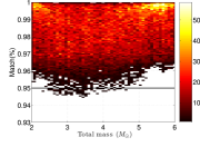
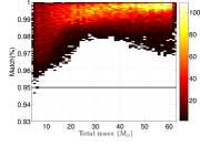
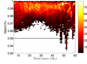
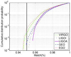
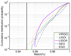
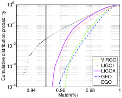
Figure 7: Hexagonal template bank efficiencies using TaylorT1 model. From left to right, results of the BNS, BHNS, and BBH injections.

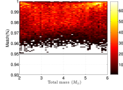
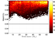
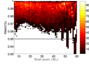
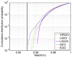
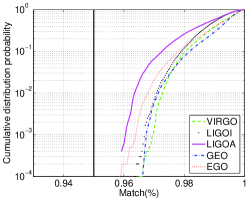
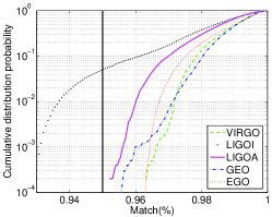
Figure 8: Hexagonal template bank efficiencies using TaylorT3 model. From left to right, results of the BNS, BHNS, and BBH injections.

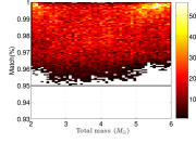
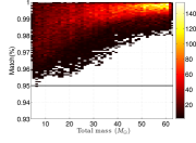
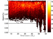
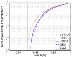
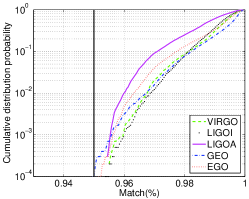
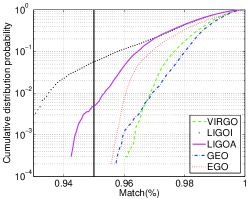
Figure 9: Hexagonal template bank efficiencies using PadeT1 model. From left ot right, results of the BNS, BHNS, and BBH injections.

IV.3.2 EOB

We also investigate the efficiency of the hexagonal template bank using EOB templates and signals. The EOB model is intrinsically different from the previous models. The results are summarized in Fig. 10. The safeness is slightly under the requested minimal match ($\mathcal{S}_{\mathcal{R}}=94.5\%\approx 95\%$). The template bank is efficient for BNS, BHNS and BBH cases. There is no over-efficiency noticed in any of the mass range considered. We can also notice that the cumulative $\mathcal{E}_{M}$ drops quickly and therefore we think that the proposed bank can be used with EOB model as well.

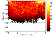
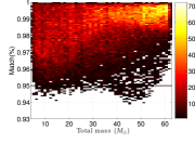
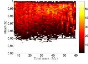
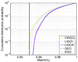
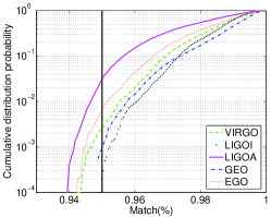
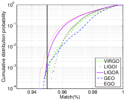
Figure 10: Hexagonal template bank efficiencies using EOB model. From left ot right, results of the BNS, BHNS, and BBH injections.

V Discussion and Conclusions

In this paper, we described a hexagonal template bank placement for the search of non-spinning inspiralling compact binaries in ground-based interferometers such as LIGO. The placement is based on a metric computed on the signal manifold of a stationary phase approximation model. The proposed hexagonal template bank size is about 40% smaller than the square template placement that was previously used to analyze LIGO science runs (i.e., [19]). Yet, the matches between signal and templates are above the required minimal match. Therefore, the template bank described in this paper is not over-efficient: it behaves as required. The main consequence is a reduction of 40% of the computational cost required to search for inspiralling compact binaries with respect to previous searches.

The proposed template bank is not unique. Several parameters can be tuned such as the sampling frequency, the final frequency used in the computation of the moments, the placement of the template along one eigen-vector or the other, each of which can be investigated in more detail.

The bank was tested with the aid of many simulations that use design sensitivity curves for advanced and current detectors, and various inspiralling compact binaries with total mass between $[0.6\textrm{--}63]M_{\odot}$. We used a model based on stationary phase approximation and showed that the template bank is efficient for most of the parameter space considered. The higher end of the mass range was slightly under efficient in the BBH case but this is partly related to the shortness of the signal and templates considered.

The proposed template bank can be used for various template families, not only the stationary phase approximation family. In particular, we tested the TaylorT1, TaylorT3, PadeT1, and EOB models at 2PN order, that have been used for simulated injections in the various LIGO science runs. It is interesting to see that the proposed template bank is efficient for most of the models considered in this paper. It is also worth noticing that in some cases the template bank is still over-efficient even though the bank size is already reduced by 40% (e.g., high mass BHNS injections).

The models that have been investigated in this paper are all based on 2PN order, therefore template families based on higher PN-order should be investigated. In the future, we also plan to consider the case of amplitude corrected waveforms. All simulations presented in this paper use the same model for both the template and signal generation. It would be interested to see how the template bank performs when templates are based on one model (say, Padé) and the signals are from another (say, EOB).

This hexagonal template bank is currently used within the LIGO project to search for non-spinning inspiralling compact binaries in the fifth science run.

Appendix A Detector’s Power Spectral Densities

The simulations that we performed use different PSD curves that are used to compute the inner products (Eq. 1). The different expressions provided uses the quantity $x=f/f_{0}$, where $f$ is the frequency and $f_{0}$ is a constant. We summarize the different design sensitivity curves that have been used in our simulations together with the lower cut-off frequency $f_{L}$:

• The EGO PSD [22] is given by

  $$\begin{split}S_{h}(f)=&S_{0}\left\{x^{p_{1}}+a_{1}x^{p_{2}}+\frac{}{}\right.\\ &\left.a_{2}\frac{1+b_{1}x+b_{2}x^{2}+b_{3}x^{3}+b_{4}x^{4}+b_{5}x^{5}+b_{6}x^{6}}{1+c_{1}x+c_{2}x^{2}+c_{3}x^{3}+c_{4}x^{4}}\right\}\end{split}$$ (13)

  where $S_{0}=1.61\times 10^{-51}$ and $f_{0}=200$ Hz. The other parameters are :
  $p_{1}=-4.05$, $p_{2}=-0.69$, $a_{1}=185.62$, $a_{2}=232.52$, $b_{1}=31.184$, $b_{2}=-64.72$, $b_{3}=52.24$, $b_{4}=-42.16$, $b_{5}=10.17$, $b_{6}=11.53$, $c_{1}=13.58$, $c_{2}=-36.46$, $c_{3}=18.56$, and $c_{4}=27.43$.

  The lower cut-off frequency is $f_{L}=20$ Hz.

• The GEO PSD is given by [30]

  $$\begin{split}S_{h}(f)&=S_{0}\left\{10^{-46}x^{-30}+34x^{-1}+\frac{}{}\right.\\ &\left.20\frac{\left[1-x^{2}+0.5x^{4}\right]}{1+0.5x^{2}}\right\}\end{split}$$ (14)

  where $S_{0}=10^{-46}$ and $f_{0}=150$ Hz. The lower cut-off frequency is $f_{L}=40$ Hz.

• The LIGO-I PSD [30] is given by

  $$\begin{split}S_{h}(f)&=S_{0}\left\{(4.49x)^{-56}+\right.\\ &\left.0.16x^{-4.52}+0.52+0.32x^{2}\right\},\end{split}$$ (15)

  where $S_{0}=9\times 10^{-46}$ and $f_{0}=150$ Hz. The lower cut-off frequency is $f_{L}=40$ Hz.

• The advanced LIGO PSD is based on data provided in [30] and given by

  $$\begin{split}S_{h}(f)&=S_{0}\left\{x^{-4.14}-5x^{-2}+\right.\\ &\left.111\left(\frac{1-x^{2}+0.5x^{4}}{1+0.5x^{2}}\right)\right\},\end{split}$$ (16)

  where $S_{0}=10^{-49}$ and $f_{0}=215$ Hz. The lower cut-off frequency is $f_{L}=20$ Hz.

• Finally, the VIRGO PSD is based on data provided by J-Y. Vinet and is approximated by

  $$S_{h}(f)=S_{0}\left\{(7.87x)^{-4.8}+\frac{6}{17}x^{-1}+\left(1+x^{2}\right)\right\},$$ (17)

  where $S_{0}=10.2\times 10^{-46}$ with $f_{0}=500$ Hz. The lower cut-off frequency is $f_{L}=20$ Hz.

Appendix B Parameter Space Tools

B.1 Basic Relations

Here is a summary of the relationship between individual masses $m_{1},\;m_{2}$, and the two chirptime parameters $\tau_{0}$ and $\tau_{3}$, that are given by

$$\tau_{0}=\frac{5}{256\pi f_{L}\eta}\left(\pi Mf_{L}\right)^{-5/3},\ \ \tau_{3}=\frac{1}{8f_{L}\eta}\left(\pi Mf_{L}\right)^{-2/3},$$ (18)

where $f_{L}$ is the lower cut-off frequency of the template/signal, $M=m_{1}+m_{2}$, and $\eta=m_{1}m_{2}/M^{2}$. The inversion is straightforward; $M$ and $\eta$ are given by

$$M=\frac{5}{32\pi^{2}f_{L}}\frac{\tau_{3}}{\tau_{0}},\ \ \eta=\frac{1}{8f_{L}\tau_{3}}\left(\frac{32\pi\tau_{0}}{5\tau_{3}}\right)^{2/3}.$$ (19)

It is convenient to introduce the constants $A_{0}$ and $A_{3}$ given by

$$A_{0}=\frac{5}{256\left(\pi f_{L}\right)^{8/3}},\ \ A_{3}=\frac{\pi}{8\left(\pi f_{L}\right)^{5/3}}\;,$$ (20)

so that Eq. 18 becomes

$$\tau_{0}=\frac{A_{0}}{\eta}M^{-5/3},\ \ \tau_{3}=\frac{A_{3}}{\eta}M^{-2/3}\;.$$ (21)

Finally, the chirp mass, $\mathcal{M}$, is given by

$$\mathcal{M}=\eta^{3/5}M$$ (22)

that allow $\tau_{0}$ to be expressed as a function of chirp mass only:

$$\tau_{0}=A_{0}\mathcal{M}^{-5/3}.$$ (23)

B.2 Parameter Space Boundaries relations

The parameter space is defined by three boundaries (see Fig. 1). On each of these boundaries, we want to express $\tau_{3}$ as a function of $\tau_{0}$. Using 21, we can eliminate $M$ and express $\tau_{3}$ as a function of $\tau_{0}$ and $\eta$:

$$\tau_{3}=\frac{A_{3}}{\eta}\left(\frac{\eta\tau_{0}}{A_{0}}\right)^{2/5}.$$ (24)

We can also eliminate $\eta$, and express $\tau_{3}$ as a function of $\tau_{0}$ and $M$:

$$\tau_{3}=\frac{A_{3}}{A_{0}}\tau_{0}M.$$ (25)

The lower boundary corresponds to $m_{1}=m_{2}$, or $\eta=1/4$. Using Eq. 24, we can express $\tau_{3}$ as a function of $\tau_{0}$ only

$$\tau_{3}=\left[4A_{3}\left(\frac{\tau_{0}}{4A_{0}}\right)^{2/5}\right]_{\eta=1/4}.$$ (26)

The second boundary is defined by $m_{1}=m_{\rm min}$ and $m_{2}$ in $[m_{\rm min}-m_{\rm max}]$. The third boundary is defined by $m_{1}=m_{\rm max}$ and $m_{2}$ in $[m_{\rm min}-m_{\rm max}]$. On those two boundaries, we can assume that $m_{1}$ is set to one of the extremity of the mass range, denoted $m_{\rm e}$. Then $m_{2}=M-m_{\rm e}$, and $\eta=(Mm_{\rm e})/(M-m_{\rm e})^{2}$. Starting from

$$\tau_{0}=\frac{A_{0}}{\eta}\left(M\right)^{-5/3},$$ (27)

we replace $\eta$ by its expression as a function of $M$ and $m_{\rm e}$, and obtain after some algebra a cubic equation of the form

$$x^{3}-px+q=0$$ (28)

where $x=M^{1/3}$, $p=-A_{0}/(\tau_{0}/m_{\rm e})$ and $q=-m_{\rm e}=0$, where $m_{\rm e}$ is either set to $m_{\rm Min}$ or $m_{\rm Max}$ depending on which side of the parameter space we are. The solution for $x$ is standard and is given by

$$x = \left(-\frac{q}{2}-\frac{1}{2}\sqrt{\frac{27q^{2}+4p^{3}}{27}}\right)^{\frac{1}{3}}+$$

$$\left(-\frac{q}{2}+\frac{1}{2}\sqrt{\frac{27q^{2}+4p^{3}}{27}}\right)^{\frac{1}{3}}$$

We replace, $M=x^{3}$ in Eq. 25 to obtain the value of $\tau_{3}$ on the boundaries when $\tau_{0}$ is provided.

Appendix C Flow Chart of the Hexagonal Placement Algorithm

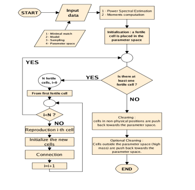
Figure 11: Flow chart of the hexagonal placement algorithm. See the text for detailled description of the initialization, reproduction, and connection process.