Multiresolution techniques for the detection of gravitational-wave bursts

Abstract

We present two search algorithms that implement logarithmic tiling of the time-frequency plane in order to efficiently detect astrophysically unmodeled bursts of gravitational radiation. The first is a straightforward application of the dyadic wavelet transform. The second is a modification of the windowed Fourier transform which tiles the time-frequency plane for a specific $Q$. In addition, we also demonstrate adaptive whitening by linear prediction, which greatly simplifies our statistical analysis. This is a methodology paper that aims to describe the techniques for identifying significant events as well as the necessary pre-processing that is required in order to improve their performance. For this reason we use simulated LIGO noise in order to illustrate the methods and to present their preliminary performance.

and

1 Introduction

Gravitational wave bursts[1] are short (less than one second) transients of gravitational radiation with poorly known waveforms. They are one of the distinct types of signals LIGO[2] and other interferometric and resonant mass detectors[3] are pursuing.

A search for such signals is generally a time-frequency search, since time and frequency information of the candidate events are essential for a multi-detector coincidence analysis as well as for relating events to astrophysical sources. One of the well established tools for such an analysis is the short time Fourier transform (also known as the windowed Fourier transform) developed by Denis Gabor in 1946. This approach applies standard Fourier transforms to short windowed segments of the original time series to create a uniform time-frequency map with a time resolution and frequency resolution that depends upon the window’s duration. However, it is impossible to pick a window duration appropriate for all frequencies. Low frequency signals require long duration windows to accumulate sufficient frequency information, while high frequency signals are better isolated in time using short duration windows. Time and frequency localization of transient signals is therefore not easily achieved with the short time Fourier transform. Here we have also assumed that burst waveforms are limited in $Q$; that is, that the number of oscillations fall within a particular range regardless of frequency.

In this introductory methods paper we explore multiresolution techniques for the detection of transients that rely on the dyadic wavelet transform[4, 5] and the constant $Q$ transform[6, 7]. Both methods search for a statistically significant excess of signal power in the time-frequency plane. However, contrary to existing excess power searches[8, 9, 10, 11], we implement a bank of filters that produce a logarithmic tiling of the time-frequency plane. This provides increasing time resolution at higher frequencies and thus naturally addresses the time-frequency localization problem.

This paper outlines these new methods and is organized as follows. Section 2 defines a representation independent parameterization of gravitational-wave bursts and defines an optimal signal to noise ratio, which motivates our use of a multiresolution approach. Section 3 presents the basics of the continuous and discrete wavelet transforms, while Section 4 presents the continuous and discrete $Q$ transform as a modification of the short time Fourier transform. Section 5 demonstrates how linear prediction can be used to whiten background noise prior to transform analysis. Section 6 describes methods for the selection of significant events from the output of the proposed algorithms, and Section 7 presents preliminary detection efficiencies of our search algorithms applied to Gaussian and sine-Gaussian bursts injected into simulated LIGO detector noise. Tuning and application of the proposed algorithms to search for a broader set of signals in data from the first LIGO science runs is currently in progress.

2 Gravitational-Wave Bursts

To further motivate the development of multiresolution techniques, we first consider the parameterization and detectability of gravitational-wave bursts that are well localized in both time and frequency. The more general case of non-localized bursts can be treated as a superposition of localized bursts.

2.1 The Parameterization of Gravitational-Wave Bursts

An arbitrary gravitational wave burst may be represented in both the time-domain and the frequency-domain by the Fourier transform pair $h(t)$ and $\tilde{h}(f)$. For bursts that are square-integrable, we may also define a representation independent characteristic squared amplitude,

$$\|h\|^{2}=\int_{-\infty}^{+\infty}|h(t)|^{2}\,dt=\int_{-\infty}^{+\infty}|\tilde{h}(f)|^{2}\,df.$$ (1)

For bursts that are well localized in both time and frequency, it is then meaningful to define a central time, central frequency, duration, and bandwidth:

$$t_{c} =\int_{-\infty}^{+\infty}t\frac{|h(t)|^{2}}{\|h\|^{2}}\,dt\qquad\qquad\sigma_{t}^{2} =\int_{-\infty}^{+\infty}(t-t_{c})^{2}\frac{|h(t)|^{2}}{\|h\|^{2}}\,dt$$ (2)

$$f_{c} =2\int_{0}^{\infty}f\frac{|\tilde{h}(f)|^{2}}{\|h\|^{2}}\,df\qquad\qquad\sigma_{f}^{2} =2\int_{0}^{\infty}(f-f_{c})^{2}\frac{|\tilde{h}(f)|^{2}}{\|h\|^{2}}\,df.$$ (3)

It can be shown that the duration and bandwidth, when defined in this way, obey an uncertainty relation of the form,

$$\sigma_{t}\sigma_{f}\geq\frac{1}{4\pi},$$ (4)

which we will also take as an approximate criterion for bursts that are well localized in the time-frequency plane. Finally, we define the dimensionless quality factor of a burst,

$$Q=f_{c}/\sigma_{f},$$ (5)

which for well localized bursts, is simply a measure of the burst’s aspect ratio in the time-frequency plane.

2.2 The Detectability of Gravitational-Wave Bursts

In general, a search algorithm for gravitational-wave bursts projects the data under test onto a basis constructed to span the space of plausible bursts. The optimal measurement occurs when a member of this basis exactly matches a gravitational-wave burst. In this case we achieve a signal to noise ratio, $\rho$, which for narrowband bursts or a flat detector noise spectrum, is simply the ratio of the total energy content of the signal, $\|h\|^{2}$, to the in-band one-sided power spectral density, $S_{h}(f)$, of the detector noise:

$$\rho^{2}=\int_{0}^{\infty}\frac{2|\tilde{h}(f)|^{2}}{S_{h}(f)}\,df\simeq\frac{\|h\|^{2}}{S_{h}(f)}.$$ (6)

Thus, $\|h\|$, which has units of strain per square root Hz, is a convenient quantity for evaluating the detectability of narrowband bursts since it is directly comparable to the amplitude spectral density of detector noise.

It is important to note, however, that the above signal to noise ratio is only achieved when a member of the measurement basis closely matches the signal in the time-frequency plane. Otherwise, the measurement encompasses either too little signal or too much noise, resulting in a loss in the measured signal to noise ratio. Since bursts are naturally characterized by their $Q$, we therefore choose to tile the time frequency plane by selecting a measurement basis which directly targets bursts within a finite range of $Q$. This naturally leads to a logarithmic tiling of the time frequency plane in which individual measurement pixels are well localized signals, all with the same $Q$.

3 The Wavelet Transform

3.1 The Continuous Wavelet Transform

In the preceding section, we motivate a search for bursts which projects the data under test onto a basis of well localized bursts of constant $Q$. The Wavelet transform[5] by construction satisfies these requirements, and is defined by the integral,

$$W_{f}(u,s)=\int_{-\infty}^{+\infty}f(t)\,\frac{1}{\sqrt{s}}\,\psi^{\star}\left(\frac{t-u}{s}\right)\,dt,$$ (7)

where the wavelet, $\psi$, is a time-localized function of zero average.

The coefficients $W_{f}(u,s)$ are evaluated continuously over times, $u$, and scales, $s$. Our ability to resolve in time and frequency is then determined by the properties $\psi$ assumes at each scale. At large scale, $\psi$ is highly dilated yielding improved frequency resolution at the expense of time resolution. At small scale, we achieve good time resolution with large uncertainty in frequency. However, since the number of oscillations is fixed, the resulting $Q$ is constant over all scales.

3.2 The Discrete Dyadic Wavelet Transform

For the case of discrete data, a computationally efficient algorithm exists for calculating wavelet coefficients over scales that vary as powers of two: $s\in\{2^{j-1}\,|\,j\in\mathbb{Z}^{+}\}$. This is the dyadic wavelet transform, which can be implemented for a limited family of wavelets using conjugate mirror filters. The filters consist of a high pass filter, $\hat{H}$, and low pass filter, $\hat{L}$, which can be applied in a cascade to obtain the wavelet coefficients. Beginning with the original time series, $A_{0}$, of length $N$, two sequences of length $N/2$ are obtained by application of the high pass and low pass filters followed by down-sampling. The sequence of detail coefficients, $D_{j}$, and approximation coefficients, $A_{j}$, are defined at each level, $j$, of the decomposition by

$$D_{j}=\hat{H}(A_{j-1})\hfill\mbox{and}\hfill A_{j}=\hat{L}(A_{j-1}).\hskip 72.26999pt$$ (8)

The detail coefficients for scale $s$, where $s=2^{j-1}$, calculated in this manner are the same as the wavelet coefficients obtained from Equation 7. If $N$ is a power of two, so that $N=2^{m}$, the final approximation sequence will be $A_{m}$.

The simplest dyadic wavelet is the Haar function:

$$\psi^{\mbox{\scriptsize Haar}}(t)=\left\{\begin{array}[]{rl}1&0\leq t<1/2\\ -1&1/2\leq t<1\\ 0&\mbox{otherwise.}\end{array}\right.$$ (9)

The corresponding high pass and low pass filters are

$$\hat{H}^{\mbox{\scriptsize Haar}}=[+1,-1]/\sqrt{2}\hfill\mbox{and}\hfill\hat{L}^{\mbox{\scriptsize Haar}}=[+1,+1]/\sqrt{2},\hskip 36.135pt$$ (10)

from which we see that the detail coefficients are related to the differences of each pair of points in the parent series, while the approximation coefficients are related to the averages of each pair.

A technique called wavelet packets can be used to further decompose the detail coefficients into smaller frequency subbands of higher $Q$. The Waveburst[11] search method currently implements a full wavelet packet decomposition which results in a uniform time-frequency plane with time-frequency cell sizes equivalent to those of the highest scale in the dyadic decomposition. It is possible, however, to choose a different subset of the wavelet packet coefficients which approximate a more constant $Q$ time-frequency plane by further decomposing the detail coefficents only a constant number of times at each scale. This would give much more flexibility to detect high $Q$ signals which do not match well to the mother wavelet $\psi$.

4 The $Q$ Transform

The $Q$ transform is a modification of the standard short time Fourier transform in which the analysis window duration varies inversely with frequency. It is similar in design to the continuous wavelet transform and also permits efficient computation for the case of discrete data. However, since reconstruction of the data sequence is not a concern, we permit violation of the zero mean requirement. In addition, the discrete $Q$ transform is not constrained to frequencies which are related by powers of two.

4.1 The Continuous Q Transform

We begin by projecting the sequence under test, $x(t)$, onto windowed complex sinusoids of frequency $f$:

$$x(\tau,f)=\int_{-\infty}^{+\infty}x(t)w(t-\tau,f)e^{-i2\pi ft}\,dt.$$ (11)

Here $w(t-\tau,f)$ is a time-domain window centered on time $\tau$ with a duration that is inversely proportional to the frequency under consideration[6, 7]. The $Q$ transform may also be expressed in an alternative form[6], which allows for efficient computation.

$$x(\tau,f)=\int_{-\infty}^{+\infty}\tilde{x}(\phi+f)\tilde{w}^{*}(\phi,f)e^{+i2\pi\phi\tau}\,d\phi.$$ (12)

Thus, the $Q$ transform at a specific frequency is obtained by a standard Fourier transform of the original time series, a shift in frequency, multiplication by the appropriate frequency domain window function, and an inverse Fourier transform. The benefit of Equation 12 is that the Fourier transform of the original time series need only be computed once. We then perform the inverse Fourier transform only for the logarithmically spaced frequencies that we are interested in.

4.2 The Discrete Q Transform

We may also adapt the $Q$ transform to the case of discrete data. In this case, Equation 11 takes the form:

$$x[m,k]=\sum_{n=0}^{N-1}x[n]w[n-m,k]e^{-i2\pi nk/N}.$$ (13)

As was the case for the continuous $Q$ transform, we may express the discrete $Q$ transform in the alternative form:

$$x[m,k]=\sum_{l=0}^{N-1}\tilde{x}[l+k]\tilde{w}^{*}[l,k]e^{+i2\pi ml/N}.$$ (14)

This allows us to take advantage of the computational efficiency of the fast Fourier transform for both the initial transform as well as the subsequent inverse transforms for each desired value of $k$.

Due to the implementation of the discrete $Q$ transform in Equation 14, the window function is most conveniently defined in the frequency domain. In particular, we choose a frequency domain Hanning window, which has finite support in the frequency domain while still providing good time-frequency localization.

5 Adaptive whitening by linear prediction

In this section, we present linear prediction[12, 13, 16, 17] as a tool for whitening gravitational-wave data prior to analysis by both the dyadic wavelet transform and the discrete $Q$ transform. For both transforms, the statistical distribution of transform coefficients is well known for the case of input white noise. Whitened data therefore permits a single predefined test for significance, which greatly simplifies the subsequent identification of candidate bursts. We also note that linear predictive whitening is a necessary component of current cross-correlation[14, 15] and time-domain[18] searches for gravitational-wave bursts in LIGO data.

Linear prediction assumes that the $n^{\mbox{\scriptsize th}}$ sample of a sequence is well modeled by a linear combination of the previous $M$ samples. We thus define the predicted sequence,

$$\hat{x}[n]=\sum_{m=1}^{M}c[m]x[n-m],$$ (15)

and the corresponding prediction error sequence,

$$e[n]=x[n]-\hat{x}[n].$$ (16)

The coefficients $c[m]$ are then chosen to minimize the mean squared prediction error,

$$\sigma_{e}^{2}=\frac{1}{N}\sum_{n=1}^{N}|e[n]|^{2},$$ (17)

over a representative training sequence of length $N$. Assuming that $x[n]$ is a stationary stochastic process, this results in the well known Yule-Walker[12] equations,

$$\sum_{k=1}^{M}r[m-k]c[m]=r[k]\qquad\mbox{for}\qquad 1\leq k\leq M,$$ (18)

where $r[k]$ is the autocorrelation of the training sequence $x[n]$ evaluated at lag $k$. In practice, we choose the biased autocorrelation estimate,

$$r[k]=\frac{1}{N}\sum_{n=|k|}^{N}x[n]x[n-|k|],$$ (19)

which guarantees the existence of a solution to the Yule-Walker equations.

When this process is applied to gravitational-wave data, the resulting prediction error sequence is composed primarily of sample to sample uncorrelated white noise. However, it also contains any unpredictable transient signals which were present in the original data sequence. Thus, the prediction error sequence is the whitened data sequence which we desire to subject to further analysis by the algorithms proposed in this paper. We therefore define the linear predictor error filter as the $M^{\mbox{\scriptsize th}}$ order finite impulse response filter, which when applied to a data sequence, $x[n]$, returns the corresponding prediction error sequence, $e[n]$:

$$e[n]=\sum_{m=0}^{M}b[m]x[n-m].$$ (20)

The choice of the filter order, $M$, is then determined by the measurement resolution of subsequent analysis. For a given filter order, the resulting prediction error sequence will be uncorrelated on time scales shorter than $M$ samples. In the frequency domain, this corresponds to a spectrum which is white on frequency scales greater than a characteristic bandwidth,

$$\Delta f\gtrsim\frac{f_{s}}{M},$$ (21)

where $f_{s}$ is the sample frequency of the data. Thus, we can whiten to any desired frequency resolution by selecting the appropriate filter order, $M$. In practice, we simply choose the minimum filter order which is sufficient for the subsequent analysis. For the training length, $N$, we choose to train over times which are long compared to the typical gravitational-wave bursts we are searching for.

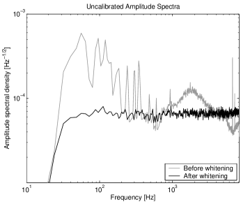
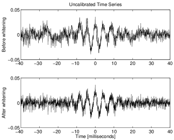
Figure 1: Example application of zero-phase linear predictive whitening to 48 seconds of sample uncalibrated gravitational-wave data from the second LIGO science run. In this case, the data was first high pass filtered at 64 Hz. A linear prediction error filter with 4 Hz whitening resolution was then trained on the first 16 seconds of data and applied to the subsequent 32 seconds of data. The ability of this process to whiten the data is evident in the left hand plot which shows the amplitude spectra of the data before and after whitening, when measured with an 8 Hz resolution in accordance with Equation 21. In addition, the right hand plot shows the effect of the same linear prediction error filter when applied to a simulated gravitational-wave burst injected into the data. In this case, we inject a 235 Hz sine-Gaussian with a $Q$ of 12.7 and signal to noise ratio of 20 as described in Section 7. Note the absence of a time delay between the whitened and unwhitened burst.

In order to avoid timing errors due to the unspecified phase response of linear prediction error filters, we construct a new filter from the unnormalized autocorrelation of the original filter coefficients:

$$b^{\prime}[k]=\sum_{m=|k|}^{M}b[m]b[m-|k|].$$ (22)

While this new filter has the desired property of zero phase response[19], its magnitude response has been squared. In practice, the construction of the zero phase filter is carried out in the frequency domain, where it is also possible to take the square root of the resulting frequency domain filter before transforming back to the time domain. An example application of zero-phase linear prediction to sample gravitational-wave data and a simulated gravitational-wave burst is shown in Figure 1.

6 Event Selection

We now seek to identify statistically significant events in the resulting dyadic wavelet transform and discrete $Q$ transform coefficients.

6.1 Dyadic Wavelet Transform Event Selection

We assume that linear predictive whitening (Section 5) has been applied to the data prior to the dyadic wavelet transform. Then, according to the central limit theorem, for a sufficiently large scale, $j$, the wavelet coefficients, $D_{j}$, within the scale will approach a zero-mean Gaussian distribution with standard deviation $\sigma_{j}$. We therefore define the sequence of squared normalized coefficients, or normalized pixel energies at scale $2^{j}$,

$$E_{j}=D^{2}_{j}/\sigma^{2}_{j},$$ (23)

which is chi-squared distributed with one degree of freedom (Figure 2).

It is then simply a matter of thresholding on the energy of individual pixels, $\epsilon_{ij}\in E_{j}$, to identify statistical outliers. We may also choose to cluster nearby pixels to better detect bursts which deviate from the dyadic wavelet tiling of the time-frequency plane. For a randomly selected cluster $C$ of $N$ pixels, we define the total cluster energy,

$$E_{C}=\sum_{(i,j)\in C}{\epsilon_{ij}},$$ (24)

which is also chi-square distributed, but with $N$ degrees of freedom. It is therefore possible to select a threshold energy to achieve a desired white noise false event rate. Alternatively, sharp transients may also be detected by simply searching for vertical clusters of pixels within the top $P_{j}$ percent of pixel energies in each scale.

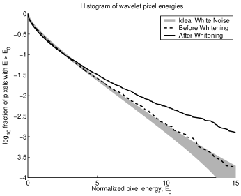
Figure 2: The distribution of dyadic wavelet transform (left) and discrete $Q$ transform (right) pixel energies in the scale and frequency bin encompassing 600 Hz for the data of Figure 1. The distributions before (dashed) and after (solid) linear predictive whitening are compared to the theoretically expected distributions for ideal white noise (shaded). The whitened data show good agreement with theory except at high pixel energy, where the unpredictable non-stationary behavior (glitches) of the gravitational-wave data becomes apparent. For the discrete $Q$ transform, the inconsistency of the unwhitened data with theoretical white noise is due to the coherent 600 Hz power line harmonic, which results in a Rician rather than exponential distribution of pixel energies. For the discrete Haar wavelet transform, the presence of a coherent signal results in an apparent, but false, white noise distribution. This is due to the use of a real valued wavelet which is sensitive to the relative phase between the signal and wavelet. This effect actually masks true non-stationarities, which are only exposed after linear predictive whitening removes the coherent signal content.

6.2 Discrete $Q$ Transform Event Selection

For the discrete $Q$ transform, we also make use of the central limit theorem by assuming that the data has first been whitened using linear prediction. For pixels of sufficiently long duration, the pixel energies,

$$\epsilon[m,k]=|x[m,k]|^{2},$$ (25)

at a particular frequency, $k$, will then approach an exponential distribution (Figure 2). Thus for each pixel, we have a measure of significance:

$$P(\epsilon>\epsilon[m,k])=\exp\left(-\epsilon[m,k]/\mu_{k}\right),$$ (26)

where $\mu_{k}$ is the mean pixel energy at frequency $k$. As with the discrete wavelet transform, we may also consider clusters of $N$ pixels and select a threshold energy in order to achieve a desired white noise false event rate. However in this case, the cluster energy is chi-square distributed with $2N$ degrees of freedom.

To efficiently detect bursts over a range of $Q$, we perform multiple $Q$ transforms, each of which produces a time-frequency plane tiled for a particular $Q$ within our range of interest. To best estimate the parameters of candidate bursts, we then select the most significant non-overlapping pixels among all $Q$ planes using a simple exclusion algorithm. Pixels are considered in decreasing order of significance and any pixel which overlaps in time or frequency with a more significant pixel is discarded. Thus, for each localized candidate burst, only the single pixel which best represents the burst parameters is reported. This does not exclude the possibility of clustering pixels from non-localized bursts, since the pixels which pass both the initial significance threshold as well as the exclusion algorithm will represent the strong localized features of such bursts. Reducing a non-localized burst to its strong, localized features has the additional benefit of a much tighter time-frequency coincidence criterion when multiple detectors are used.

7 Detection efficiencies over simulated LIGO noise

Finally, we evaluate the detection efficiencies of the proposed algorithms over simulated LIGO noise. The simulated data are composed of line sources and Gaussian distributed white noise passed through shaping filters to produce a power spectrum which matches the typical H1 detector noise spectrum during the second LIGO science run[21]. Assuming optimal orientation, we evaluate the detection efficiency for each waveform at various $\|h\|$ by injecting 256 such bursts at random times into the simulated data (see Figure 3). The simulated data are first filtered by a 6th order 64 Hz Butterworth high pass filter followed by a linear prediction error filter with whitening resolution of 16 Hz. However, we do not model the non-stationary behavior of real LIGO noise, which largely determines the false event rate of existing search algorithms. The algorithms considered in this paper are equally applicable to the identification of statistically significant transient events in auxiliary interferometer or environmental data. So, they may also prove useful for identifying potential vetoes.

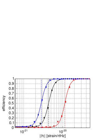
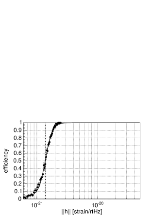
Figure 3: Detection efficiency versus injected characteristic strain amplitude for the dyadic wavelet transform (left) and the discrete $Q$ transform (right). The detection efficiency of the dyadic wavelet transform is shown for three durations of Gaussian bursts with $\sigma_{t}$’s of 0.35, 0.71, and 1.41 milliseconds as shown from left to right. The detection efficiency of the $Q$ transform is shown for a sine-Gaussian burst with a $Q$ of 12.7 and central frequency, $f_{c}$, of 275 Hz.

The low $Q$ Haar wavelet is best suited to broadband signals, and for a representative broadband waveform, we use Gaussian injections of the form $h(t)=h_{0}\exp(-t^{2}/4\sigma_{t}^{2})$, for $\sigma_{t}$’s of 0.35, 0.71, and 1.41 ms. The filtered data are passed through the discrete wavelet transform and event selection algorithm as described in Section 6.1 for a false event rate of 0.5 Hz. We allow clusters to be composed of a single pixel, or a combination of two pixels adjacent or overlapping in time and adjacent in scale for scales, $j$, of 5, 6, and 7. For $\sigma_{t}$’s of 0.35, 0.71, and 1.41 ms, we obtain 50% efficiencies for $\|h\|$ equal to $2.8\times 10^{-21}$, $4.4\times 10^{-21}$, and $1.1\times 10^{-20}$ Hz^-1/2, which correspond to signal to noise ratios, $\rho$, of 3.6, 3.7, and 3.5.

Since the discrete $Q$ transform targets well localized bursts, we demonstrate its efficiency for sine-Gaussian bursts of the form, $h(t)=h_{0}\exp(-t^{2}/4\sigma_{t}^{2})\sin(2\pi f_{c}t)$, with a $Q$ of 12.7 and central frequency, $f_{c}$, of 275 Hz. The discrete $Q$ transform is applied to the whitened data with approximately 75 percent pixel overlap to search for single pixel bursts within the frequency band 64–4096 Hz and with $Q$’s in the vicinity of 10.6, 14.1, and 17.7. Candidate events are then identified as described in Section 6.2 in order to obtain a 1 Hz white noise false rate. The resulting 50% detection efficiency occurs at an $\|h\|$ of $1.5\times 10^{-21}$ Hz^-1/2, corresponding to a $\rho$ of 3.0.

8 Conclusions

We have described two transient-finding algorithms using logarithmic tiling of the time-frequency plane and examined their applicability to the detection of gravitational wave bursts. The methods work more efficiently when data are whitened and for this we have introduced a data conditioning algorithm based on linear prediction. As a first step in quantifying their performance, we have used simulated noise data according to the LIGO noise spectra from its second science run. Moreover, ad hoc waveform morphologies were used to simulate the presence of a burst signal over the noise. This allowed us to measure the algorithms’ efficiency at a fixed false alarm rate of O(1Hz). The results are encouraging and we are continuing the computation for mapping the efficiency of the algorithms as a function of their false alarm rate.

Needless to say, even if the shaped LIGO noise with some line features that we used for our simulation is a step forward, it does remain unrealistic. Real interferometric data have richer line structure, non-stationary and non-gaussian character that may be far from our assumptions; at the same time though, it is extremely hard to simulate. All of these make the perfomance estimates that we made using our simulation model optimistic. The use though of mathematically well described noise allows the straightforward reproduction and comparison of our results with other methods. An end-to-end pipeline using the aforementioned methods for whitening and transient-finding on data collected by the LIGO instruments is currently in development. This will provide the ultimate test of the performance of the algorithms and will be reported separately within the context of the LIGO Scientific Collaboration (LSC) data analysis ongoing research.

This work was supported by the US National Science Foundation under Cooperative Agreement No. PHY-0107417.

References

References

- [1] Thorne K, 300 Years of Gravitation, (1987) Cambridge University Press.
- [2] Gonzalez G, Class. Quantum Grav., 21 (2004) S1575.
- [3] Thorne K, Proceedings of the Snowmass 95, (1995) World Scientific.
- [4] Daubechies I, Ten Lectures on Wavelets, (1992) SIAM.
- [5] Mallat S, A Wavelet Tour of Signal Processing, (1999) Academic Press.
- [6] Stockwell R, et al., IEEE Transactions on Signal Processing, 44(4) (1996) 998–1001.
- [7] Brown J, J. Acoust. Soc. Am., 89(1) (1991) 425–434.
- [8] Abbott B et al., Phys. Rev. D 69 (2004) 102001.
- [9] Anderson W et al., Phys. Rev. D 63 (2001) 042003.
- [10] Sylvestre J, Phys. Rev. D 66 (2002) 102004.
- [11] Klimenko S, Class. Quantum Grav., 21 (2004) S1819.
- [12] Makhoul J, Proc. IEEE 63 (1975) 561.
- [13] Haykin S, Adaptive Filter Theory, 4th Edition (2002) Prentice-Hall.
- [14] Cadonati L, Class. Quantum Grav., 21 (2004) S1695.
- [15] Mohanty S, Class. Quantum Grav., 21 (2004) S1831.
- [16] Cuoco E et al., Phys.Rev. D 64 (2001) 122002
- [17] Searle A et al., Class. Quantum Grav. 20 (2003) S721-S730
- [18] McNabb J et al., Class. Quantum Grav., 21 (2004) S1705.
- [19] Oppenheim A and Schafer R, Discrete-Time Signal Processing, (1989) Prentice-Hall.
- [20] Press W et al., Numerical Recipes in C, (1992) Cambridge University Press.
- [21] http://www.ligo.caltech.edu/∼lazz/distribution/LSC_Data/