Dynamics of a $\mathbb{Z}_{2}$ symmetric EdGB gravity in spherical symmetry

Abstract

We report on a numerical investigation of black hole evolution in an Einstein dilaton Gauss-Bonnet (EdGB) gravity theory where the Gauss-Bonnet coupling and scalar (dilaton) field potential are symmetric under a global change in sign of the scalar field (a “$\mathbb{Z}_{2}$” symmetry). We find that for sufficiently small Gauss-Bonnet couplings Schwarzschild black holes are stable to radial scalar field perturbations, and are unstable to such perturbations for sufficiently large couplings. For the latter case, we provide numerical evidence that there is a band of coupling parameters and black hole masses where the end states are stable scalarized black hole solutions, in general agreement with the results of Macedo et. al. [1]. For Gauss-Bonnet couplings larger than those in the stable band, we find that an “elliptic region” forms outside of the black hole horizon, indicating the theory does not possess a well-posed initial value formulation in that regime.

• July 2020

Keywords: modified gravity, numerical relativity

1 Introduction

The recent advent of the field of gravitational wave astronomy has led to increased interest in testing modifications/extensions of general relativity (GR) (e.g. [2]). This requires understanding the dynamics of those theories during binary black hole inspiral and merger. While perturbative solutions to modified gravity theories may be sufficient to describe their predictions during the inspiral phase, where the black holes are well separated and gravitational fields are relativity weak, the loudest signal during binary inspiral comes from the merger phase, where gravity is in the strong field, dynamical regime (e.g. [3]). Order reduction solutions to modified gravity theories offer a potential route to extracting predictions from those theories (e.g. [4, 5]). Solving the full equations of motion without using order reduction potentially offers certain advantages though, as in this approach one does not have to consider delicate issues (e.g. “secular effects”) regarding when the perturbative order-reduction approximation may fail. Motivated by this, here we consider the nonlinear spherical dynamics of a variant of Einstein dilaton Gauss-Bonnet (EdGB) gravity in spherical symmetry. While much of the relevant physics to gravitational wave astronomy (most importantly, gravitational waves) are not present in spherical symmetry, our study explores the dynamics of the scalar degree of freedom in the theory, which will be relevant when solving for the dynamics of the theory in less symmetrical spacetimes.

The variant of EdGB gravity we study has been shown to possess spherically symmetric scalarized black hole solutions that are stable to linear, radial perturbations [1]. We find numerical evidence that stable scalarized black holes can be formed in this theory, but for large enough Gauss-Bonnet coupling the theory dynamically loses hyperbolicity. Our results, along with the recent work of [6, 7], suggests that for sufficiently small couplings scalarized black hole solutions in this theory could be studied in binary inspiral and merger scenarios.

An outline of the remainder of the paper is as follows. In Sec.2 we describe the particular EdGB theory we consider, and the resulting equations of motion in spherical symmetry. In Sec.3 we briefly summarize earlier work on scalarized black holes in this theory. In Sec.4 we describe our numerical code. In Secs. 5 and 6 we describe our initial data and evolution results respectively. We present concluding remarks in Sec. 7. In A we describe the characteristic analysis we employ during evolution, contrasting it with linear perturbation analysis, and in B we derive the approximate scalarized initial data we used in some of our simulations.

We use geometric units ($8\pi G=1$, $c=1$) and follow the conventions of Misner, Thorne, and Wheeler [8].

2 Equations of motion

The action for the class of EdGB gravity theories we consider is

$$S=\int d^{4}x\sqrt{-g}\left(\frac{1}{2}R-\frac{1}{2}(\nabla\phi)^{2}-V(\phi)+W(\phi)\mathcal{G}\right),$$ (1)

where $\phi$ is a scalar field (the “dilaton” field), $g$ is the metric determinant, $V(\phi)$ and $W(\phi)$ are (so far unspecified) functions of $\phi$, $R$ is the Ricci scalar, and $\mathcal{G}$ is the Gauss-Bonnet scalar:

$$\mathcal{G}\equiv\frac{1}{4}\delta^{\mu\nu\alpha\beta}_{\rho\sigma\gamma\delta}R^{\rho\sigma}{}_{\mu\nu}R^{\gamma\delta}{}_{\alpha\beta},$$ (2)

where $\delta^{\mu\nu\alpha\beta}_{\rho\sigma\gamma\delta}$ is the generalized Kronecker delta tensor and $R^{\rho\sigma}{}_{\mu\nu}$ is the Riemann tensor. Varying 1 with respect to the metric and scalar fields, the EdGB equations of motion are

$$E^{(g)}_{\mu\nu} \equiv R_{\mu\nu}-\frac{1}{2}g_{\mu\nu}R+2\delta^{\gamma\delta\kappa\lambda}_{\alpha\beta\rho\sigma}R^{\rho\sigma}{}_{\kappa\lambda}\left(\nabla^{\alpha}\nabla_{\gamma}W(\phi)\right)\delta^{\beta}{}_{(\mu}g_{\nu)\delta}-T_{\mu\nu}=0,$$ (3a)

$$T_{\mu\nu} \equiv \nabla_{\mu}\phi\nabla_{\nu}\phi-g_{\mu\nu}\left[\frac{1}{2}(\nabla\phi)^{2}+V(\phi)\right],$$

$$E^{(\phi)} \equiv \nabla_{\mu}\nabla^{\mu}\phi-V^{\prime}(\phi)+W^{\prime}(\phi)\mathcal{G}=0,$$ (3b)

where the “prime” operation defines a derivative with respect to the scalar field $\phi$; e.g. $V^{\prime}(\phi)\equiv dV(\phi)/d\phi$. We see that if $\phi=const.$, then the Gauss-Bonnet scalar term does not contribute to the equations of motion; this is a consequence of the fact that the Gauss-Bonnet scalar is locally a total derivative in four dimensional spacetime (see e.g. [9]). In this article we will solve Eqs. 3a with the following choice for functions $V(\phi)$ and $W(\phi)$

$$V(\phi)= \frac{1}{2}\mu^{2}\phi^{2}+\lambda\phi^{4},$$ (3da)

$$W(\phi)= \frac{1}{8}\eta\phi^{2},$$ (3db)

where $\mu,\lambda$ and $\eta$ are constant parameters. In our earlier works on EDGB gravity we used the potentials $V=0,W=\lambda\phi$ [10, 11, 12]); that choice encompasses the leading order term for shift symmetric $\phi\to\phi+const.$ EdGB gravity models. Here, we focus on the form 3da and 3db, the leading order contributions to theories that have $\phi\to-\phi$ ($\mathbb{Z}_{2}$) symmetry [1]. We note that with the code we have developed we could in principle investigate the spherical dynamics of EdGB gravity theories with arbitrary functions $V(\phi)$ and $W(\phi)$ (see Sec. 4.1).

The potential $W(\phi)$ satisfies an “existence condition”for pure GR solutions [13]: at the minimum $\phi_{0}$ of the potential $W(\phi)$, here $\phi_{0}=0$, the potential satisfies:

$$W^{\prime}\big{|}_{\phi=0}=0.$$ (3de)

That is, for $W$ that obey Eq. 3de we can obtain dynamical GR solutions with $\phi=0$, as the $\phi$ will not be sourced by curvature (although it could still potentially be sourced by other matter fields, and once there are regions where $\phi\neq 0$, $W^{\prime}\neq 0$ and the scalar field could then be sourced by curvature terms).

We evolve this system in Painlevé-Gullstrand (PG)-like coordinates (e.g. [14, 15, 16, 17])

$$ds^{2}=-\alpha(t,r)^{2}dt^{2}+\left(dr+\alpha(t,r)\zeta(t,r)dt\right)^{2}+r^{2}\left(d\vartheta^{2}+\mathrm{sin}^{2}\vartheta d\varphi^{2}\right),$$ (3df)

so-named since $t={\rm const.}$ cross sections are spatially flat as in the PG coordinate representation of the Schwarzschild black hole (which in these coordinates is given by $\alpha=1,\zeta=\sqrt{2m/r}$).

We define the variables

$$Q\equiv \partial_{r}\phi,$$ (3dga)

$$P\equiv \frac{1}{\alpha}\partial_{t}\phi-\zeta Q=n^{\mu}\partial_{\mu}\phi,$$ (3dgb)

and obtain the following system of evolution equations for $\phi$, $Q$ and $P$:

$$E_{(\phi)}\equiv \partial_{t}\phi-\alpha\left(P+\zeta Q\right)=0,$$ (3dgha)

$$E_{(Q)}\equiv \partial_{t}Q-\partial_{r}\left(\alpha\left[P+\zeta Q\right]\right)=0,$$ (3dghb)

$$E_{(P)}\equiv \mathcal{A}_{(P)}\partial_{t}P+\mathcal{F}_{(P)}=0.$$ (3dghc)

The evolution equation for $\phi$ (Eq. 3dgha) follows from the definition of $P$ (Eq. 3dgb), and the evolution equation for $Q$ (Eq. 3dghb) follows from taking the radial derivative of Eq. 3dgha. The evolution equation for $P$ (Eq. 3dghc) comes from taking algebraic combinations of Eq. 3b and the $tr$, $rr$, and $\vartheta\vartheta$ components of Eq. 3a (c.f. [12]). The quantities $\mathcal{A}_{(P)}$ and $\mathcal{F}_{(P)}$ are lengthy expressions of $\{\alpha,\zeta,P,Q\}$ and their radial derivatives. In the limit $W=0$, Eq. 3dghc reduces to

$$\partial_{t}P-\frac{1}{r^{2}}\partial_{r}\left(r^{2}\alpha\left[Q+\zeta P\right]\right)+\alpha V^{\prime}=0.$$ (3dghi)

Interestingly, in PG coordinates the Hamiltonian and momentum constraints do not change their character as elliptic differential equations (or more properly, as ordinary differential equations in the radial coordinate $r$) going from GR to EdGB gravity:

$$E^{(g)}_{\mu\nu}n^{\mu}n^{\nu}\propto \left(1-\frac{8QW^{\prime}}{r}-\frac{12P\zeta W^{\prime}}{r}\right)\partial_{r}\zeta+\left(\zeta-\frac{8Q\zeta W^{\prime}}{r}-\frac{12P\zeta^{2}W^{\prime}}{r}\right)\frac{\partial_{r}\alpha}{\alpha}$$ (3dghja)

$$+\frac{\zeta}{2r}-\frac{r}{2\zeta}\rho-\frac{4W^{\prime}\zeta}{r}\partial_{r}Q-\frac{4W^{\prime\prime}Q^{2}\zeta}{r}=0,$$

$$E^{(g)}_{\mu r}n^{\mu}\propto \left(1-\frac{8W^{\prime}Q}{r}-\frac{8W^{\prime}P\zeta}{r}+\frac{4W^{\prime}Q\zeta^{2}}{r}\right)\frac{\partial_{r}\alpha}{\alpha}-\frac{r}{2\zeta}j_{r}$$ (3dghjb)

$$+\frac{4W^{\prime}\zeta}{r}\partial_{r}P+\frac{4W^{\prime}Q\zeta}{r}\partial_{r}\zeta+\frac{4W^{\prime\prime}PQ\zeta}{r}=0,$$

where

$$\rho \equiv n^{\mu}n^{\nu}T_{\mu\nu}=\frac{1}{2}\left(P^{2}+Q^{2}\right)+V,$$ (3dghjka)

$$j_{\kappa} \equiv -\gamma_{\kappa}{}^{\mu}n^{\nu}T_{\mu\nu}=-PQ,$$ (3dghjkb)

and $n_{\mu}\equiv(-\alpha,0,0,0)$.

3 Earlier work on $\mathbb{Z}_{2}$ symmetric EdGB gravity

Here we briefly review recent work on $\mathbb{Z}_{2}$ symmetric EdGB gravity theories. Potentials of the form $V=0$ and $W=w_{2}\phi^{2}$ were considered in [13]. There the authors found scalarized black hole solutions, which were subsequently found to be mode unstable to radial perturbations in [18]. Subsequently, radial mode-stable scalarized black hole solutions were found for couplings of the form $V=0$, $W=w_{2}\phi^{2}+w_{4}\phi^{4}$ in [19, 20]. Couplings of the form $V=0$ and $W=c_{0}+\mathrm{exp}\left(c_{e}\phi^{2}\right)$ have been investigated in [21, 18], and also give rise to radially stable scalarized black hole solutions.

The authors in [1] introduced the model we study in this article, $V=\mu^{2}\phi^{2}+2\lambda\phi^{4}$, $W=\eta\phi^{2}/4$. This model is motivated by effective field theory arguments: assuming the action is invariant under the $\mathbb{Z}_{2}$ symmetry $\phi\to-\phi$, the action contains all terms (except for the term $(\nabla\phi)^{4}$, which we do not consider in this article) of mass dimension equal to or less than the mass dimension of $\phi^{2}\mathcal{G}$, which is the lowest order term that couples $\phi$ to the Gauss-Bonnet scalar subject to this symmetry. Though like the authors in [1], while we motivate this model from effective field theory we in fact will treat the theory as a complete classical field theory, and consider exact (to within numerical truncation error) solutions to the equations of motion.

In [1], the authors found scalarized black hole solutions stable to linear radial perturbations for certain ranges of the dimensionless parameters

$$\hat{M}\equiv \frac{M}{\eta^{1/2}},$$ (3dghjkla)

$$\hat{\Phi}\equiv \frac{\Phi}{\eta^{1/2}},$$ (3dghjklb)

$$\hat{\mu}\equiv \mu\eta^{1/2},$$ (3dghjklc)

$$\hat{\lambda}\equiv \lambda\eta,$$ (3dghjkld)

where $M$ is the asymptotic mass of the black hole plus scalar field configuration and $\Phi$ is the asymptotic scalar “charge”, i.e. for scalarized black hole solutions to the theory it is the coefficient to the leading nonzero term in $\phi(t,r)$ as $r$ goes to infinity [1]

$$\lim_{r\to\infty}\phi(t,r)\sim e^{-\mu r}\left(\frac{1}{r}\Phi+\cdots\right).$$ (3dghjklm)

A nonzero value of $\hat{\lambda}$ is necessary to have radially linear mode stable scalarized black hole solutions, and the value of $\hat{\lambda}$ needed to stabilize a given scalarized black hole increases as $\hat{\mu}$ increases [1]. For example, when $\hat{\mu}=0$, the minimum value of $\hat{\lambda}\approx 0.2$. There is also a maximum value of $\hat{M}$ for a scalarized black hole (above this the Schwarzschild solution is stable); for example for $\hat{\mu}=0$, found this maximum to be $\hat{M}\approx 0.6$.

4 Description of code and simulations

4.1 Code description

Our basic evolution strategy is the same as in [11]: we freely evolve $P$ and $Q$ using Eqs. 3dghb and 3dghc, and solve for $\alpha$ and $\zeta$ using the constraint equations, Eqs. 3dghja and 3dghjb. The boundary condition for $\zeta$ at the excision boundary is obtained by freely evolving it using the $E_{tr}$ equation of motion (with algebraic combinations of the other equations of motion to remove time derivatives of $\alpha$ and $P$). We do not need to impose any boundary condition for $\alpha$ on the excision boundary due to the $\alpha\to\alpha+c(t)$ residual gauge symmetry in PG coordinates. The full equations of motion for $P$ and the freely evolved $\zeta$ on the boundary are long and unenlightening, although see Appendix C of [11] for their full form in PG coordinates for the special case $V=0$ (and note that there we use the notation $W\equiv f$).

As in [11], we solve the constraint equations using the trapezoid rule (a second order method) with relaxation. Unlike [11] though, we solve the evolution equations for $\{P,Q\}$, and $\zeta$ on the excision boundary using a fourth order method of lines technique: we use fourth order centered difference stencils to evaluate the spatial derivatives, and evolve in time with a fourth order Runge-Kutta integrator (e.g. [22, 23]). At the excision boundary and the boundary at spatial infinity we used one-sided difference stencils to evaluate spatial derivatives. We solve the equations over a single grid (unigrid evolution). An example of a convergence study with the independent residual $E_{rr}$ is shown in Fig. 3.

The code is written in C++, and can be accessed at [24].

4.2 Diagnostics

Our code diagnostics are as in [10, 11, 12], which we very briefly review here. The mass of a given simulation is determined by the value of the Misner-Sharp mass at spatial infinity:

$$m_{total}=\lim_{r\to\infty}m_{MS}(t,r)=\lim_{r\to\infty}\frac{r}{2}\zeta(t,r)^{2}.$$ (3dghjkln)

Another diagnostic we compute is the radial characteristic speed of the dynamical degree of freedom of EdGB gravity in spherical symmetry. To compute the radial characteristic speeds, we compute the characteristic vector $\xi_{a}$ by finding the zeros of the characteristic equation:

$$\mathrm{det}\left[\pmatrix{\delta E_{(P)}/\delta(\partial_{a}P)&\delta E_{(P)}/\delta(\partial_{a}Q)\cr\delta E_{(Q)}/\delta(\partial_{a}P)&\delta E_{(Q)}/\delta(\partial_{a}Q)}\xi_{a}\right]=0.$$ (3dghjklo)

and then compute the ingoing and outgoing characteristic speeds $c_{\pm}\equiv\mp\xi_{t}/\xi_{r}$. Expanding Eq. 3dghjklo gives us a quadratic equation for the radial characteristic speeds

$$\mathcal{A}c^{2}+\mathcal{B}c+\mathcal{C}=0,$$ (3dghjklp)

where $\mathcal{A}$, $\mathcal{B}$, and $\mathcal{C}$ are complicated functions of the metric and scalar fields, and their time and radial derivatives (c.f. [11]). The discriminant $\mathcal{D}\equiv\mathcal{B}^{2}-4\mathcal{A}\mathcal{C}$ determines the hyperbolicity of the theory at each spacetime point. Where $\mathcal{D}>0$, the radial characteristic speeds are real and the equations of motion for the theory at that spacetime point are hyperbolic. Where $\mathcal{D}<0$, the radial characteristic speeds are imaginary and the equations of motion for the system defined by Eq 3dgha, Eq 3dghb, and Eq 3dghc at that spacetime point are elliptic . We discuss the difference between computing the radial characteristics and computing the modes of radial linear perturbations about a stationary solution in A.

We determine the location of the black hole horizon in our simulation by computing the location of the marginally outer trapped surface (MOTS) for outgoing null characteristics [25]. In PG coordinates the radial null characteristics are

$$c^{(n)}_{\pm}=\alpha\left(\pm 1-\zeta\right),$$ (3dghjklq)

thus the location of the MOTS is at the point $\zeta(t,r)=1$.

5 Initial data

5.1 General considerations

We may freely specify $\phi$ and $\partial_{t}\phi$ (or, $\phi$ and $P$) on the initial data surface as $\phi$ satisfies a second order in time wave-like equation, provided the characteristics for that equation are real. The variables $\alpha$ and $\zeta$ must satisfy the constraint equations, and are not freely specifiable.

Note that $\phi=0,\partial_{t}\phi=0$ is not just a solution to the initial value problem for EdGB gravity with this coupling potential (3da and 3db), it is also a consistent solution to the full evolution equations (in fact this was one criterion used by the authors in [13] in constructing this model of EdGB gravity). This is in contrast to EdGB gravity with a linear shift-symmetric potential, where $\phi=0,\partial_{t}\phi=0$ can by imposed as an initial condition, but then $\phi$ will generically evolve to non-zero values with time.

5.2 Black hole initial data with a small exterior scalar pulse

Our class of initial data is similar to that we used in [11]: the free initial data is $\phi$ and $P$, from which we can determine $Q,\alpha,\zeta$. To have black hole initial data, at the initial excision boundary $x_{exc}$ we set

$$\alpha|_{x=x_{exc}}= 1,$$ (3dghjklr)

$$\zeta|_{x=x_{exc}}= \sqrt{\frac{2M}{r}},$$ (3dghjkls)

with $\phi$ and $P$ compactly supported away from the excision boundary, and then integrate outwards in $r$ to obtain $\alpha$ and $\zeta$ over the initial data surface. The quantity $M$ in Eq. 3dghjklr is the initial mass of the black hole.

We choose the following for the exterior scalar pulse

$$\phi_{b}(t,r)\big{|}_{t=0}= \cases{\frac{a_{0}}{n_{0}}\left(r-r_{l}\right)^{2}\left(r_{u}-r\right)^{2}\mathrm{exp}\left[-\frac{1}{r-r_{l}}-\frac{1}{r_{u}-r}\right]\qquad r_{l}<r<r_{u}\\ 0\qquad\mathrm{otherwise}},$$ (3dghjklta)

$$Q_{b}(t,r)\big{|}_{t=0}= \partial_{r}\phi(t,r)\big{|}_{t=0},$$ (3dghjkltb)

$$P_{b}(t,r)\big{|}_{t=0}= 0,$$ (3dghjkltc)

where $r_{u}>r_{c}>r_{l}>2M$, and the normalization $n_{0}$ is chosen such that

$$\max\phi_{b}(t,r)\Big{|}_{t=0}=a_{0}.$$ (3dghjkltu)

5.3 Approximate scalarized profile

We also consider initial data that approximates the static decoupled scalarized profile on a Schwarzschild black hole background (see also [1]):

$$\phi(t,r)\big{|}_{t=0}= \frac{\Phi_{0}}{r}\mathrm{exp}\left(-\mu\left(r-3M\right)\right),$$ (3dghjkltv)

$$Q(t,r)\big{|}_{t=0}= \partial_{r}\phi(t,r)\big{|}_{t=0},$$ (3dghjkltw)

where $\Phi_{0}$ is a constant; see Appendix B for a derivation. We choose $P$ so that $\partial_{t}\phi\approx 0|_{t=0}$ (see 3dgb): we set

$$P(t,r)\big{|}_{t=0}= -Q(t,r)\zeta(t,r)\big{|}_{t=0},$$ (3dghjkltx)

and initially set $\alpha=1$, $\zeta=\sqrt{2M/r}$. We then resolve the constraints for $\alpha$ and $\zeta$, set $P$ as above, and iterate this process until the maximum change in $P$, $|\Delta P|_{\infty}$, between iterations is less than $10^{-3}$.

6 Numerical results

We will only present results for $\eta>0$, and absorb $\eta$ into the definition of the dimensionless parameters (Eqs. 3dghjkla-3dghjkld). As one check of the code we did perform simulations with the GR case $\eta=0$; in these simulations some of the scalar field would fall into the black hole, and some of the field would disperse to infinity, leaving a vacuum Schwarzschild solution behind. This is consistent with the no hair theorems for a canonically coupled scalar field with a potential in asymptotically flat spacetimes (for a review and references see e.g. [26]), along with perturbative solutions of scalar fields around a Schwarzschild black hole background (for a review and references see e.g. [27]).

We find that for both classes of initial data described in the previous section, we can separate the solutions into three types: (1) the scalar field disperses, leaving behind a Schwarzschild black hole, (2) the black hole scalarizes and approaches a static solution, or (3) an elliptic region eventually forms outside the black hole (i.e. exterior to the apparent horizon).

6.1 Compact scalar pulse initial data

In Fig. 1 we show several points on a plot of $\hat{M}$ versus $\hat{\lambda}$ (for the definition of $\hat{M}$ and $\hat{\lambda}$ see respectively Eq. 3dghjkla and Eq. 3dghjkld), indicating the division between evolution that forms elliptic regions and that which does not, beginning from the compact pulse initial data described in Sec. 5.2. To arrive at the numerical data points in the figure, we fixed the initial data parameters $r_{l}$, $r_{u}$, and $a_{0}$ and black hole mass. Specifically, we chose $r_{l}=0.24$, $r_{u}=32$, $a_{0}=5\times 10^{-3}$ ( 3dghjklta), and initial Schwarzschild black hole mass $M\approx 10$ (3dghjklr). The contribution of the scalar field to the total mass of the spacetime is $M_{\phi}\sim 9.6\times 10^{-3}$ . We then performed a bisection search for the value of $\eta$ that would lead to regular evolution within a run time of $t/M\sim 200$ (sufficiently long for the solution to settle to a near-stationary state if no elliptic region formed). As we varied $\eta$, we varied $\mu$ and $\lambda$ such that $\hat{\mu}$ and $\hat{\lambda}$ remained fixed (see Eqs. 3dghjkla-3dghjkld). Fig. 1 shows that the theory can remain hyperbolic for perturbations of at least some black hole solutions.

Also overlaid on Fig. 1 are the estimated minimum $\hat{\lambda}$, $\mathrm{min}\hat{\lambda}$, to have a stable scalarized black hole solution, and the minimum $\hat{M}$, $\mathrm{min}\hat{M}$, to have a stable Schwarzschild black hole solution with respect to linear radial perturbations computed in [1]. From those results one would expect for $\hat{M}<\mathrm{min}\hat{M}$ and for $\hat{\lambda}>\mathrm{min}\hat{\lambda}$, Schwarzschild black holes would be unstable under radial scalar field perturbations to forming (stable) scalarized black hole solutions. Our numerical results are in general agreement with this reasoning (except that for small enough $\hat{M}$ a elliptic region grows outside of the black hole horizon). In particular, above the horizontal purple line in Fig. 1 initial small perturbations in $\phi$ decay and leave behind a Schwarzschild black hole, while below this and to the right of the dashed yellow line the black holes scalarize (and the solutions above the line implied by the blue dots are free of elliptic regions exterior to the black hole horizon). For $\hat{\lambda}$ to the left of the yellow dashed line, we find only two regimes: either the scalar field disperses and the solution settles to a Schwarzschild black hole solution, or a naked elliptic region forms. From Fig. 1, we see that the dividing line between elliptic region formation and Schwarzschild end state solutions for $\hat{\lambda}<\mathrm{min}(\hat{\lambda})$ does not quite lie on the value of $\min(\hat{M})$ predicted for stable Schwarzschild black hole solutions by [1]. That being said, our value is not in significant “tension” with what they computed, given the estimated errors of our calculation and given that the authors in [1] performed a linear perturbation analysis about a static background.

In Fig. 2 we show example scalar field solutions at three different resolutions to demonstrate convergence for the three kinds of behavior we generally observe in our simulations—decay to Schwarzschild, scalarization, and development of an elliptic region.

Fig. 3 provides an example of an independent residual for a run that formed an elliptic region, demonstrating convergence of the solution prior to the appearance of the elliptic region. The mass of the initial scalar field for this case is $M_{\phi}\approx 0.01$, compared to the initial black hole mass of $M\approx 10$. Once the scalar field interacts with the black hole, it begins to grow near the horizon, and an elliptic region grows and expands past the black hole horizon. This behavior is qualitatively similar to what we found for shift-symmetric EdGB gravity [11].

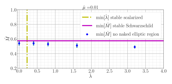
(a)

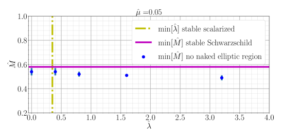
(b)

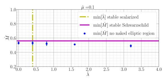
(c)

Figure 1: Onset of elliptic region formation, from evolution of perturbed Schwarzschild initial data as described in Sec. 6.1. The blue dots are our numerically computed values of $\hat{M}$, Eq. 3dghjkla, (for a given $\hat{\lambda}$, Eq. 3dghjkld) below which an elliptic region eventually forms outside the horizon. The error bars about each point come from truncation error estimates, computed by taking the difference of the elliptic onset point computed with two different resolutions: $N_{x}=2^{10}+1$ and $N_{x}=2^{11}+1$ radial points. The solid purple horizon line is the minimum $\hat{M}$ for a stable Schwarzschild black hole, and the dash-dotted yellow vertical line is the minimum $\hat{\lambda}$ for a stable scalarized black hole, with respect to linear radial perturbations according to the analysis of [1].

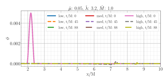
(a) Scalar field disperses

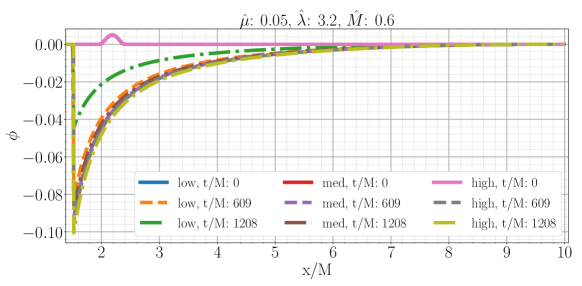
(b) Scalarized black hole forms

(c) Elliptic region formation

Figure 2: Example evolution for EdGB solution with compact scalar field initial data as described in Sec. 6.1. Regarding the scalarized black hole case (b), there is some truncation error induced decay of the scalar field at late times, most evident in the lower resolution case (dash-dot green curve), however with increasing resolution we do find convergence to a stable, static scalarized black hole. Low resolution for cases (a) and (c) is $N_{x}=2^{10}+1$ grid points, and for case (b) $N_{x}=2^{9}+1$ grid points. In all cases med and high resolution are double and quadruple the low resolution respectively.

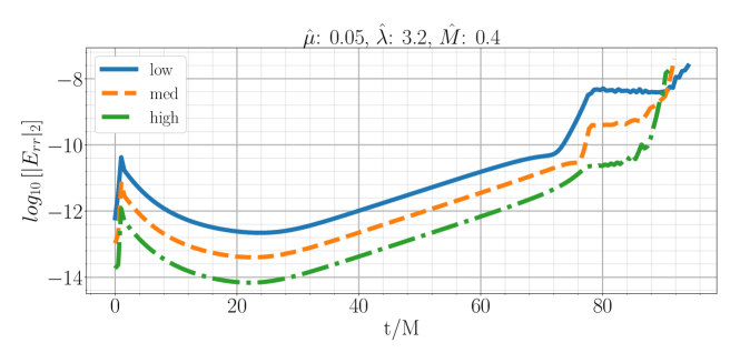
Figure 3: Two-norm of the independent residual $E_{rr}$ for a run that forms a naked elliptic region, with compact scalar initial data (see lower panel of Fig. 2). We see convergence up until near the formation of the elliptic region. Low resolution corresponds to $N_{x}=2^{10}+1$ grid points, and med and high resolution correspond to double and quadruple that number of grid points. See Sec. 6.1 for simulation parameters.

6.2 Numerical results: approximately scalarized black hole initial data

The results of evolving the approximate scalarized initial data described in Sec. 5.3 are qualitatively similar to that of the perturbed Schwarzschild case described in the previous section; Fig. 4 is the analogous plot to that of Fig.1 to illustrate. For the relevant initial data parameter we chose $\Phi_{0}=0.05$ and $M=10$ in Eq. 3dghjkltv. We found empirically that choosing $\Phi_{0}=0.05$ provided a scalarized profile reasonably close to the final stable scalarized profiles for the $\hat{M}$, $\hat{\mu}$, and we considered (for the definition of $\hat{M}$, $\hat{\mu}$, and $\hat{\lambda}$ see respectively Eq. 3dghjkla, Eq. 3dghjklc, and Eq. 3dghjkld). See Fig. 5 for an example of evolution of this initial data to a stable scalarized profile.

We also note that the onset of elliptic region formation in this parameter space does appear to depend on the initial data as well. Comparing Fig. 1 and Fig. 4 we see that our results support the conclusion that an elliptic region may form at a larger value of $\hat{M}$ when we start with approximately scalarized initial data.

(a)

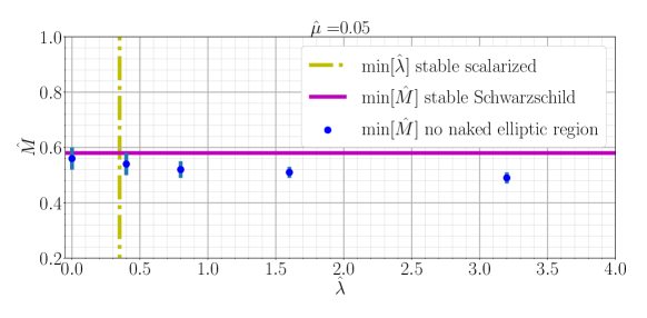
(b)

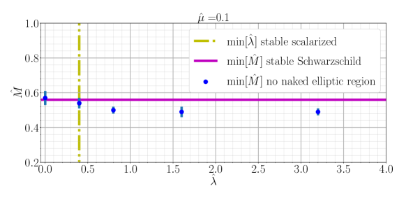
(c)

Figure 4: Onset of elliptic region formation, from evolution of approximate scalarized black hole initial data as described in Sec. 6.2. This is the analog of Fig. 1, and the same caption applies here. For definitions of $\hat{M}$ and $\hat{\lambda}$ see respectively Eq. 3dghjkla and Eq. 3dghjkld.

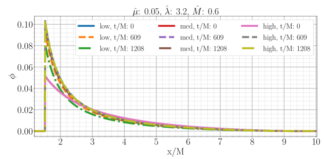
Figure 5: Formation of stable scalarized black hole from approximate scalarized initial data as described in Sec. 6.2. We show runs with three different resolutions: ‘low’, ‘med’, and ‘high’; ‘low’ resolution corresponds to $N_{x}=2^{10}+1$ radial grid points and ‘med’ and ‘high’ correspond to double and quadruple this number of radial points.

7 Discussion

We have numerically investigated perturbed black hole solutions in a $\mathbb{Z}_{2}$ symmetric (i.e. a theory with an action invariant under the operation $\phi\to-\phi$) variant of EdGB gravity. We have found, consistent with the linear analysis of [1], that stable scalarized black holes exist within this theory. However, for sufficiently large couplings relative to the scale of the black hole the theory dynamically loses hyperbolicity: the scalar field grows around the black hole until an elliptic region expands past the black hole horizon. These results, along with the recent results of [6, 7], suggests that in a limited parameter range scalarized black holes are subject to well-posed hyperbolic evolution. It would be interesting to see whether this conclusion extends beyond spherical symmetry, for example for binary black hole inspiral and merger. The existence of naked elliptic regions in the theory for sufficiently large couplings though strongly suggests that the theory makes most sense from an effective field theory point of view (which was the original motivation for the particular form of EdGB gravity studied here[1]).

The code[24] we wrote and used to produce the simulation results presented here can easily be altered to accommodate other forms of Gauss-Bonnet coupling $W(\phi)$ and scalar field potential $V(\phi)$. It would be interesting to investigate how these potential functions influence the structure of scalarized black holes that can form, and the region of solution space hampered by naked elliptic regions. It would also be interesting to include the $(\nabla\phi)^{4}$ term in action, to see the full range of dynamics that could occur for this class of $\mathbb{Z}_{2}$ symmetric scalar-tensor theories.

Appendix A Characteristics versus linearized perturbation analysis

Here we provide a brief discussion of the difference between linear perturbation theory analysis to identify stable/unstable modes (which is what is done in [1]) and characteristic analysis (which is the analysis we perform in our code).

The scalar field offers the only dynamical degree of freedom in EdGB gravity in spherical symmetry. The authors in [1] linearized the dynamics of that degree of freedom (which we denote by $\varphi$), and found that for a static background it obeys an equation of the form

$$h(r)\frac{\partial^{2}\varphi}{\partial t^{2}}-\frac{\partial^{2}\varphi}{\partial r^{2}}+k(r)\frac{\partial\varphi}{\partial r}+p(r)\varphi=0,$$ (3dghjklty)

where $h,k,p$ are functions of the static background geometry. They considered solutions of the form $\varphi(t,r)=e^{i\omega t}\psi(r)$, and searched for conditions that would make $\omega^{2}<0$.

The characteristics of Eq. 3dghjklty are found by keeping only highest derivative terms and replacing $\partial_{t}\to\xi_{t}$, $\partial_{r}\to\xi_{r}$, where $\xi_{a}\equiv(\xi_{t},\xi_{r})$ is the characteristic vector (see e.g. [28, 29], or[10, 12] in the context of shift symmetric EdGB gravity), and finding the zeros of this principal symbol of the system:

$$h(r)\xi_{t}^{2}-\xi_{r}^{2}=0.$$ (3dghjkltz)

The solutions $c\equiv-\xi_{t}/\xi_{r}$ to this equation give the radial characteristic speeds. Finding $\omega^{2}<0$ solutions to Eq. 3dghjklty can simply indicate a particular background solution is unstable to perturbations. In that case, as long as the theory remains hyperbolic the unstable solution could evolve to a different, stable one. By contrast, finding a $c^{2}<0$ solution to Eq. 3dghjkltz indicates a breakdown of hyperbolicity of the theory evaluated at that solution. When hyperbolicity has broken down, the equations of motion can no longer be solved as evolution equations.

We emphasize that the form of the characteristic equation we solve, Eq. 3dghjklo, does not take the form Eq. 3dghjkltz, as we solve the characteristic equation within a dynamical spacetime, and we use a different coordinate system than is used in [1]. Instead the characteristic equation takes the schematic form (compare to Eq. 3dghjklp)

$$\mathcal{A}\xi_{t}^{2}-\mathcal{B}\xi_{t}\xi_{r}+\mathcal{C}\xi_{r}^{2}=0,$$ (3dghjkltaa)

where $\mathcal{A}$, $\mathcal{B}$, and $\mathcal{C}$ depend on the background fields $\alpha$, $\zeta$, $P$, $Q$, and their radial and time derivatives.

From the forms of Eq. 3dghjklty and Eq. 3dghjkltz it is clear that linear (in)stability does not necessarily imply (lack of) hyperbolicity, or vice-versa. Nevertheless our hyperbolicity analysis does conform with the general results of [1].

Appendix B Approximate scalarized profile

Here we provide a derivation of the approximate scalarized black hole initial data presented in Sec. 5.3.

Consider a Schwarzschild background: we set $\alpha=1$, $\zeta=\sqrt{2m/r}$, set $\partial_{t}\phi=0$, and solve Eq. 3b

$$\nabla_{\mu}\nabla^{\mu}\phi-\left(\mu^{2}-\frac{1}{4}\eta\mathcal{G}\right)\phi-4\lambda\phi^{3}=0.$$ (3dghjkltab)

Plugging things in, we find

$$\left(1-\frac{2m}{r}\right)\frac{d^{2}\phi}{dr^{2}}+2\left(1-\frac{m}{r}\right)\frac{1}{r}\frac{d\phi}{dr}-\left(\mu^{2}-\frac{12\eta m^{2}}{r^{6}}\right)\phi-4\lambda\phi^{3}=0.$$ (3dghjkltac)

In the far field limit $(r\to\infty)$, and assuming $\lim_{r\to\infty}\phi=0$, we have to leading order

$$\frac{d^{2}\phi}{dr^{2}}+\frac{2}{r}\frac{d\phi}{dr}=\mu^{2}\phi.$$ (3dghjkltad)

The solution consistent with the field going to zero at spatial infinity is

$$\phi(r)=\frac{C}{r}\mathrm{exp}\left(-\mu r\right),$$ (3dghjkltae)

where $C$ is a constant. We can split up this constant into two as follows:

$$\phi(r)=\frac{c_{1}}{r}\mathrm{exp}\left(-\mu(r-c_{2})\right).$$ (3dghjkltaf)

In our simulations we set $c_{2}=3m$ on the initial data slice, see Eq. 3dghjkltv.

References

References

- [1] Macedo C F B, Sakstein J, Berti E, Gualtieri L, Silva H O and Sotiriou T P 2019 Phys. Rev. D99 104041 (Preprint 1903.06784)
- [2] Abbott B P et al. (Virgo, LIGO Scientific) 2016 Phys. Rev. Lett. 116 221101 (Preprint 1602.03841)
- [3] Yunes N, Yagi K and Pretorius F 2016 Phys. Rev. D94 084002 (Preprint 1603.08955)
- [4] Okounkova M, Stein L C, Scheel M A and Hemberger D A 2017 Phys. Rev. D96 044020 (Preprint 1705.07924)
- [5] Okounkova M, Scheel M A and Teukolsky S A 2019 Phys. Rev. D99 044019 (Preprint 1811.10713)
- [6] Kovacs A D and Reall H S 2020 (Preprint 2003.08398)
- [7] Kovacs A D and Reall H S 2020 (Preprint 2003.04327)
- [8] Misner C W, Thorne K S and Wheeler J A 1973 Gravitation (San Francisco: W. H. Freeman) ISBN 9780716703440
- [9] Nakahara M 2018 Geometry, Topology and Physics (Boca Raton, FL, USA: Francis & Taylor Group) ISBN 9781420056945 URL https://books.google.com/books?id=p2C1DwAAQBAJ
- [10] Ripley J L and Pretorius F 2019 Phys. Rev. D99 084014 (Preprint 1902.01468)
- [11] Ripley J L and Pretorius F 2020 Phys. Rev. D101 044015 (Preprint 1911.11027)
- [12] Ripley J L and Pretorius F 2019 Class. Quant. Grav. 36 134001 (Preprint 1903.07543)
- [13] Silva H O, Sakstein J, Gualtieri L, Sotiriou T P and Berti E 2018 Phys. Rev. Lett. 120 131104 (Preprint 1711.02080)
- [14] Adler R J, Bjorken J D, Chen P and Liu J S 2005 Am. J. Phys. 73 1148–1159 (Preprint gr-qc/0502040)
- [15] Ziprick J and Kunstatter G 2009 Phys. Rev. D 79(10) 101503 (Preprint 0812.0993) URL https://link.aps.org/doi/10.1103/PhysRevD.79.101503
- [16] Kanai Y, Siino M and Hosoya A 2011 Prog. Theor. Phys. 125 1053–1065 (Preprint 1008.0470)
- [17] Ripley J L 2019 Class. Quant. Grav. 36 237001 (Preprint 1908.04234)
- [18] Blázquez-Salcedo J L, Doneva D D, Kunz J and Yazadjiev S S 2018 Phys. Rev. D98 084011 (Preprint 1805.05755)
- [19] Minamitsuji M and Ikeda T 2019 Phys. Rev. D 99(4) 044017 URL https://link.aps.org/doi/10.1103/PhysRevD.99.044017
- [20] Silva H O, Macedo C F B, Sotiriou T P, Gualtieri L, Sakstein J and Berti E 2019 Phys. Rev. D 99(6) 064011 URL https://link.aps.org/doi/10.1103/PhysRevD.99.064011
- [21] Doneva D D and Yazadjiev S S 2018 Phys. Rev. Lett. 120(13) 131103 URL https://link.aps.org/doi/10.1103/PhysRevLett.120.131103
- [22] Press W H, Teukolsky S A, Vetterling W T and Flannery B P 2007 Numerical Recipes 3rd Edition: The Art of Scientific Computing 3rd ed (USA: Cambridge University Press) ISBN 0521880688
- [23] Gustafsson B, Kreiss H and Oliger J 1995 Time Dependent Problems and Difference Methods A Wiley-Interscience Publication (Wiley) ISBN 9780471507345 URL https://books.google.com/books?id=1JZ2mSQ-O6MC
- [24] Ripley J 2020 JLRipley314/spherically-symmetric-Z2-edgb: Spherically symmetric Z2 symmetric EdGB gravity, v1 URL https://doi.org/10.5281/zenodo.3873503
- [25] Thornburg J 2007 Living Reviews in Relativity 10 3 ISSN 1433-8351 URL https://doi.org/10.12942/lrr-2007-3
- [26] Sotiriou T P 2015 Class. Quant. Grav. 32 214002 (Preprint 1505.00248)
- [27] Berti E, Cardoso V and Starinets A O 2009 Class. Quant. Grav. 26 163001 (Preprint 0905.2975)
- [28] Lax P 1973 Hyperbolic Systems of Conservation Laws and the Mathematical Theory of Shock Waves (CBMS-NSF Regional Conference Series in Applied Mathematics no nos. 11-16) (Society for Industrial and Applied Mathematics) ISBN 9780898711776 URL https://books.google.com/books?id=L1vTdBhlSTMC
- [29] Kreiss H and Lorenz J 1989 Initial-boundary Value Problems and the Navier-Stokes Equations v. 136 (Academic Press) ISBN 9780124261259 URL https://books.google.com/books?id=3qEdlQEACAAJ