Simple Analytic Models of Gravitational Collapse

Abstract

Most general relativity textbooks devote considerable space to the simplest example of a black hole containing a singularity, the Schwarzschild geometry. However only a few discuss the dynamical process of gravitational collapse, by which black holes and singularities form. We present here two types of analytic models for this process, which we believe are the simplest available; the first involves collapsing spherical shells of light, analyzed mainly in Eddington-Finkelstein coordinates; the second involves collapsing spheres filled with a perfect fluid, analyzed mainly in Painleve-Gullstrand coordinates. Our main goal is pedagogical simplicity and algebraic completeness, but we also present some results that we believe are new, such as the collapse of a light shell in Kruskal-Szekeres coordinates.

I Introduction

Black holes and singularities are certainly some of the most peculiar and interesting features of general relativityDavies . From the perspective of fundamental theory their properties are far from completely understood, especially their relation to quantum theoryFraser ; from the perspective of astrophysics and observational astronomy they seem more and more to play a central role in the physics of objects ranging from stellar to cosmological sizeMisner-Thorne-Wheeler .

Most general relativity textbooks devote considerable space to discussing the simplest example of a black hole containing a singularity, the Schwarzschild geometryMisner-Thorne-Wheeler ; Adler ; Landau ; Ohanian ; Kenyon ; Weinberg ; Rindler ; Schutz ; Wald ; D'Inverno , and some also discuss Kerr’s generalization to a rotating system, although only a few derive itAdler ; Schiffer . Most also explain, at least qualitatively, why black holes should exist in the real world, based on the instability of neutron stars of more than about 4 solar masses; even neutron degeneracy pressure is not sufficient to provide stability. A few texts also discuss Schwarzschild’s interior solution for a constant density starAdler ; Weinberg , which clearly illustrates some of the same instability features as more realistic neutron star models. But the actual dynamical process of collapse, whereby a massive body becomes a black hole, is a more complex dynamical problem, and is often either neglected or treated heuristically and qualitatively.

For a brief history of gravitational collapse see referenceHillman . The study of gravitational collapse dynamics began with the classic seminal work of Oppenheimer and SnyderOpenheimer , who set up the equations and gave a semi-quantitative discussion of the collapse of a spherical non-radiating star. They also found a complete analytic solution for the case of a uniform perfect fluid of zero pressure - now widely referred to as ”dust.” This example is less artificial than it might appear since the effect of pressure in a more realistic treatment turns out to be not very critical; but the treatment by Oppenheimer and Snyder involves some awkward algebra in its treatment of the boundary between the interior and exterior of the dust star.

Some textbooks discuss collapse much like Oppenheimer and Snyder, notably Landau and LifshitzLandau and Misner Thorne and WheelerMisner-Thorne-Wheeler . In particular these texts use a Novikov type coordinate system, in which the dust is co-moving in a bound orbitNovikov . This coordinate system is synchronous and co-moving, and is wonderfully simple conceptually, but almost equally awful algebraically. Due to the algebraic difficulty, we believe, this is not the simplest way to treat the problem. Most other texts give a heuristic but convincing analysis by comparing the motion of a dust particle just outside a collapsing dust sphere with the motion of the surface; matching this motion is equivalent to matching the exterior and interior geometries, which is a rather obvious but important theoremHarrison .

What we have tried to do in the present paper is to analyze dynamical collapse in as simple a way as possible by our choice of coordinates; we use Eddington-FinkelsteinEddington ; Finkelstein type coordinates for infalling incoherent light or ”null dust,” and Painleve-GullstrandPainleve ; Gullstrand type coordinates for perfect fluids, including dust. These coordinates seem almost magically well suited to this purpose, as we hope will become apparent in sections 2 and 5. We use zero energy fluid systems in contrast to negative energy bound systems as used in references [3] and [5], largely because the algebra is much simplerAdler . This choice seems to us well justified because the zero and nonzero energy systems have the same qualitative behavior as they approach the black hole state as seen from outside in terms of standard Schwarzschild time, and have exactly the same behavior as they approach the singularity as seen in terms of the proper time of a falling observer. Moreover the zero energy case does not have the awkward conceptual problem of the motion before the maximum size is reached, since the maximum size occurs at an infinite time in the past. We therefore believe the zero energy case is more illustrative and economical of effort.

Almost needless to say we have treated only spherically symmetric collapsing systems. The Birkhoff theorem guarantees that a spherically symmetric system does not emit gravitational radiation; non-spherically symmetric collapse generally entails gravitational radiation, making the problem vastly more complex, though also more interesting.

To achieve our goal of simple textbook type examples of collapse, we must pay a price, which is some degree of artificiality. The main artificiality is the spherical symmetry; also the in-falling shells of light or other massless material of sections 2 and 3 are not likely to be found in nature; similarly we do not expect to find the perfect fluid sphere surrounded by an elastic shell of section 5, or the zero pressure perfect fluid of sections 6 and 7.

Since our purpose in the present paper is overtly pedagogical, much of what we obtain here is known and available somewhere in the vast research literature, although obtained with different techniques and different coordinates. However we believe our treatment is the simplest, both conceptually and algebraically, mainly due to our coordinate choice. We do not know of any use of Painleve-Gullstrand coordinates in the present context, although they are becoming more widely usedParikh-Wilczek ; Parikh ; as will be seen in section 6 these coordinates combine a Schwarzschild type radial coordinate and a Friedmann-Robertson-Walker (FRW) type cosmological time coordinate to give a natural interpolating system for describing both the interior and exterior of a fluid sphere. While the Eddington-Finkelstein and Painleve-Gullstrand coordinates serve their mathematical purpose quite well, they have a number of drawbacks such as a “time” marker that is not well-behaved everywhere in spacetime, and they are not synchronous; we have therefore also treated the collapse of a thin shell of light by transforming to Kruskal-Szekeres coordinates, which are conformally flat and thus display the causal structure of the collapse process quite clearlyKruskal ; Szekeres . In Kruskal-Szekeres coordinates one has a nice picture for distinguishing real world black holes from ”eternal” black holes, with their associated wormholes and white hole segments, none of which may be expected to actually exist in our universe.

We use throughout this paper a rather novel technique for handling the boundary conditions between the fluid and the exterior, which we believe is physically clear.

Since the pioneering work of Oppenheimer and Snyder there has been an enormous amount of work on gravitational collapse and related topics, most directed to research rather than pedagogy. The present pedagogical paper originated from several research problems, one involving a formation mechanism for singularity-free black holes filled with heavy vacuum, and another involving a finite version of the standard or “concordance” cosmological model. For these we needed analytic collapse models that were algebraically simpler and more explicit than we found in the literature. Our hope is that our methods and models might also be of use to students and teachers in illustrating more standard gravitational collapse.

This paper is organized as follows: the first part (sections 2 to 4) deals with collapsing shells of incoherent light or null dust, which is entirely characterized by its null 4-velocity and energy density; the second part (sections 6 and 7) deals with spheres of perfect fluid, including some with nonzero pressure and some with non-uniform density. In section 2 we use Eddington-Finkelstein coordinates to obtain the metric for the collapse of a thin light shell onto a black hole to form a larger black hole, and the collapse of a thin light shell to form a black hole ab initio. The ab initio collapse is amusing in that it is almost certainly the simplest complete scenario for the formation of a black hole, albeit it a rather artificial one. In section 3 we use the results of section 2 to obtain the metric for the collapse of a thick shell of light, layer by layer. The density profile of the shell is largely arbitrary, and we give one specific example. In section 4 we transform the metric for the thin light shell collapse to conformably flat Kruskal-Szekeres coordinates in order to display the causal structure of the geometry in a clear way - nearly equivalent to a Penrose diagram; as already noted we use these coordinates to emphasize the difference between black holes formed by collapse and eternal Schwarzschild black holes. In section 5 we present our way of doing the classic problem of collapse of a uniform fluid sphere, using Painleve-Gullstrand coordinates for maximum simplicity. We also obtain an explicit solution for a nonzero pressure fluid with a linear equation of state: $p=\alpha\rho$; to balance the pressure gradient force at the surface we use the artifice of a thin elastic shell with tangential pressure instead of the slowly decreasing radial pressure of a real stellar system; our model is essentially a balloon with uniform internal density and pressure. The stress energy tensor of the surface is described by the radius of the sphere, its energy density, and the parameter $\alpha$; for $\alpha=0$ we recover the standard results for the dust ball. In section 6 we deal with zero pressure non-uniform dust spheres, with the density characterized by a largely arbitrary function; again using Painleve-Gullstrand coordinates we build up the system layer by layer, to obtain the standard results of Oppenheimer and Snyder and Landau and Lifshitz etc. We do not allow the dust layers to cross, which could give rise to infinite densities and superficial singularitiesSingh . We give one specific example of the metric of a non-uniform sphere; the special case of uniform density agrees with the analysis of section 5. Since this paper is mainly pedagogical we have throughout sacrificed brevity and included considerable algebraic detail; only elementary mathematical methods are used.

It is worth mentioning that some simple and fairly obvious extensions of the present work can be made. First, by a reversal of time the collapse of light shells can be viewed as outgoing radiation, so we may easily obtain results like those of Vaidya for the geometry of a radiating bodyVaidya . Similarly the collapse of the perfect fluid can be time reversed to yield the metric for a black hole emitting matter, that is a type of white hole. Also it is straightforward to include a cosmological constant term in the equations to obtain the metric for a collapsing system in an exterior Schwarzschild de Sitter geometry; due to its somewhat more cumbersome algebra we have not included this in the present paper, and leave it as an exercise. (See referenceLake .) We will say more about further extensions and applications in section 8.

II Thin Light Shells

The motion of light in Schwarzschild geometry is algebraically awkward at and inside the Schwarzschild radius when Schwarzschild coordinates are used, but it becomes quite simple in Eddington-Finkelstein (EF) coordinates. In this section we use EF coordinates to study the motion of light, the growth of a black hole by absorption of light, and the ab initio formation of a black hole by a thin shell of light. The last process is most likely the simplest model for the formation of a black hole by gravitational collapse.

The Schwarzschild metric in Schwarzschild coordinates is, with $c=1$,

$$ds^{2}=(1+u)dt_{s}^{2}-\frac{dr^{2}}{1+u}-r^{2}d\Omega^{2},\quad$$ (1)

where $u=-R/r$ and $d\Omega^{2}=d\theta^{2}+\sin^{2}\theta d\phi^{2}$. The black hole surface is a sphere at the Schwarzschild radius (twice the geometric mass) $R=2m=2GM$. It is both an infinite redshift surface where $g_{00}=0$ and a null surface or one-way-membrane. In terms of the Schwarzschild time coordinate both light and particles take an infinite time to reach the black hole surface from the exterior. Specifically, for light falling radially from $r_{i}$

$$\Delta t_{s}=r_{i}-r+R\ln\Big{(}\frac{r_{i}-R}{r-R}\Big{)}.$$ (2)

Thus light never reaches the surface but approaches asymptotically with a characteristic time $R$. It is for this reason that we introduce the EF time coordinate, in terms of which the surface is reached in a finite time. The EF time coordinate is obtained from the Schwarzschild time by a radially dependent shift

$$t_{s}=t+g(r).$$ (3)

This leads to the EF form of metric,

$$ds^{2}=dt^{2}-dr^{2}-r^{2}d\Omega^{2}+u(dt\pm dr)^{2},$$ (4)

provided that we choose the transformation function $g$ to obey

$$\frac{dg}{dr}=\pm\frac{u}{1+u}.$$ (5)

The solution to this is

$$g=\mp R\ln\Big{(}\frac{r}{R}-1\Big{)},$$ (6)

which has an infinite stretch at $r=R$. Henceforth we refer to the coordinates and metric form in Eq.(4) as EF for any function $u(r,t)$.

The EF form is extremely convenient because radially infalling light behaves quite simply if the plus sign in Eq.(4) is chosen. For such light we set the line element equal to zero, to obtain

$$ds^{2} = dt^{2}-dr^{2}+u(dt+dr)^{2}$$ (7)

$$= (dt+dr)(dt-dr+udt+udr)=0.$$

so that

$$dt+dr=0,\quad t+r={\rm const}, \quad\textrm{infalling light},$$ (8)

$$dr/dt=(1+u)/(1-u), \quad\textrm{outgoing light}.$$ (9)

Thus the path of infalling light is independent of the metric function $u$, and is the same as in flat space. See Fig. 1. Conversely, outgoing light “stalls” where $u=-1$ and $g_{00}=0$, that is at the infinite redshift surface.

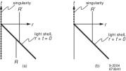
Figure 1: In (a) a thin light shell falls into a black hole to produce a larger black hole. In (b) a thin light shell with flat Minkowski interior collapses to form a black hole.

We will soon need the Einstein tensor for the EF metric form Eq.(4). Its nonzero components are easily calculated to be

$$G^{0}_{\;0}=\frac{u^{\prime}}{r}+\frac{u}{r^{2}},\quad G^{1}_{\;0}=-\frac{\dot{u}}{r},\quad G^{0}_{\;1}=\frac{\dot{u}}{r},$$

$$G^{1}_{\;1}=\frac{u^{\prime}}{r}+\frac{u}{r^{2}}-\frac{2\dot{u}}{r},$$

$$G^{2}_{\;2}=G^{3}_{\;3}=\frac{u^{\prime}-\dot{u}}{r}+\frac{\ddot{u}+u^{\prime\prime}-2\dot{u}^{\prime}}{2}.$$ (10)

Here a dot denotes a time derivative and a prime denotes a radial derivative. We define the stress energy tensor in terms of the Einstein tensor by using the field equations

$$G^{\alpha}_{\;\beta}\equiv-8\pi GT^{\alpha}_{\;\beta}.$$ (11)

For pure Schwarzschild geometry the Einstein tensor is everywhere zero, as is easily verified.

We now study the formation of a black hole by a single thin shell of light, and in the next section we will consider a thick shell of light. For both purposes we begin with a thin shell of light falling into a Schwarzschild black hole with radius $R$ to form a black hole with radius $R^{\prime}$ as shown in Fig. 1a; the light shell obeys $r+t=0$ everywhere. We may write the metric in all of spacetime using a step function $\Theta$ and its complement $\tilde{\Theta}=1-\Theta$ , as

$$u=-\frac{R}{r}\tilde{\Theta}(r+t)-\frac{R^{\prime}}{r}\Theta(r+t),$$ (12)

which is of course time dependent. Substituting this into Eq.(62) and Eq.(11) we obtain the stress-energy tensor for the thin light shell, which is singular due to the step function,

$$T^{\alpha}_{\;\beta}=\frac{R^{\prime}-R}{8\pi Gr^{2}}\delta(r+t)k^{\alpha}k_{\beta},\quad$$ (13)

where $k^{\alpha}=(1,-1,0,0)$ and $k_{\beta}=(1,1,0,0)$. The null vector $k^{\alpha}$ corresponds to infalling light. From the energy density $T^{0}_{\;0}$ we may calculate the energy or effective mass of the light shell by going to a time in the distant past when the shell was in asymptotically flat space,

$$M_{s}=\int 4\pi r^{2}T^{0}_{\;0}dr=\frac{R^{\prime}-R}{2G}=M^{\prime}-M.$$ (14)

This verifies that the mass of the initial black hole plus the energy or effective mass of the light shell equals the mass of the final black hole.

The above results hold for the special case when the initial black hole is replaced by flat space, or $R=0$. Note that everything above is consistent with the interior of a spherical thin light shell being flat Minkowski space. This represents the formation of a black hole by the gravitational collapse of a single thin light shell (or other massless material), as shown in figure 1b; this would seem to be the simplest complete example of gravitational collapse.

III Thick Light Shells

Our results from the preceding section may be used to construct a model for the collapse of a thick light shell, layer by layer. The initial state is a sequence of concentric thin shells with a flat Minkowski interior, as shown in Fig. 2a. Each region of spacetime has a Schwarzschild geometry as discussed in the previous section. The innermost shell with energy $\Delta m_{1}$ collapses to form a black hole of mass $m_{1}=\Delta m_{1}$, followed by others to form intermediate black holes of mass $m_{j}=\Delta m_{1}+\cdots+\Delta m_{j}$, ending with a final black hole with mass $m_{f}$ and Schwarzschild radius $R=2m_{f}$. Between the shells the geometry is given by Eq.(4), with a metric function

$$u=-2m_{j}/r.$$ (15)

The evolving infinite redshift surface, defined by $u=-1$, is the zigzag line in Fig. 2a.

The continuous analog of the sequence is a family of concentric shells with a continuous label $\lambda$, which we choose to run from 0 to 1. The parameter $\lambda$ plays the same role as the discrete label $j$: that is the energy or effective mass inside the $\lambda$ shell is denoted by $m(\lambda)$. As in Eq.(15) the metric function in the light shell is

$$u=-2m(\lambda)/r.$$ (16)

The evolving infinite redshift surface is the smooth line in Fig. 2b.

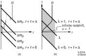
Figure 2: In (a) a discrete sequence of light shells forms a black hole; (b) shows the continuous version of the same process.

A labeling scheme, which is convenient for both the present light shell and the fluid systems to be discussed later, is to take the energy inside the $\lambda$ shell to be proportional to $\lambda$,

$$m(\lambda)=\lambda m_{f},\quad m_{f}=\textrm{final mass}.$$ (17)

The time at which the $\lambda$ shell reaches the center may be chosen almost arbitrarily as a function of $\lambda$, subject to the constraints that it be 0 for the innermost shell $\lambda=0$ and increase monotonically to the final time $\Delta$ for the outermost shell $\lambda=1$, as shown in Fig. 2. We denote this function as $F^{-1}(\lambda)\Delta$, for reasons that will become apparent. The equation of motion for the shell $\lambda$ is thus

$$r+t=F^{-1}(\lambda)\Delta.$$ (18)

From its definition $F^{-1}$ must have an inverse, so we may invert this to obtain

$$\lambda=F\Big{(}\frac{r+t}{\Delta}\Big{)},\quad m(\lambda)=m_{f}\lambda=m_{f}F,$$ (19)

with $F(0)=0$ and $F(1)=1$. Thus $F$ serves as a density profile function, and the metric in the interior of the light shell may be written as

$$u=-\frac{2m_{f}}{r}F\Big{(}\frac{r+t}{\Delta}\Big{)}=-\frac{RF}{r}.$$ (20)

The infinite redshift surface, defined by $u=-1$, is thus determined by

$$r=R\,F\Big{(}\frac{r+t}{\Delta}\Big{)}.$$ (21)

Inverting this we obtain for the infinite redshift surface

$$t=\Delta F^{-1}(r/R)-r.$$ (22)

This implies that if the total duration of collapse $\Delta$ is sufficiently large then $t$ must be a positive monotonic function of $r$.

Using the metric function Eq.(20) we may calculate the Einstein tensor and the stress-energy tensor from Eq.(10) and Eq.(11). This gives for the light shell,

$$T^{\alpha}_{\;\beta}=\frac{RF^{\prime}}{8\pi Gr^{2}\Delta}k^{\alpha}k_{\beta},\quad\textrm{light shell},$$ (23)

where $F^{\prime}$ denotes the derivative of $F$ with respect to its argument, and $k^{\alpha}$ is the null vector defined in Eq.(13). From this we obtain the energy density and the total energy of the light shell as

$$\rho=T^{0}_{\;0}=\frac{RF^{\prime}}{8\pi Gr^{2}\Delta},$$

$$M_{s}=\int 4\pi r^{2}\rho dr=\frac{m_{f}F(1)}{G}=\frac{m_{f}}{G},$$ (24)

where the integral is again done in the asymptotically flat spacetime of the distant past, verifying that the energy of the light shell is equal to the final black hole mass.

Our approach to boundaries and boundary conditions is somewhat unorthodox; we do not impose boundary conditions per se on the metric function between regions of spacetime. Instead we use the above solutions (in vacuum and within the light shell) to calculate the stress-energy tensor, which is defined by the field equations and Eq.(10). The resulting stress energy tensor must be zero in vacuum, correctly represent the stress energy within the light shell, and describe the stress on the boundaries. If it does, the solution makes physical sense. For the region near the inner and outer boundaries of the light shell we may write the metric function as

$$u=\left\{\begin{array}[]{ll}-(RF/r)\Theta(r+t),&\textrm{inner surface},\\ -(RF/r)\tilde{\Theta}(r+t-\Delta),&\textrm{outer surface}.\end{array}\right.$$ (27)

Calculating the stress energy tensor from Eq.(10) and Eq.(11) we find that there is no singular shell at these boundaries since the relevant singular derivatives cancel; thus the stress-energy tensor associated with the boundaries is zero and the solution is thus physically reasonable.

As a specific example let us take the density profile function to be linear,

$$F\Big{(}\frac{r+t}{\Delta}\Big{)}=\frac{r+t}{\Delta},\quad m(\lambda)=m_{f}\Big{(}\frac{r+t}{\Delta}\Big{)}.$$ (28)

This corresponds to a constant rate of energy impacting the center. From Eq.(20) the metric function in the various regions is,

$$u=\left\{\begin{array}[]{ll}0,&\textrm{Minkowski region},\\ -R/r,&\textrm{Schwarzschild region},\\ -R(r+t)/(r\Delta),&\textrm{within light shell}.\end{array}\right.$$ (32)

The infinite redshift surface, from Eq.(21), is the linear function

$$t=\Big{(}\frac{\Delta}{R}-1\Big{)}r.$$ (33)

The slope of this is positive for $\Delta/R>1$, that is when the light shell thickness is greater than its Schwarzschild radius. Within the light shell the energy density is, from Eq.(10) and Eq.(11),

$$T^{0}_{\;0}=\rho=\frac{R}{8\pi Gr^{2}\Delta},\quad\textrm{light shell interior,}$$ (34)

which is independent of time.

In Fig. 3 we show a qualitative sketch of some outgoing light rays for a fairly general light shell. The sketch is made by noting that, from Eq.(9): the slope of outgoing rays is 1 in the Minkowski region and at large distances it approaches 1; the slope is 0 along the infinite redshift surface; finally, the slope is -1 at the center of the black hole. There is a last-ray-out emitted from the origin to infinity, after which all outgoing rays (as well as particles) are trapped within the surface at $R$ and eventually fall into the singularity. The surface defined by the last-ray-out is thus a global horizon. This illustrates that the horizon and the infinite redshift surface are quite different inside the time dependent light shell, unlike the situation for the time independent Schwarzschild geometry.

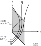
Figure 3: Some “outgoing” light rays in the thick light shell collapse. The last ray out (B) hovers at the Schwarzschild radius and defines a horizon.

As a further application of our methods we note that our results can be reversed in time to describe radiation being emitted by a spherically symmetric system such as a star or black hole Vaidya ; Hawking ; Gibbons ; Hawking-Penrose . To do this we use the minus sign for the metric in Eq.(4) and turn the diagram in Fig.2b upside down. It is then easy to modify our algebraic results to describe any reasonable light shell density profile. This may be useful in studying the final stages of black hole evaporation, when the gravitational field of the radiation becomes comparable to that of the black hole and cannot be neglected Parikh-Wilczek ; it might help in determining if a black hole radiates entirely away to vacuum or leaves behind a remnant Adler-Santiago ; Adler-Chen-Santiago .

IV Thin Light Shells in Kruskal-Szekeres Coordinates

The thin light shell discussed in section 2 is probably the simplest model of gravitational collapse. However in EF coordinates $g_{00}$ is negative for the interior of the black hole. This means that if one is at coordinate rest $(dr=d\theta=d\phi=0)$ then the square of the proper time interval $ds^{2}$ has the opposite sign of the square of the coordinate time interval $dt^{2}$, so that $t$ may not be interpreted as a good time marker in that region of spacetime. The same is true of Schwarzschild coordinates. Kruskal-Szekeres (KS) coordinates, which are discussed in many texts, were developed to solve this problemKruskal ; Szekeres ; Adler . Here we will obtain KS type coordinates for the thin light shell collapse of section 2.

By KS coordinates we mean a system in which the $t,r$ part of the metric is conformal to flat Minkowski space, with no singularities or zeroes. We first show how a metric in EF form, with $u=u(r)$, may be put into conformal form. The metric Eq.(4) may be factored as follows, with angular dependence suppressed,

$$ds^{2} = dt^{2}-dr^{2}+u(dt+dr)^{2}$$ (35)

$$= (1+u)(dt+dr)(dt-\frac{1-u}{1+u}dr)$$

$$= (1+u)d(t+r)d(t-\sigma),\quad\sigma\equiv\int\frac{1-u}{1+u}dr.$$

The quantities $t+r$ and $t-\sigma$ are termed conformal null coordinates since the line element is zero along lines of constant $t+r$ or $t-\sigma$; these thus represent radially moving light rays. We transform to other null conformal coordinates by choosing any functions $w(r+t)$ and $v(\sigma-t)$, so that

$$dw=w^{\prime}(r+t)d(r+t),\quad dv=v^{\prime}(\sigma-t)d(\sigma-t),$$ (36)

so the metric in terms of $w,v$ is

$$ds^{2}=-\frac{1+u}{w^{\prime}v^{\prime}}dwdv=Hdwdv.$$ (37)

The metric function $H$ may be considered to be a function of $r$ and $t$, or $w$ and $v$. We may also relate the null coordinates to Lorentz-like coordinates,

$$w=\tau+\rho,\quad v=\tau-\rho,\quad ds^{2}=H(d\tau^{2}-d\rho^{2}).$$ (38)

Thus $\tau$ and $\rho$ may be interpreted as time and radial coordinates provided that $H$ is positive and has no singularities or zeros.

Outside the Schwarzschild radius and the light shell the function $\sigma$ and a convenient choice for the functions $w$ and $v$ are the following

$$\sigma(r)=\int\frac{r+R}{r-R}dr=r+2R\ln\Big{(}\frac{r}{R}-1\Big{)},\quad r>R,$$

$$w_{s}=\gamma e^{a(t+r)},v_{s}=\omega e^{a(\sigma-t)}=\omega e^{a(r-t)}\Big{(}\frac{r}{R}-1\Big{)}^{2aR},$$

$$H_{s}=\frac{-1}{\gamma\omega a^{2}r}e^{-2ar}R^{2aR}(r-R)^{1-2aR},$$ (39)

where $a,\gamma,\omega={\rm const.}$ This transformation is chosen to make $H_{s}$ independent of time. In order that $H_{s}$ also be nonsingular and have no zeros we choose $a=1/2R$, and to map the exterior region to the $w_{s}>0,v_{s}<0$ quadrant we choose $\gamma=1$ and $w=-1$. Then the transformation and metric functions are explicitly

$$w_{s}=e^{\frac{r+t}{2R}},\quad v_{s}=e^{\frac{r-t}{2R}}\Big{(}1-\frac{r}{R}\Big{)},\quad H_{s}=\frac{4R^{3}}{r}e^{-\frac{r}{R}}.\quad$$ (40)

Note that $w_{s}$ and $v_{s}$ are dimensionless and $H_{s}$ is the square of a distance.

For the interior of the black hole, $r<R$, and outside the light shell (see Fig.1b) we choose the opposite sign for the logarithm and $\gamma=\omega=1$ in Eq.(39), to obtain the same expression as in Eq.(40), which is thus valid throughout the Schwarzschild geometry. The expressions Eq.(40) are similar to the standard ones used to transform between Schwarzschild coordinates and KS coordinates, but differ in important ways. Lines of $r=$const. map to hyperbolae with $w_{s}v_{s}={\rm const.}$; in particular $r=0$ corresponds to $w_{s}v_{s}=1$ and $r=R$ corresponds to $w_{s}v_{s}=0$. The lines $t=\infty$ and $r=R$ both map to $v_{s}=0$, while $t=-\infty$ maps to $w_{s}=0$. (Unlike the case with Schwarzschild coordinates lines of constant $t$ do not map to rays of $v_{s}/w_{s}={\rm const.}$!) See Fig. 4.

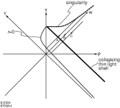
Figure 4: Collapse of a thin light shell in KS coordinates, to be compared with Fig. 1b in EF coordinates. Only the spacetime region to the right of the line $r=0$ has physical meaning. Compare the light rays A B C to those in Fig. 3.

There are many ways to transform from EF to KS coordinates for the Minkowski geometry inside the light shell; of course Minkowski geometry in EF coordinates is already in KS form, but not one that is useful to us. We must choose a transformation that joins continuously with the transformation Eq.(40) along the boundary line $r+t=0$, and we also demand that the function $H$ be continuous along that line. For that space the metric function $u=0$, so that from Eq.(35) $\sigma=r$. Thus from Eq.(37) the metric function $H$ is

$$H_{m}=\frac{-1}{w^{\prime}_{m}(r+t)v^{\prime}_{m}(r-t)}.$$ (41)

Equating this with $H_{s}$ from Eq.(40) along $r+t=0$ we obtain a differential equation for $v_{m}$

$$v^{\prime}_{m}(2r)=\frac{-1}{4R^{3}w^{\prime}_{m}(0)}re^{r/R}.$$ (42)

That is, in terms of the argument, denoted $x$,

$$v^{\prime}_{m}(x)={\rm(const.)}xe^{x/2R},\quad$$

$$v_{m}(x)={\rm(const.)}(x-2R)e^{x/2R}.$$ (43)

For continuity we choose $w_{m}$ to be the same as in the Schwarzschild region Eq.(40), so with appropriate constants we arrive at

$$w_{m}=e^{\frac{r+t}{2R}},$$

$$v_{m}=(1-\frac{r-t}{2R})e^{\frac{r-t}{2R}},$$

$$H_{m}=4R^{3}(\frac{2}{r-t})e^{-\frac{r}{R}}.\quad$$ (44)

These functions are obviously equal to those in Eq.(40) along the line $r+t=0$, as desired. Note that the price we pay for having $H_{s}$ in the Schwarzschild region independent of time is that $H_{m}$ in the Minkowski region is dependent on time.

The nature of the transformation Eq.(44) is best seen in terms of the mapping of some lines and points: $t=\infty$ maps to $v=0$; $t=-\infty$ maps to $w=0$; lines of constant $r+t$ map to constant $w$ lines; lines of constant $r-t$ map to constant $v$ lines; in particular $r+t=0$ maps to $w=1$ and $r=t=0$ maps to $w=v=1$. Finally the origin $r=0$ maps to

$$w_{m}=e^{t/2R},v_{m}=(1+\frac{t}{2R})e^{-t/2R},$$ (45)

so

$$v_{m}=\frac{1}{w_{m}}(1+\ln{w_{m}}).$$ (46)

Henceforth we drop the subscripts on $w$ and $v$.

Figure 4 show the complete collapse process, with the Schwarzschild and Minkowski geometries stitched together along the line $r+t=0$. Only the region to the right of the line corresponding to $r=0$ has physical meaning. It is evident from the figure that the line $v=0$ defines a horizon, and it is also apparent that the singularity at $r=0$ does not behave like a time independent spatial position. Note also that $\rho$ serves as a radial marker, even though regions of the spacetime have negative $\rho$.

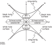
Figure 5: The pure or eternal Schwarzschild geometry in KS coordinates. The entire spacetime region shown is given physical meaning in terms of a white hole region and a second exterior Schwarzschild region. Compare to Fig. 4. See for example references [3,4].

Figure 4 may be compared with the ”pure” or eternal Schwarzschild geometry discussed in many textbooks Misner-Thorne-Wheeler ; Adler and shown in KS coordinates in Fig. 5; this shows the ”maximum analytic extension” of the Schwarzschild solution. The region $w<0,v<0$ is interpreted as a white hole, and is absent in figure 4; also absent is the region $w<0,v>0$, interpreted as the ”other side of the wormhole,” and part of the interior region $w>0,v<0$. This illustrates that if the formation of the black hole by gravitational collapse is taken into account then the much-discussed white hole and wormhole regions are not present; there is no reason to expect that such regions occur in nature, as emphasized by Wheeler and many others Harrison .

V Uniform Fluid Spheres

The spherical shells of light used in the preceding sections provide very simple models of gravitational collapse but are rather artificial and do not approximate anything we expect to find in nature. We now turn to a more realistic system, a sphere of uniform perfect fluid with a linear equation of state. This includes our approach to the special case of a dust ball, the original Openheimer and still a favored system for collapse studies Misner-Thorne-Wheeler ; Landau ; Weinberg . We believe our approach is the simplest available, because the Painleve-Gullstrand (PG) coordinate system is remarkably well suited to the task Painleve ; Gullstrand .

Some of the mathematical techniques we used for light shells, such as use of concentric layers and the handling of the boundary conditions, will also prove useful for fluid spheres.

The fluid collapse involves only two spacetime regions, the fluid interior, and the Schwarzschild exterior. A crucial step is to find a metric form (the PG form) which describes both regions simply, and in which the motion of the fluid is simple.

The spacetime geometry corresponding to a uniform fluid is well known from cosmology; it is described by the Friedmann-Robertson-Walker metric in co-moving coordinates, which covers all of spacetime from the big bang onwards [3,4]. For simplicity we consider the spatially flat case, that is $k=0$, for which the metric is

$$ds^{2}=dt^{2}-a(t)^{2}(dr_{c}^{2}+r_{c}^{2}d\Omega^{2}).$$ (47)

(This corresponds to zero energy collapsing system.) The co-moving radial coordinate $r_{c}$ is dimensionless, while the scale function $a(t)$ is a solution of the cosmological equations, with the dimension of a length. To describe a finite sphere we truncate the radial coordinate at some value. If the fluid has a linear equation of state, with pressure and density obeying $p=\alpha\rho$, then the scale function is a power of $t$, specifically

$$a(t)=At^{n},\quad A={\rm const.},\quad n=\frac{2}{3(\alpha+1)}.$$ (48)

In particular dust (or “cold matter”) has negligible pressure so $\alpha=0$ and $n=2/3$, while radiation (or “hot matter”) has $\alpha=1/3$ and $n=1/2$. This is the range of normal matter. In the cosmological scenario time runs from the big bang at $t=0$ to infinity, but in the collapse scenario it will run from negative infinity to $t=0$. That is, a very large fluid sphere in the far distant past collapses toward zero size at $t=0$.

To obtain the desired form for the metric inside the fluid we introduce a new radial coordinate,

$$r=a(t)r_{c},$$ (49)

which is not co-moving, to obtain the metric

$$ds^{2} = [1-(r\dot{a}/a)^{2}]dt^{2}+2(r\dot{a}/a)drdt-dr^{2}-r^{2}d\Omega^{2}$$

$$= [1-(nr/t)^{2}]dt^{2}+2(nr/t)drdt-dr^{2}-r^{2}d\Omega^{2}.$$

This contains the single metric function $nr/t$ and is distinctive in having a cross term and $g_{rr}=-1$. It has an infinite redshift surface where $g_{00}=0$, or $nr/t=\pm 1$. The minus sign is appropriate since we will deal with negative times.

The empty region exterior to the fluid is described by the Schwarzschild metric in Eq.(1), which we now write in the form

$$ds^{2}=(1-\psi^{2})dt_{s}^{2}-\frac{dr^{2}}{1-\psi^{2}}-r^{2}d\Omega^{2},\quad\psi=\pm\sqrt{\frac{R}{r}}.$$

To make this compatible with the metric in Eq.(LABEL:UniformFluidPG) in the fluid we choose a new time coordinate that makes $g_{rr}=-1$. Taking

$$t_{s}=t+g(r),$$ (52)

we find that

$$ds^{2}=(1-\psi^{2})dt^{2}\pm 2\psi drdt-dr^{2}-r^{2}d\Omega^{2},$$ (53)

provided that $g$ obeys

$$g^{\prime}=\pm\frac{\psi}{1-\psi^{2}}.$$ (54)

As expected this transformation involves an infinite time stretch at the Schwarzschild radius, where $\psi^{2}=1$. For the Schwarzschild region the solution to Eq.(54) is

$$g=\mp R\left(2\sqrt{\frac{r}{R}}+\ln{\frac{\sqrt{r}-\sqrt{R}}{\sqrt{r}-\sqrt{R}}}\right).$$ (55)

The metric Eq.(53) and the transformation Eq.(55) are those obtained by Painleve and Gullstrand Painleve ; Gullstrand . Both regions of spacetime are now described by the metric form Eq.(53), with $\psi$ allowed to be a function of both $r$ and $t$; specifically

$$\psi=\left\{\begin{array}[]{ll}nr/t,&\quad\textrm{fluid interior},\\ -\sqrt{R/r},&\quad\textrm{Schwarzschild exterior}.\end{array}\right.$$ (58)

We choose the positive signs in Eq.(54) and negative sign in Eq.(55) to correspond to collapse during negative time, and refer to the metric form and coordinates as generalized Painleve-Gullstrand or simply PG.

The PG metric has a remarkable property that is crucial to our analysis. The geodesic equations for radial motion of a particle in the metric eq(53) lead, after some algebra, to

$$0 = \frac{d^{2}t}{ds^{2}}+\psi^{\prime}\left[(\frac{dt}{ds})^{2}-1\right],\quad\quad\psi^{\prime}\equiv\frac{\partial\psi}{\partial r},$$

$$1 = (1-\psi^{2})(\frac{dt}{ds})^{2}+2\psi\frac{dt}{ds}\frac{dr}{ds}-(\frac{dr}{ds})^{2}.$$ (59)

One obvious solution to the first is

$$dt/ds=1,\quad t=s-s_{0}.$$ (60)

Thus coordinate time and proper time intervals are equal for such a freely falling particle, and this holds for any metric function $\psi$. The second equation in Eq.(59) now becomes quite simple

$$\frac{dr}{ds}=\frac{dr}{dt}=\psi.$$ (61)

In the Schwarzschild region this is the same as the classical Newtonian equation for a radially falling test particle of zero energy.

We will soon need the Einstein tensor and the stress-energy tensor. From the PG metric form it is straightforward and only slightly tedious to calculate these. The nonzero components of the Einstein tensor are

$$G^{0}_{\;0}=-\frac{2\psi\psi^{\prime}}{r}-\frac{\psi^{2}}{r^{2}},\quad G^{1}_{\;0}=\frac{2\psi\dot{\psi}}{r},$$

$$G^{1}_{\;1}=-\frac{2\psi\psi^{\prime}}{r}-\frac{\psi^{2}}{r^{2}}-\frac{2\dot{\psi}}{r},$$

$$G^{2}_{\;2}=G^{3}_{\;3}=-\frac{\dot{\psi}+2\psi\psi^{\prime}}{r}-\dot{\psi}^{\prime}-\psi\psi^{\prime\prime}-\psi^{\prime\,2}.$$ (62)

As before we define the stress-energy tensor via the field equations $G^{\alpha}_{\;\beta}=-8\pi GT^{\alpha}_{\;\beta}$; in particular the energy density is

$$\rho=T^{0}_{\;0} = \frac{1}{8\pi G}(\frac{2\psi\psi^{\prime}}{r}+\frac{\psi^{2}}{r^{2}})$$ (65)

$$= \left\{\begin{array}[]{cl}0,&\textrm{exterior,}\\ \frac{3n^{2}}{8\pi Gt^{2}},&\textrm{interior.}\end{array}\right.$$

Thus the density is uniform, as expected.

We now join the spacetime regions inside and outside the fluid by demanding that the metric function $\psi$ in Eq.(58) be continuous across the fluid surface boundary. This gives

$$r^{3/2}+\frac{\sqrt{R}}{n}t=0.$$ (66)

The geodesic equation for a zero energy falling particle in the Schwarzschild exterior region is

$$r^{3/2}+\frac{3\sqrt{R}}{2}(t-t_{0})=0.$$ (67)

This agrees with the motion of the surface Eq.(66) only for the case of $n=2/3$, that is dust. Thus a freely falling particle may hover at the falling surface of a dust ball, as it should. However, if the pressure is nonzero and $n<2/3$ then the surface will fall more rapidly. This is due the stress in the surface layer, as we will see. Figure 6 shows the collapse scenario in PG coordinates.

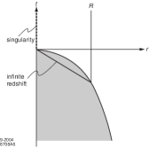
Figure 6: Collapse of a uniform fluid sphere to form a black hole in PG coordinates.

It is straightforward to calculate the stress-energy tensor for the fluid surface with the same technique we used in section 3. In the vicinity of the surface the metric function $\psi$ may be written

$$\psi=\frac{nr}{t}\tilde{\Theta}(r^{3/2}+\frac{\sqrt{R}}{n}t)-\sqrt{\frac{R}{r}}\Theta(r^{3/2}+\frac{\sqrt{R}}{n}t).$$ (68)

This leads to a singular stress-energy tensor

$$T^{2}_{\;2}=T^{3}_{\;3}=\frac{nr}{8\pi Gt^{2}}(1-\frac{3n}{2})\,\delta\left(r-(\sqrt{R}t/n)^{2/3}\right).$$ (69)

For a zero pressure fluid, $\alpha=0$ and $n=2/3$, this vanishes as expected. If the pressure is not zero it represents a surface tension, as we will now show. The surface tension of a fluid sphere is related to its radius and pressure by $\tau=pr/2$; in the present case this implies from Eq.(48) and Eq.(65),

$$\tau=\frac{pr}{2}=\frac{\alpha\rho r}{2}=\frac{nr}{8\pi Gt^{2}}(1-\frac{3n}{2}),$$ (70)

which agrees with Eq.(69). Thus the stress-energy tensor indeed represents a surface tension that balances the internal pressure of the fluid to keep it stable. This is why the surface falls faster than a freely falling particle.

In summary the collapse of a uniform fluid sphere is described by the metric function in Eq.(53) and Eq.(58), the density in Eq.(65), and the surface tension in Eq.(69). Its collapse is qualitatively similar to that of the light shells, but rather less artificial. Our use of surface tension to stabilize the surface is a conceptually simple substitute for the gradual pressure gradient of a more realistic model; such tangential pressures are also mentioned by Singh in Ref.[26] and in the references contained therein.

VI Zero Pressure Fluid Spheres

We next consider the collapse of a sphere filled with zero pressure perfect fluid, that is a dust ball. This problem is discussed by Landau and LifshitzLandau using Lemaitre-like coordinatesWeinstein . For simplicity and physical clarity we use the same technique as in section 3 for constructing thick light shells; that is we build the dust ball layer by layer from a sequence of thin dust shells. The layers are prohibited from crossing to prevent superficial singularities due to the consequent infinite densitySingh . PG coordinates will again be used, with the metric form Eq.(53) containing a single metric function $\psi(r,t)$. The Einstein tensor for this is given in Eq.(62), and we recall that in PG coordinates we may take proper time and coordinate time intervals to be equal along zero energy particle geodesics.

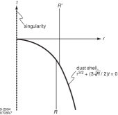
Figure 7: A thin shell of dust falls into a black hole to form a larger black hole in PG coordinates. This is the analog of Fig. 1 for light.

In analogy with section 3 we begin with a thin shell of dust falling onto a black hole, shown in Fig. 7. The shell is assumed to be very light, so that $m$ and $m^{\prime}$ differ by a small $\Delta m$, and the Schwarzschild radii differ by $2\Delta m$. As in Section 5 the metric function in the two Schwarzschild regions is

$$\psi=\left\{\begin{array}[]{ll}-\sqrt{R/r},&\textrm{initial Schwarzschild region},\\ -\sqrt{R^{\prime}/r},&\textrm{final Schwarzschild region}.\end{array}\right.$$ (73)

The equation of the thin dust shell is that of a geodesic for a zero energy particle in the Schwarzschild geometry, given in Eq.(67). It is important that coordinate and proper time intervals are equal along the geodesic, so that the equation for the boundary is a relation between the coordinates $r$ and $t$.

To obtain the stress-energy tensor for the dust shell we write the metric in the vicinity of the boundary as

$$\psi= - \sqrt{\frac{R}{r}}\tilde{\Theta}(\sqrt{r^{3}}+\frac{3}{2}\sqrt{R}t)$$ (74)

$$- \sqrt{\frac{R^{\prime}}{r}}\Theta(\sqrt{r^{3}}+\frac{3}{2}\sqrt{R}t).$$

where $\Theta+\tilde{\Theta}=1$ as before. From the Einstein tensor in eq(refPGG this leads, as in section 3, to a singular energy density for the dust shell,

$$\rho=T^{0}_{\;0}=\frac{3\sqrt{R}}{8\pi G}\frac{\sqrt{R^{\prime}}-\sqrt{R}}{r^{3/2}}\delta(r^{3/2}+\frac{3}{2}\sqrt{R}t).$$ (75)

From this we may calculate the mass of the shell by going to large negative times when the shell is in nearly flat space.

$$M_{s}=\int 4\pi r^{2}\rho dr=\frac{\sqrt{R}}{G}(\sqrt{R^{\prime}}-\sqrt{R})\simeq\frac{\Delta m}{G}.$$ (76)

We thus verify that the mass of the initial black hole plus the shell mass is equal to the mass of the final black hole.

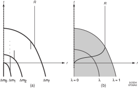
Figure 8: In (a) a discrete sequence of dust shells forms a black hole, and in (b) a continuous version of the same process forms a black hole. These are analogs of Fig. 2 for light.

This elementary result allows us to construct a rather general dust ball with non-uniform density from layers of thin shells. A discrete sequence of thin shells is shown in Fig. 8a. The initial system is a black hole of vanishingly small mass $m_{0}$ with a thin shell of mass $\Delta m_{1}$ collapsing onto it at $t=0$ to give a black hole of mass $m_{1}=m_{0}+\Delta m_{1}$, followed by more shells, and ending with a final shell impacting the origin at $t=\Delta$ to give a final black hole of mass $m_{f}$ and Schwarzschild radius $R=2m_{f}$. In terms of the intermediate masses $m_{j}$ the metric function in the regions between shells is

$$\psi=-\sqrt{2m_{j}/r},\quad\textrm{$j$-th Schwarzschild region}.$$ (77)

The infinite redshift surface where $\psi=-1$ and $g_{00}=0$ is the zigzag line in the figure.

A continuous version of the dust shell sequence is shown in Figure 8b. The shells are labelled by a continuous variable $\lambda$ ranging from 0 to 1, with the total geometric mass inside a shell denoted by $m(\lambda)$; $m(\lambda)$ is the continuum analog of $m_{j}$, and the metric function in the fluid region is thus

$$\psi=-\sqrt{2m(\lambda)/r},\quad\textrm{fluid region}.$$ (78)

The infinite redshift surface is where $\psi=-1$, or

$$r=2m(\lambda),\quad\textrm{infinite redshift surface}.$$ (79)

As in section 3 we label the shells by the total mass inside the shell,

$$m(\lambda)=\lambda m_{f},$$ (80)

where $m_{f}$ is the final mass. The time at which the $\lambda$ shell impacts the center may be chosen rather arbitrarily, and we denote it by $h(\lambda)$. For simplicity and to avoid density singularities it is important that the shells do not cross each other. This will be true if $h(\lambda)$ increases monotonically; that is, outer shells impact at times later than inner shells. Thus we choose $h(\lambda)$ to increase monotonically from 0 to $\Delta$ as $\lambda$ runs from 0 to 1. The equation for the $\lambda$ shell is then the free fall equation for a particle of zero energy, with the particle reaching the origin at $h(\lambda)$, or

$$r^{3/2}+\frac{3}{2}\sqrt{R\lambda}[t-h(\lambda)]=0.$$ (81)

As we will see, the function $h(\lambda)$ determines the dust ball density.

If the function $h(\lambda)$ is specified we can use Eq.(79) and Eq.(80) and Eq.(81) to get a parametric expression for the infinite redshift surface; the radius and time are given in terms of $\lambda$ by

$$r=R\lambda,\quad t=h(\lambda)-\frac{2}{3}R\lambda.$$ (82)

In particular for the central shell with $\lambda=0$, which impacts the center at $t=0$, and the outer shell with $\lambda=1$, which impacts at $t=\Delta$, we have for the infinite redshift surface

$$\begin{array}[]{ll}r=t=0,&\textrm{central shell},\\ r=R,\quad t=\Delta-\frac{2}{3}R,&\textrm{outside shell}.\end{array}$$ (85)

Thus the surface will move outward with time if $\Delta>2R/3$ – that is if the mass impacts the origin sufficiently slowly. Curiously the same expression occurred for the light shell collapse in Eq.(33).

For the special case of zero total impact time, $\Delta=0$, all of the shells impact the center at $t=0$. This is corresponds to the uniform density fluid sphere in the previous section, so $h(\lambda)=0$ clearly implies uniform density. We can explicitly see the relation between $h(\lambda)$ and the density by solving the shell equation Eq.(81) for the mass $m(\lambda)$ inside the shell $\lambda$ at a large negative time $t=-T$, when $T>>h(\lambda)$, to get

$$m(\lambda)=\left[\frac{2}{9(T+h)^{2}}\right]r^{3}\approx\frac{2}{9T^{2}}r^{3}.$$ (86)

Thus in the distant past the mass is proportional to $r^{3}$, meaning that the dust is asymptotically uniform. As time progresses to smaller negative values the density may deviate more and more from uniform, and may be quite non-uniform at $t=0$.

To obtain the metric and other properties of a collapsing dust ball we first specify a function $h$. Then the shell equation Eq.(81) gives the shell parameter as a function of position, that is $\lambda=\lambda(r,t)$. This is consistent because we allow only one shell to pass through a given point. With the parameter known as a function of position the metric in the fluid is given by Eq.(78). With this expression for the shell parameter the shell relation Eq.(81) is an identity in $r,t$.

A number of interesting properties of the dust region may be expressed in terms of the function $h(\lambda)$. (Later we will consider a specific $h(\lambda)$ to illustrate further.) From the expression Eq.(78) for the metric function $\psi$ and $\lambda(r,t)$ we may calculate the Einstein tensor from Eq.(62), obtaining

$$G^{0}_{\;0}=-\frac{R\lambda^{\prime}}{r^{2}},\quad G^{1}_{\;0}=\frac{R\dot{\lambda}}{r^{2}},\quad\lambda^{\prime}=\frac{\partial\lambda}{\partial r},\quad\dot{\lambda}=\frac{\partial\lambda}{\partial t}.\quad$$ (87)

For the other components we need to relate the derivatives $\dot{\lambda}$ and $\lambda^{\prime}$ to each other, which may be done using the shell relation Eq.(81). Differentiating Eq.(81) we find

$$\frac{\partial\sqrt{\lambda}}{\partial r}=\frac{\sqrt{r/R}}{h-t+2\lambda dh/d\lambda},$$

$$\frac{\partial\sqrt{\lambda}}{\partial t}=\frac{\sqrt{\lambda}}{h-t+2\lambda dh/d\lambda},$$

$$\frac{\dot{\lambda}}{\lambda^{\prime}}=\sqrt{\frac{R\lambda}{r}}.$$ (88)

Thus the ratio of derivatives is independent of the function $h$. With the use of Eq.(88) it is only slightly tedious to show that, for any $h$,

$$G^{1}_{\;1}=G^{2}_{\;2}=G^{3}_{\;3}=0.$$ (89)

Thus the pressure terms of the stress-energy tensor are zero, as we expect for dust. Moreover the energy density of the dust is

$$\rho=T^{0}_{\;0}=\frac{R\lambda^{\prime}}{8\pi Gr^{2}},\qquad\textrm{dust region}.$$ (90)

From this we may verify that the total mass of the dust ball is the mass of the final black hole, which we do by again going to large negative times when the dust is in nearly flat space,

$$M_{f}=\int 4\pi r^{2}\rho dr=\frac{R}{2G}\int\lambda^{\prime}dr=\frac{m_{f}}{G}.$$ (91)

Finally the stress energy tensor on the dust ball surface is zero according to Eq.(70) with $n=2/3$.

There are two specific examples of the function $h(\lambda)$ for which Eq.(62) is easily solved. The first example is

$$h(\lambda)=\Delta/\sqrt{\lambda}.$$ (92)

We leave it as an exercise to the reader to show that the metric function in the dust is then

$$\psi=-\frac{\sqrt{r/R}}{2\Delta}\Big{[}t+\sqrt{t^{2}+(8\Delta/3\sqrt{R})r^{3/2}}\Big{]}.$$ (93)

In the limit of $\Delta\to 0$ this gives the same result as Eq.(58 for a uniform dust ball. The energy density is

$$\rho = \frac{\sqrt{R}}{8\pi G\Delta r^{3/2}}\Big{[}\frac{t+\sqrt{t^{2}+(8\Delta/3\sqrt{R})r^{3/2}}}{\sqrt{t^{2}+(8\Delta/3\sqrt{R})r^{3/2}}}\Big{]}$$ (94)

$$\approx 1/(2\pi Gt^{2}),\quad\quad\textrm{for large $t$.}$$

This is a well-behaved positive function with no singularities or zeros for negative $t$.

The second example is

$$h(\lambda)=-D/\sqrt{\lambda},$$ (95)

where $D$ is a constant. This is singular and thus quite different from the first example, and is not represented by Fig.8b: it is singular for $\lambda\to 0$, meaning that the central dust layer collapsed to the center in the infinite past and the outer layer reached the center at time $-D$. We again leave it as an exercise to show that the metric function is

$$\psi=(2r/3t)+\sqrt{R/r}(\Delta/t),$$ (96)

and that the density is

$$\rho=D\sqrt{R}/(4\pi Gt^{2}r^{3/2}).$$ (97)

The singularity at $r=0$ is mild in the sense that the mass inside a sphere goes like $r^{3/2}$. As $t\to 0$ the density approaches infinity as expected. Thus this example represents a dust ball with a mildly singular central density in the distant past, which grows stronger with time until complete collapse, and represents a rather realistic and amusing system Liu .

Finally, we briefly note some properties of light rays in the collapsing dust ball. From the PG metric Eq.(53) we may write the coordinate velocity of light as

$$v_{c}=\frac{dr}{dt}=\left\{\begin{array}[]{cl}1+\psi,&\textrm{outgoing},\\ -1+\psi,&\textrm{infalling}.\end{array}\right.$$ (100)

We generally expect that $\psi$ will be zero at $r=0$, except near $t=0$, so $v_{c}=\pm 1$ there; note that this is not true for the second example considered above. Also, $v_{c}=\pm 1$ for asymptotically large distances. On the infinite redshift surface $\psi=-1$ so that $v_{c}=0$ for outgoing light and $v_{c}=-2$ for infalling light. For the center in the Schwarzschild region $v_{c}=-\infty$. This allows us to make a rough qualitative sketch of some light rays in Fig.9. (For $\Delta=0$ Eq.(100) may be solved exactly.) Note that, as in the case of the thick light shell in Section 3, there is a last light ray out, whose path defines a global horizon inside of which neither particles nor photons may escape to infinity.

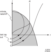
Figure 9: Some “outgoing” light rays in the collapsing dust ball. No ray can escape from the center after the last ray out (B). Compare to Fig. ThickLightShellEFHorizon for light shell collapse.

VII Summary and Further Study

In this paper we have tried to present a simple introduction to the dynamics of gravitational collapse, which we hope can provide a bridge between basic textbook general relativity and numerous research topics of current interest. The light shells in EF coordinates and the fluid spheres in PG coordinates provide the simplest way we know of to study collapse. Some simple but amusing extensions of these models can be made, as already mentioned: one may reverse the time and study the emission of light and matter from white holes or other spherically symmetric objects, and it is easy to add a cosmological constant in the fluid collapse.

The present research literature is dense with studies involving collapse, ranging from fundamental theory to astrophysical applications. A sampling of recent topics from the Los Alamos archives xxx.lanl.gov includes the following, which we paraphrase:

$\bullet$ Entropy in collapse to a black hole - where does the information go?

$\bullet$ Unitarity - is collapse consistent with unitary quantum evolution?

$\bullet$ Cosmic censorship - are all singularities surrounded by a horizon?

$\bullet$ Collapse in context of string theory, anti de Sitter space

$\bullet$ Quantization and entropy of the surface of a black hole.

$\bullet$ Collapse in diverse dimensions.

$\bullet$ Scalar tensor (or other) gravity theories and collapse

$\bullet$ Collapse with a cosmological constant included.

$\bullet$ Particle production in collapse.

$\bullet$ Role of pressure (radial or tangential) in collapse.

$\bullet$ Stability of stars against collapse due to rotation.

$\bullet$ Gravitational radiation from (non-spherical) collapse.

VIII Acknowledgement

This work was supported by NASA grant 8-39225 to Gravity Probe B, and by the US Department of Energy under Contract No. DE-AC02-76SF00515. We thank the members of the Gravity Probe B theory group for many critical and stimulating discussions, in particular Francis Everitt, Robert Wagoner, and Alex Silbergleit.

References

- (1) See for example P. Davies (ed.), The New Physics, Chapter 3 on ”The Renaissance of General Relativity”, C. Will, and Chapter 6 on ”The New Astrophysics”, M. Longair (Cambridge, 1989).
- (2) A brief overview of such concerns is given in G. Fraser (ed.) The New Physics for the 21st Century, Chapter 3 on ”Gravity”, R. J. Adler (Cambridge, 2004) (in press).
- (3) C. W. Misner, K. S. Thorne, and J. A. Wheeler, Gravitation (Freeman, 1973).
- (4) R. J. Adler, M. Bazin, and M. M. Schiffer, Introduction to General Relativity (McGraw Hill, 1975).
- (5) L. D. Landau, E. M. Lifshitz, The Classical Theory of Fields, 4th revised English ed., (Butterworth Heinemann, 1999).
- (6) H. C. Ohanian, R. Ruffini, Spacetime and Gravitation, (Norton, 1994).
- (7) I. R. Kenyon, General Relativity, (Oxford, 1990).
- (8) S. Weinberg, Gravitation and Cosmology, (Wiley, 1972).
- (9) W. Rindler, Essential Relativity, (Van Nostrand and Reinhold, 1969).
- (10) B. F. Schutz, A First Course in General Relativity, (Cambridge, 1985).
- (11) R. Wald, General Relativity, (U. of Chicago press, 1984).
- (12) R. D’Inverno, Introducing Einstein’s Relativity, (Clarendon, Oxford, 1995).
- (13) M. M. Schiffer, R. J. Adler, J. Mark, C. Sheffield, J. Math. Phys. 14, 52 (1973).
- (14) C. Hillman, ”A Brief History of the Concept of Gravitational Collapse”, http://math.ucr.edu/home/ baez/RelWWW/history.html
- (15) J. R. Openheimer and H. Snyder, Phys. Rev. 56, 455 (1939).
- (16) I. D. Novikov, doctoral dissertation, (Shternberg Astronomical Inst. Moscow, 1963).
- (17) B. K. Harrison, K. S. Thorne, M. Wakano, J. A. Wheeler, Gravitational Theory and Gravitational Collapse, (U. of Chicago Press, 1965). This rather early book is mainly devoted to equilibrium configurations and their stability, with dynamical collapse finally discussed in chapter 11.
- (18) A. S. Eddington, Nature 113, 192 (1924).
- (19) D. Finkelstein, Phys. Rev. D 110, 965 (1958).
- (20) P. Painleve, C. R. Hebd. Acad. Sci. (Paris) 173, 677 (1921).
- (21) A. Gullstrand, Arkiv. Mat. Astron. Fys. 16, 1 (1922).
- (22) M. K. Parikh and F. Wilczek, Phys. Rev. Lett. 85 5042 (2000); arXiv: hep-th/9907001.
- (23) M. Parikh, ”A Secret Tunnel Through the Horizon”, Grav. Research Foundation Essay Competition, 1st place.
- (24) M. D. Kruskal, Phys. Rev. 119, 1743 (1960).
- (25) G. Szekeres, Publ. Mat. Debrecen 7, 285 (1960).
- (26) T. P. Singh, ”Gravitational Collapse, Black Holes, and Naked Singularities”, arXiv:gr-qc/9805066v1.
- (27) P. C. Vaidya, Proc. Ind. Acad. Sci. A33, 246 (1951) and Phys. Rev. 33, 10 (1951).
- (28) K. Lake, Phys. Rev. D 62 027301 (2000); arXiv:gr-qc/0002044.
- (29) S. W. Hawking, Comm. Math. Phys. 43 199 (1975).
- (30) G. W. Gibbons, S. W. Hawking, Phys. Rev. D 15, 2752 (1977).
- (31) S. Hawking, R. Penrose, The Nature of Space and Time, (Princeton, 1996).
- (32) R. J. Adler, D. I. Santiago, Mod. Phys. Lett. A 14, 1371 (1999).
- (33) R. J. Adler, P. Chen, D. I. Santiago, Gen. Rel. Grav. 33, 2101 (2001).
- (34) For a short discussion of relevant coordinate systems see M. Weinstein, Workshop on Light-Cone Physics: Particles and Strings, Trento 2001; arXiv:gr-qc/0111027.
- (35) J. S. Liu, Doctoral Thesis, Department of Physics, Stanford University (2004).