Stationary Black Holes

Abstract

We review the theory of uniqueness of stationary black hole solutions of vacuum Einstein equations.
Keywords: black holes, event horizons, Schwarzschild metric, Kerr metric, no-hair theorems

1 Introduction

In this article we consider a specific class of stationary solutions to the Einstein field equations, which read

$$R_{\mu\nu}-\frac{1}{2}g_{\mu\nu}R=\frac{8\pi G}{c^{4}}T_{\mu\nu}.$$ (1.1)

Here $R_{\mu\nu}$ and $R=g^{\mu\nu}R_{\mu\nu}$ are respectively the Ricci tensor and the Ricci scalar of the spacetime metric $g_{\mu\nu}$, $G$ is the Newton constant and $c$ the speed of light. The tensor $T_{\mu\nu}$ is the stress-energy tensor of matter. Spacetimes, or regions thereof, where $T_{\mu\nu}=0$ are called vacuum.

Stationary solutions are of interest for a variety of reasons. As models for compact objects at rest, or in steady rotation, they play a key role in astrophysics. They are easier to study than non-stationary systems because stationary solutions are governed by elliptic rather than hyperbolic equations. Finally, like in any field theory, one expects that large classes of dynamical solutions approach (“settle down to”) a stationary state in the final stages of their evolution.

The simplest stationary solutions describing compact isolated objects are the spherically symmetric ones. In the vacuum region these are all given by the Schwarzschild family. A theorem of Jebsen, usually attributed to Birkhoff, shows that in the vacuum region any spherically symmetric metric, even without assuming stationarity, belongs to the family of Schwarzschild metrics, parameterized by a mass parameter $m$. Thus, regardless of possible motions of the matter, as long as they remain spherically symmetric, the exterior metric is the Schwarzschild one with some constant $m$, which for usual classical-matter models is positive. This has the following consequence for stellar dynamics: Imagine following the collapse of a cloud of pressureless fluid (“dust”). Within Newtonian gravity this dust cloud will, after finite time, contract to a point at which the density and the gravitational potential diverge. However, this result cannot be trusted as a sensible physical prediction because, even if one supposes that Newtonian gravity is still valid at very high densities, a matter model based on non-interacting point particles is certainly not. Consider, next, the same situation in the Einstein theory of gravity: Here a new question arises, related to the form of the Schwarzschild metric outside of the spherically symmetric body:

$$g=-V^{2}dt^{2}+V^{-2}dr^{2}+r^{2}d\Omega^{2}\;,\quad V^{2}=1-\frac{2Gm}{rc^{2}}\;,\quad t\in\mathbb{R}\;,\ r\in(\frac{2Gm}{c^{2}},\infty)\,.$$ (1.2)

Here $d\Omega^{2}$ is the line element of the standard 2-sphere. When $m>0$ the metric (1.2) is manifestly singular as $r=2m$ is approached (from now on we use units in which $G=c=1$), and there arises the need to understand what happens when the radius $r=2m$ is reached, and crossed.

The first key feature of the metric (1.2) is its stationarity, with Killing vector field $X$ given by $X=\partial_{t}$. A Killing field, by definition, is a vector field the local flow of which generates isometries. An asymptotically flat spacetime is called stationary if there exists a Killing vector field $X$ which approaches $\partial_{t}$ in the asymptotically flat region (where $r$ goes to $\infty$, see below for precise definitions) and generates a one parameter groups of isometries. A spacetime is called static if it is stationary and if the stationary Killing vector $X$ is hypersurface-orthogonal, i.e. $X^{\flat}\wedge dX^{\flat}=0$, where $X^{\flat}=X_{\mu}dx^{\mu}=g_{\mu\nu}X^{\nu}dx^{\mu}$. A spacetime is called axisymmetric if there exists a Killing vector field $Y$, which generates a one parameter group of isometries, and which behaves like a rotation in the asymptotically flat region, with all orbits $2\pi$-periodic. In asymptotically flat spacetimes this implies that there exists an axis of symmetry, that is, a set on which the Killing vector vanishes. Killing vector fields which are a non-trivial linear combination of a time translation and of a rotation in the asymptotically flat region are called stationary-rotating, or helical.

There exists a technique, due independently to Kruskal and Szekeres, of attaching together two regions $r>2m$ and two regions $r<2m$ of the Schwarzschild metric, in a way shown in Figure 1, to obtain a manifold with a metric which is smooth at $r=2m$. In the extended spacetime the hypersurface $\{r=2m\}$ is a null hypersurface ${\mycal E}$, the Schwarzschild event horizon. The stationary Killing vector $X=\partial_{t}$ extends to a Killing vector in the extended spacetime, and becomes tangent to and null on ${\mycal E}$. The global properties of the Kruskal–Szekeres extension of the exterior Schwarzschild spacetime make this spacetime a natural model for a non-rotating black hole.

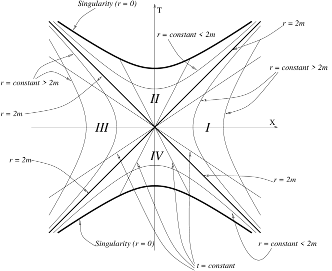
Figure 1: The Kruskal-Szekeres extension of the Schwarzschild solution.

We can now come back to the question of the contracting dust cloud according to the Einstein theory. For simplicity we take the density of the dust to be uniform — the so-called Oppenheimer–Snyder solution. It then turns out that, in the course of collapse, the surface of the dust will eventually cross the Schwarzschild radius, leaving behind a Schwarzschild black hole. If one follows the dust cloud further, a singularity will form, but will not be visible from the ”outside world”, where $r>2m$. For solar-mass objects the Schwarzschild radius is of the order of kilometers, and it is of the order of millions of kilometers for the black hole in the center of our galaxy, so standard phenomenological matter models such as that for dust can still be trusted, and the previous objection to the Newtonian scenario does not apply.

There is a rotating generalization of the Schwarzschild metric, namely the two parameter family of exterior Kerr metrics, which in Boyer-Lindquist coordinates take the form

$$g=-\frac{\Delta-a^{2}\sin^{2}\theta}{\Sigma}dt^{2}-\frac{2a\sin^{2}\theta(r^{2}+a^{2}-\Delta)}{\Sigma}dtd\varphi+{}$$ (1.3)

$${}+\frac{(r^{2}+a^{2})^{2}-\Delta a^{2}\sin^{2}\theta}{\Sigma}\sin^{2}\theta d\varphi^{2}+\frac{\Sigma}{\Delta}dr^{2}+\Sigma d\theta^{2},$$

with $0\leq a<m$. Here $\Sigma=r^{2}+a^{2}\cos^{2}\theta$, $\Delta=r^{2}+a^{2}-2mr$ and $r_{+}<r<\infty$ where $r_{+}=m+(m^{2}-a^{2})^{\frac{1}{2}}$. When $a=0$, the Kerr metric reduces to the Schwarzschild metric (though this is not obvious in the coordinates of (1.3)). The Kerr metric is again a vacuum solution, and it is stationary with $X=\partial_{t}$, the asymptotic time translation, as well as axisymmetric with $Y=\partial_{\varphi}$, the generator of rotations. Similarly to the Schwarzschild case, it turns out that the metric can be smoothly extended across $r=r_{+}$, with $\{r=r_{+}\}$ being a smooth null hypersurface ${\mycal E}$ in a suitable extension. The null generator $K$ of ${\mycal E}$ is the extension of the stationary-rotating Killing field $X+\Omega Y$, where $\Omega=\frac{a}{2mr_{+}}$. On the other hand, the Killing vector $X$ is timelike only outside the hypersurface $\{r=m+(m^{2}-a^{2}\cos^{2}\theta)^{\frac{1}{2}}\}$, on which $X$ becomes null. In the region between $r_{+}$ and $r=m+(m^{2}-a^{2}\cos^{2}\theta)^{\frac{1}{2}}$, which is called the ergoregion, $X$ is spacelike. It is also spacelike on and tangent to ${\mycal E}$, except where the axis of rotation meets ${\mycal E}$, where $X$ is null. By the above properties the Kerr family provides natural models for rotating black holes.

Unfortunately, as opposed to the spherically symmetric case, there are no known explicit collapsing solutions with rotating matter, in particular no known solutions having the Kerr metric as final state.

The aim of the theory outlined below is to understand the general geometrical features of stationary black holes, and to give a classification of models satisfying the field equations.

2 Model independent concepts

We now make precise some notions used informally in the introductory section. The mathematical notion of black hole is meant to capture the idea of a region of spacetime which cannot be seen by “outside observers”. Thus, at the outset, one assumes that there exists a family of physically preferred observers in the spacetime under consideration. When considering isolated physical systems, it is natural to define the “exterior observers” as observers which are “very far” away from the system under consideration. The standard way of making this mathematically precise is by using conformal completions, discussed in more detail in the article about asymptotic structure in this encyclopedia: A pair $(\,\,\,\,\widetilde{\!\!\!\!\mycal M},\,{\tilde{\!g}})$ is called a conformal completion at infinity, or simply conformal completion, of $({\mycal M},g)$ if $\,\,\,\,\widetilde{\!\!\!\!\mycal M}$ is a manifold with boundary such that:

1. ${\mycal M}$ is the interior of $\,\,\,\,\widetilde{\!\!\!\!\mycal M}$,

2. there exists a function $\Omega$, with the property that the metric ${\tilde{g}}$, defined as $\Omega^{2}g$ on ${\mycal M}$, extends by continuity to the boundary of $\,\,\,\,\widetilde{\!\!\!\!\mycal M}$, with the extended metric remaining of Lorentzian signature,

3. $\Omega$ is positive on ${\mycal M}$, differentiable on $\,\,\,\,\widetilde{\!\!\!\!\mycal M}$, vanishes on the boundary

   $${\mycal I}:=\,\,\,\,\widetilde{\!\!\!\!\mycal M}\setminus{\mycal M}\;,$$

   with $d\Omega$ nowhere vanishing on ${\mycal I}$.

The boundary ${\mycal I}$ of $\,\,\,\,\widetilde{\!\!\!\!\mycal M}$ is called Scri, a phonic shortcut for “script I”. The idea here is the following: forcing $\Omega$ to vanish on ${\mycal I}$ ensures that ${\mycal I}$ lies infinitely far away from any physical object — a mathematical way of capturing the notion “very far away”. The condition that $d\Omega$ does not vanish is a convenient technical condition which ensures that ${\mycal I}$ is a smooth three dimensional hypersurface, instead of some, say, one or two dimensional object, or of a set with singularities here and there. Thus, ${\mycal I}$ is an idealized description of a family of observers at infinity.

To distinguish between various points of ${\mycal I}$ one sets

$${\mycal I}^{+}=\{\mbox{points in ${\mycal I}$ which are to the timelike future of the physical spacetime}\}\ .$$

$${\mycal I}^{-}=\{\mbox{points in ${\mycal I}$ which are to the timelike past of the physical spacetime}\}\ .$$

(Recall that a point $q$ is to the timelike future, respectively past, of $p$ if there exists a future directed, respectively past directed, timelike curve from $q$ to $p$. Timelike curves are curves $\gamma$ such that their tangent vector $\dot{\gamma}$ is timelike everywhere, $g(\dot{\gamma},\dot{\gamma})<0$. The set of points related by a future directed timelike curve with a set $\Omega$ is denoted by $I^{+}(\Omega)$. Similarly a curve is causal if $\dot{\gamma}$ is nowhere vanishing, with $g(\dot{\gamma},\dot{\gamma})\leq 0$ everywhere.) One then defines the black hole region ${\mycal B}$ as

$${\mycal B} := \{\mbox{the set of points in ${\mycal M}$ from which}$$ (2.1)

$$\phantom{the}\mbox{no future directed causal curve in $\,\,\,\,\widetilde{\!\!\!\!\mycal M}$ meets ${\mycal I}^{+}$}\}\;.$$

By definition, points in the black hole region cannot send information to ${\mycal I}^{+}$; equivalently, observers on ${\mycal I}^{+}$ cannot see points in ${\mycal B}$. The white hole region ${\mycal W}$ is defined by changing the time orientation in (2.1).

A key notion related to the concept of a black hole is that of future (${\mycal E}^{+})$ and past (${\mycal E}^{-}$) event horizons,

$${\mycal E}^{+}:=\partial{\mycal B}\;,\qquad{\mycal E}^{-}:=\partial{\mycal W}\;.$$ (2.2)

Under assumptions spelled-out below, event horizons in stationary spacetimes with matter satisfying the null energy condition,

$$T_{\mu\nu}\ell^{\mu}\ell^{\nu}\geq 0\quad\mbox{ for all null vectors $\ell^{\mu}$,}$$ (2.3)

are smooth null hypersurfaces, analytic if the metric is analytic.

Indeed, in order to develop a reasonable theory one also needs regularity conditions for the interior of spacetime. These have to be conditions that do not exclude singularities (otherwise the Schwarzschild and Kerr black holes would be excluded), but which nevertheless guarantee a well-behaved exterior region. One such condition, assumed in all the results described below, is the existence in ${\mycal M}$ of an asymptotically flat space-like hypersurface ${\mycal S}$ which is the union of an asymptotic regions diffeomorphic to $\mathbb{R}^{3}$ minus a ball, and of a compact set. One further assumes that either ${\mycal S}$ has no boundary, or the boundary of ${\mycal S}$ lies on $\overline{{\mycal E}^{+}\cup{\mycal E}^{-}}$. To make things precise, for any spacelike hypersurface let $g_{ij}$ be the induced metric, and let $K_{ij}$ denote its extrinsic curvature. A space–like hypersurface ${\mycal S}_{\mathrm{ext}}$ diffeomorphic to ${\mathbb{R}}^{3}$ minus a ball will be called asymptotically flat if the fields $(g_{ij},K_{ij})$ satisfy the fall–off conditions

$$|g_{ij}-\delta_{ij}|+r|\partial_{\ell}g_{ij}|+\cdots+r^{k}|\partial_{\ell_{1}\cdots\ell_{k}}g_{ij}|+r|K_{ij}|+\cdots+r^{k}|\partial_{\ell_{1}\cdots\ell_{k-1}}K_{ij}|\leq Cr^{-1}\ ,$$ (2.4)

for some constants $C$, $k\geq 1$. A hypersurface ${\mycal S}$ (with or without boundary) will be said to be asymptotically flat with compact interior if ${\mycal S}$ is of the form ${\mycal S}_{int}\cup{\mycal S}_{\mathrm{ext}}$, with ${\mycal S}_{int}$ compact and ${\mycal S}_{\mathrm{e}xt}$ asymptotically flat.

There exists a canonical way of constructing a conformal completion with good global properties for stationary spacetimes which are asymptotically flat in the sense of (2.4), and which are vacuum sufficiently far out in the asymptotic region. This conformal completion is referred to as the standard completion and will be assumed from now on.

Given the above completion, the domain of outer communications (d.o.c.) of a black hole spacetime is defined as

$$\langle\langle{\mycal M}\rangle\rangle:={\mycal M}\setminus\{{\mycal B}\cup{\mycal W}\}\;.$$ (2.5)

Thus, $\langle\langle{\mycal M}\rangle\rangle$ is the region lying outside of the white hole region and outside of the black hole region; it is the region which can both be seen by the outside observers and influenced by those. A natural causal regularity condition, which prevents things like existence of closed timelike curves, is to require that $\langle\langle{\mycal M}\rangle\rangle$ be globally hyperbolic, i.e., there exists a spacelike hypersurface which meets every inextendible timelike curve precisely once. This could be, but does not have to, be the hypersurface ${\mycal S}$ above.

Yet another useful condition is that there exists a cross-section of ${\mycal I}^{-}$, say $K$, so that the boundary $\dot{I}^{+}(K)$ of the timelike future of $K$ intersects the future event horizon ${\mycal E}^{+}$ in a compact crosssection.

The collection of all regularity conditions spelled-out so far is known as $I^{+}$-regularity, and it will be assumed in everything that follows.

Returning to the future event horizon, it is now fairly straightforward to show that every Killing vector field $X$ is necessarily tangent to ${\mycal E}^{+}$. As already mentioned, with a considerable amount of work one also proves that ${\mycal E}^{+}$ is a smooth hypersurface. It follows that $X$ is either null or spacelike on ${\mycal E}^{+}$. This leads to a preferred class of event horizons, called Killing horizons. By definition, a Killing horizon associated with a Killing vector $K$ is a null hypersurface which coincides with a connected component of the set

$${\cal H}(K):=\{p\in{\mycal M}:\ g(K,K)(p)=0\;,\ K(p)\neq 0\}\;.$$ (2.6)

A simple example is provided by the “boost Killing vector field” $K=z\partial_{t}+t\partial_{z}$ in Minkowski spacetime: in this case ${\cal H}(K)$ has four connected components

$${\cal H}_{\epsilon\delta}:=\{t=\epsilon z\;,\delta t>0\}\;,\quad\epsilon,\delta\in\{\pm 1\}\;.$$

The closure $\overline{\cal H}$ of ${\cal H}$ is the set $\{|t|=|z|\}$, which is not a manifold, because of the crossing of the null hyperplanes $\{t=\pm z\}$ at $t=z=0$. Horizons of this type are referred to as bifurcate Killing horizons, with the set $\{K(p)=0\}$ called the bifurcation surface of ${\cal H}(K)$. The bifurcate horizon structure in the Kruskal-Szekeres extension of the Schwarzschild spacetime can be clearly seen on Figures 1 and 2.

A careful revisit of a lemma of Vishveshwara and Carter shows that if a Killing vector $K$ is hypersurface-orthogonal, $K^{\flat}\wedge dK^{\flat}=0$, then the set ${\cal H}(K)$ defined in (2.6) is a union of smooth null hypersurfaces, with $K$ being tangent to the null geodesics threading ${\cal H}$ (“${\cal H}$ is generated by $K$”), and so is indeed a Killing horizon. It has been shown by Carter that the same conclusion can be reached if the hypothesis of hypersurface-orthogonality is replaced by that of existence of two linearly independent Killing vector fields.

In stationary-axisymmetric spacetimes a Killing vector $K$ tangent to the generators of a Killing horizon $\cal H$ can be normalised so that $K=X+\Omega Y$, where $X$ is the Killing vector field which asymptotes to a time translation in the asymptotic region, and $Y$ is the Killing vector field which generates rotations in the asymptotic region. The constant $\Omega$ is called the angular velocity of the Killing horizon $\cal H$.

On a Killing horizon ${\cal H}(K)$ one necessarily has

$$\nabla^{\mu}(K^{\nu}K_{\nu})=-2\kappa K^{\mu}.$$ (2.7)

Assuming the so-called dominant energy condition on $T_{\mu\nu}$, it can be shown that $\kappa$ is constant (recall that Killing horizons are always connected in our terminology), it is called the surface gravity of ${\cal H}$. A Killing horizon is called degenerate or extreme when $\kappa=0$, and non–degenerate otherwise; by an abuse of terminology one similarly talks of degenerate black holes, etc. In Kerr spacetimes we have $\kappa=0$ if and only if $m=a$.

The subset of $\langle\langle{\mycal M}\rangle\rangle$ where $X$ is spacelike is called the ergoregion. In the Schwarzschild spacetime we have $\Omega=0$ and the ergoregion is empty, but in Kerr with $a\neq 0$ there is always a nontrivial ergoregion, enclosed by an ergosphere.

A very convenient method for visualising the global structure of spherically symmetric spacetimes is provided by the conformal Carter-Penrose diagrams. An example of such a diagram is provided by Figure 2. Without spherical symmetry such diagrams can sometimes be replaced by projection diagrams, which give a reasonably accurate causal representation of e.g. Kerr metrics.

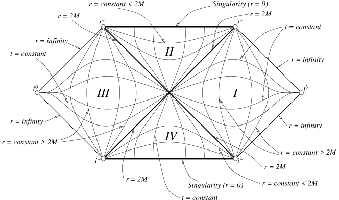
Figure 2: The Carter-Penrose diagram for the Kruskal-Szekeres spacetime. The spacetime contains two asymptotically flat regions, regions $I$ and $III$ in the figure, with corresponding ${\mycal I}^{\pm}$ and ${\mycal E}^{\pm}$ defined with respect to the second region. Each point in this diagram represents a two-dimensional sphere, and coordinates are chosen so that light-cones have slopes plus minus one. Regions are numbered as in Figure 1.

A corollary of the topological censorship theorem of Friedman, Schleich and Witt is that d.o.c.’s of regular black hole spacetimes satisfying the dominant energy condition are simply connected. This implies that connected components of event horizons in stationary spacetimes have ${\mathbb{R}}\times S^{2}$ topology.

We end our review of the concepts associated with stationary black hole spacetimes by summarising the properties of the Schwarzschild and Kerr geometries: The standard textbook extension of the Kerr spacetime with $m>|a|$ is a black hole spacetime with the hypersurface $\{r=r_{+}\}$ forming a non-degenerate, bifurcate Killing horizon generated by the vector field $X+\Omega Y\equiv\partial_{t}+\Omega\partial_{\varphi}$ and surface gravity given by $\kappa=\frac{(m^{2}-a^{2})^{1/2}}{2m[m+(m^{2}-a^{2})^{1/2}]}$. In the case $a=0$, where the angular velocity $\Omega$ vanishes, $X$ is hypersurface-orthogonal and becomes the generator of ${\cal H}$. The bifurcation surface in this case is the totally geodesic 2-sphere, along which the four regions in Figure 1 are joined.

3 Classification of stationary solutions (“No hair theorems”)

We confine attention to the “outside region” of black holes, the domain of outer communications (d.o.c.). For reasons of space we only consider vacuum solutions; there exists a similar theory for electro-vacuum black holes. (There is a somewhat less developed theory for black hole spacetimes in the presence of nonabelian gauge fields, see the review by Gal’tsov and Volkov.) In connection with a collapse scenario the vacuum condition begs the question: collapse of what? The answer is twofold: First, there are large classes of solutions of Einstein equations describing pure gravitational waves. It is believed that sufficiently strong such solutions will form black holes. (Whether or not they will do that is related to the cosmic censorship conjecture, discussed in the article on Spacetime Topology, Global Structure and Singularities in this encyclopedia.) Consider, next, a dynamical situation in which matter is initially present. The conditions imposed in this section correspond then to a final state in which matter has either been radiated away to infinity, or has been swallowed by the black hole (as in the spherically symmetric Oppenheimer–Snyder collapse described above).

Based on the facts below, it is conjectured that the d.o.c.’s of appropriately regular, stationary, vacuum black holes are isometrically diffeomorphic to those of Kerr black holes:

1. The rigidity theorem (key idea by Hawking): event horizons in regular, stationary, analytic vacuum black holes are either Killing horizons, or there exists a second Killing vector in $\langle\langle{\mycal M}\rangle\rangle$.

2. The Killing horizons theorem (Sudarsky-Wald): non–degenerate stationary vacuum black holes such that the event horizon is the union of Killing horizons of the stationary Killing vector are static.

3. Schwarzschild black holes exhaust the family of static regular vacuum black holes (key ideas by Israel and Bunting – Masood-ul-Alam).

4. Kerr black holes satisfying

   $$m^{2}\geq a^{2}$$ (3.1)

   exhaust the family of stationary–axisymmetric, vacuum, connected black holes (key ideas by Carter and Robinson).

The above results are collectively known under the name of no hair theorems, and they have not provided the final answer to the problem so far. Indeed, there are no a priori reasons known for the analyticity hypothesis in the rigidity theorem, except for the non-degenerate slowly-rotating case settled by Alexakis, Ionescu and Klainerman.

Yet another key open question is that of existence of non-connected regular stationary-axisymmetric vacuum black holes. Hennig and Neugebauer have shown that all such configurations with two black-hole components are singular. Regular stationary vacuum configurations with even more components are not expected to exist either. However, there is the following general result of Weinstein: Let $\partial{\mycal S}_{b}$, $b=1,\ldots,N$ be the connected components of $\partial{\mycal S}$. Let $X^{\flat}=g_{\mu\nu}X^{\mu}dx^{\nu}$, where $X^{\mu}$ is the Killing vector field which approaches time translations in the asymptotically flat region. Similarly set $Y^{\flat}=g_{\mu\nu}Y^{\mu}dx^{\nu}$, $Y^{\mu}$ being the Killing vector field associated with rotations. On each $\partial{\mycal S}_{b}$ there exists a constant $\Omega_{b}$ such that the vector $X+\Omega_{b}Y$ is tangent to the generators of the Killing horizon intersecting $\partial{\mycal S}_{b}$. The constant $\Omega_{b}$ is called the angular velocity of the associated Killing horizon. Define

$$\displaystyle m_{b}=-\frac{1}{8\pi}\int_{\partial{\mycal S}_{b}}*dX^{\flat}\ ,$$ (3.2)

$$\displaystyle L_{b}=-\frac{1}{4\pi}\int_{\partial{\mycal S}_{b}}*dY^{\flat}\ .$$ (3.3)

Such integrals are called Komar integrals. One usually thinks of $L_{b}$ as the angular momentum of each connected component of the black hole. Set

$$\mu_{b}=m_{b}-2\Omega_{b}L_{b}\;.$$ (3.4)

Weinstein showed that one necessarily has $\mu_{b}>0$. The problem at hand can be reduced to a harmonic map equation, also known as the Ernst equation, involving a singular map from $\mathbb{R}^{3}$ with Euclidean metric $\delta$ to the two-dimensional hyperbolic space. Let $r_{b}>0$, $b=1,\ldots,N-1$, be the distance in $\mathbb{R}^{3}$ along the axis between neighboring black holes as measured with respect to the (unphysical) metric $\delta$. Weinstein proved that for non-degenerate regular black holes the inequality (3.1) holds, and that the metric on $\langle\langle{\mycal M}\rangle\rangle$ is determined up to isometry by the $3N-1$ parameters

$$(\mu_{1},\ldots,\mu_{N},L_{1},\ldots,L_{N},r_{1},\ldots,r_{N-1})$$ (3.5)

just described, with $r_{b},\mu_{b}>0$. These results by Weinstein contain the no-hair theorem of Carter and Robinson as a special case. Weinstein also shows that for every $N\geq 2$ and for every set of parameters (3.5) with $\mu_{b},r_{b}>0$, there exists a solution of the problem at hand. It is known that for some sets of parameters (3.5) the solutions will have “strut singularities” between some pairs of neighboring black holes, but the existence of the “struts” for all sets of parameters as above is not known, and is the main open problem in our understanding of stationary and axisymmetric vacuum black holes.

See also: Asymptotic Structure and Conformal Infinity. Black Hole Thermodynamics. Initial Value problem for Einstein Equations. Positive energy Theorem and other inequalities in General Relativity. Spacetime Topology, Causal Structure and Singularities.

Suggestions for further reading: [6, 8, 1, 4, 2, 3, 7, 5]

References

- [1] B. Carter, Black hole equilibrium states, Black Holes (C. de Witt and B. de Witt, eds.), Gordon & Breach, New York, London, Paris, 1973, Proceedings of the Les Houches Summer School.
- [2] P.T. Chruściel, Geometry of black holes, Oxford University Press, 2020.
- [3] P.T. Chruściel, J. Lopes Costa, and M. Heusler, Stationary black holes: Uniqueness and beyond, Living Rev. Rel. 15 (2012), 7, arXiv:1205.6112 [gr-qc].
- [4] S.W. Hawking and G.F.R. Ellis, The large scale structure of spacetime, Cambridge University Press, Cambridge, 1973, Cambridge Monographs on Mathematical Physics, No. 1. MR MR0424186 (54 #12154)
- [5] C.A.R. Herdeiro and E. Radu, Asymptotically flat black holes with scalar hair: a review, Int. J. Mod. Phys. D 24 (2015), 1542014.
- [6] B. O’Neill, The geometry of Kerr black holes, A K Peters, Ltd., Wellesley, MA, 1995. MR 1328643 (96c:83052)
- [7] M.S. Volkov and D.V. Gal′tsov, Gravitating non-abelian solitons and black holes with Yang-Mills fields, Phys. Rep. 319 (1999), 83, arXiv:hep-th/9810070. MR 1720519 (2000h:83066)
- [8] R.M. Wald, General relativity, University of Chicago Press, Chicago, 1984.