Hyperbolicity in Spherical Gravitational Collapse in a Horndeski Theory

Abstract

We numerically study spherical gravitational collapse in shift symmetric Einstein dilaton Gauss Bonnet (EdGB) gravity. We find evidence that there are open sets of initial data for which the character of the system of equations changes from hyperbolic to elliptic type in a compact region of the spacetime. In these cases evolution of the system, treated as a hyperbolic initial boundary value problem, leads to the equations of motion becoming ill-posed when the elliptic region forms. No singularities or discontinuities are encountered on the corresponding effective “Cauchy horizon”. Therefore it is conceivable that a well-posed formulation of EdGB gravity (at least within spherical symmetry) may be possible if the equations are appropriately treated as mixed type.

I Introduction

Gravitational wave observation of the binary inspiral of compact objects provides an opportunity to study and test general relativity (GR) in the strong field, dynamical regime. Ideal for such tests are binary black hole (BH) mergers, due to the uniqueness properties of BHs in GR, and that ostensibly their circumbinary environments are sufficiently free of matter to not affect the waveform at a (presently) measurable level. One problem achieving the best possible constraints from current data Abbott et al. (2018) is the dearth of interesting, viable alternatives to GR that can make concrete predictions in the late inspiral and merger regime (see e.g. Yunes et al. (2016)). Specific to this context, by interesting, we mean theories that are consistent with GR in the well-tested weak field regime, yet still predict significant differences for the mergers of BHs; by viable, we mean theories that offer a classically well-posed initial value problem, requisite for computing waveforms to confront with data.

A common scheme to designing modified gravity theories is to add curvature scalars beyond the Ricci scalar $R$ to the Einstein-Hilbert action. The problem with this is typically the resultant classical equations of motion are partial differential equations (PDEs) with higher than second-order derivatives, generically making them Ostrogradsky unstable Woodard (2007, 2015). Two approaches are being pursued to cure this: (1) treating GR as an effective field theory (EFT) and calculating perturbative corrections from the higher order terms Okounkova et al. (2017, 2018); Benkel et al. (2016); Witek et al. (2018); Allwright and Lehner (2018), and (2) modifying the problematic terms in a somewhat ad-hoc fashion inspired by the Israel-Stewart prescription for making relativistic, viscous hydrodynamics well-posed Cayuso et al. (2017). However, there are sub-classes of higher curvature modified gravity theories that still only have second order PDEs, offering the hope that their full, classical equations of motion are well-posed without the need to resort to the above approximation schemes. One such theory is Einstein dilaton Gauss-Bonnet (EdGB) gravity (see e.g. Kanti et al. (1996); Maeda et al. (2009); Yagi et al. (2016) and the references therein), which is the focus of this paper. In particular, we restrict to a version with linear coupling between the scalar field $\phi$ and curvature, which is the simplest member of the shift symmetric class of EdGB theories.

What is interesting about this EdGB gravity theory in the sense of the word discussed above, is that it does not admit the Schwarzschild or Kerr BH solutions of GR. Instead, the analogue BH solutions only exist above a minimum length scale related to the coupling constant $\lambda$ in the theory, and feature scalar “hair” Kanti et al. (1996); Sotiriou and Zhou (2014a, b). Moreover, for values of $\lambda$ that would produce significant changes in stellar mass BHs, the corresponding effect on material compact objects such as neutron stars is insignificant Yagi et al. (2016), implying this theory could be consistent with current GR tests, yet give different results for stellar mass BH mergers. However, it is still unknown under what conditions, if any, EdGB gravity is viable. EdGB gravity can be considered a member of the Horndeski class of scalar-tensor theories Horndeski (1974), though the mapping between the latter form and the one we use here where the Gauss-Bonnet scalar $\mathcal{G}$ is explicit in the action is highly non-trivial Kobayashi et al. (2011). The only systematic study of the well-posedness of EdGB gravity we are aware of Papallo and Reall (2017); Papallo (2017) considered the linearized equations in Horndeski form in the small coupling parameter limit, and found that generically the PDEs are only weakly hyperbolic within a certain class of “generalized harmonic” gauges.

In this work we initiate a study of the hyperbolic properties of 4-dimensional EdGB gravity using numerical solutions of the full equations in the strong field, dynamical regime. As mentioned above, one of our main goals is to ascertain whether EdGB gravity can be relevant for (or constrained with) observable BH mergers. Therefore as a first step toward this goal we restrict to spherically symmetric, asymptotically flat spacetimes, as this is the simplest symmetry reduced setting allowing BH solutions. As in GR, there are no gravitational waves then, and all the dynamics are driven by the scalar field. We thus cannot yet begin to fully address whether BH merger spacetimes are sufficiently “non-generic” to avoid the conclusions reached in the above mentioned studies Papallo and Reall (2017); Papallo (2017) (assuming weak hyperbolicity cannot be lifted to strong hyperbolicity by some novel gauge condition). What we can learn from this study are which scenarios are free of pathologies in spherical symmetry, and use this to guide future studies were we will relax this symmetry restriction.

Our initial survey focused on several regimes, including the weak field/weak coupling limit where an initial concentration of scalar field energy eventually disperses beyond the integration domain, and the strong field/weak coupling regime where the scalar field begins to collapse to a BH (though since our present code uses Schwarzschild-like coordinates we cannot evolve beyond BH formation). In all these cases, which we will discuss in detail in an upcoming paper Ripley and Pretorius (prep), we see no break down in hyperbolicity over the integration domain. Here we present novel results on evolution in the strong field/strong coupling regime, though well below the threshold of black hole formation. In contrast to the weak coupling cases, we find a swath of parameter space where evolution leads to a region of spacetime where the PDEs switch character from hyperbolic to elliptic, implying here the PDEs are actually what is referred to as mixed type. Treated as an initial value problem (IVP), the boundary of the elliptic region is thus effectively a “Cauchy horizon”, beyond which the equations become ill-posed as an IVP (though this is not a Cauchy horizon in the usual sense it is employed in GR, hence the quotes, as the boundary is not null, and from the perspective of the metric the interior and exterior regions are still in causal contact with one another).

Regarding previous work on the dynamical loss of hyperbolicity in solutions of Horndeski theories, this behavior has also been identified at the perturbative level in many Horndeski theories applied to cosmological scenarios (see e.g.Quiros (2019); Kobayashi (2019) and the references therein), though there what we call the elliptic region is usually described as a place where the theory begins to suffer from a “Laplacian” or “gradient” instability. This is a bit of a misnomer as these labels imply some form of physical instability. For with these “instabilities” there either is no problem if an appropriate, physically well-motivated mixed type formulation can be devised, or, as pointed out by Reall et al. (2014); Papallo and Reall (2015) (see also, e.g. Papallo and Reall (2017); Papallo (2017); Ijjas et al. (2019)) the problem is much worse than a physical instability if we demand that the only physically sensible classical theories are those where predictions must be made in the sense of a well-posed IVP. Under the latter condition, initial data within an IVP formulation that leads to an elliptic region would either need to be excluded, or the formation of the elliptic region would need to be regarded as signalling the break down of the theory (as for example singularity formation is in GR).

Researchers investigating the hyperbolicity of higher dimensional Lovelock theories have noted the existence of elliptic regions in black hole and cosmological solutions to those theories. Dimensionally reduced to 4 spacetime dimensions these Lovelock theories can resemble EdGB gravity (see e.g.Charmousis (2015)). The authors in Reall et al. (2014) find that the equations of motion for linear gravitational perturbations of sufficiently small static, spherically symmetric Lovelock black holes are no longer hyperbolic in a region outside the black hole horizon. This may be related to the fact discussed above that EdGB gravity does not have static BH solutions below a certain scale. The authors in Papallo and Reall (2017) show that the dynamical violation of hyperbolicity in Lovelock theories applied to cosmological evolution could in principle occur, although they do not construct explicit solutions where initially hyperbolic equations evolve to form an elliptic region.

An outline of the rest of this paper is as follows. In Sec. II we present the equations of motion of EdGB gravity, along with our choice of coordinates and variables, and the form of the equations we ultimately solve in the code. In Sec. III we outline the calculation of the characteristics of the theory in spherical symmetry. Sec. IV contains results on the class of initial data where evolution can lead to break down of hyperbolicity. We conclude in Sec. V with a discussion of the implications of this for EdGB gravity. We briefly describe our numerical methods and a convergence study in the Appendix, leaving more details and results from different parts of parameter space to Ripley and Pretorius (prep). We work in geometric units and use MTW Misner et al. (1973) sign conventions for the metric tensor, etc.

II Equations of motion

We consider the following EdGB action

$$S=\frac{1}{2}\int d^{4}x\sqrt{-g}\left(R-(\nabla\phi)^{2}+2\lambda\phi\mathcal{G}\right).$$ (1)

The Gauss-Bonnet scalar can be written in terms of the Riemann tensor as $\mathcal{G}\equiv\frac{1}{4}\delta^{\mu\nu\alpha\beta}_{\lambda\sigma\gamma\delta}R^{\lambda\sigma}{}_{\mu\nu}R^{\gamma\delta}{}_{\alpha\beta}$, where $\delta^{\mu\nu\alpha\beta}_{\lambda\sigma\gamma\delta}$ is the generalized Kronecker delta. Varying (1) in turn with respect to the metric $g^{\mu\nu}$ and scalar $\phi$ gives

$$R_{\mu\nu}-\frac{1}{2}g_{\mu\nu}R+2\lambda\delta^{\gamma\delta\kappa\lambda}_{\alpha\beta\rho\sigma}R^{\rho\sigma}{}_{\kappa\lambda}\left(\nabla^{\alpha}\nabla_{\gamma}\phi\right)\delta^{\beta}{}_{(\mu}g_{\nu)\delta}$$

$$-\nabla_{\mu}\phi\nabla_{\nu}\phi+\frac{1}{2}g_{\mu\nu}(\nabla\phi)^{2}=0,$$ (2a)

$$\Box\phi+\lambda\mathcal{G}=0.$$ (2b)

We choose to write the line element in the form

$$ds^{2}=-e^{2A(t,r)}dt^{2}+e^{2B(t,r)}dr^{2}+r^{2}\left(d\vartheta^{2}+\mathrm{sin}^{2}\vartheta d\varphi^{2}\right).$$ (3)

Defining the variables $Q(t,r)\equiv\partial_{r}\phi$ and $P(t,r)\equiv e^{-A+B}\partial_{t}\phi$ , and taking appropriate algebraic combinations of (2b) and the non-trivial components of  (2) results in the following system of PDEs:

$$\Bigg{(}\mathcal{I}^{2}-32\lambda^{2}\mathcal{B}^{2}+128\lambda^{2}e^{-2B}\mathcal{B}\left(1-2\lambda\left(3e^{-2B}+1\right)\frac{Q}{r}\right)\frac{\partial_{r}B}{r}+256\lambda^{3}\mathcal{B}^{2}\left(e^{-2B}\partial_{r}Q-e^{-B}rP\mathcal{K}\right)\Bigg{)}\partial_{r}A$$

$$+ 4\lambda e^{-3B}\mathcal{B}\left(128\lambda^{2}e^{2B}r\mathcal{B}P\mathcal{K}-4\lambda e^{B}P^{2}+e^{B}\left(re^{2B}-12\lambda Q\right)Q\right)\partial_{r}B-512\lambda^{3}re^{-B}\mathcal{B}^{2}\mathcal{K}\partial_{r}P$$

$$- 4\lambda r\mathcal{B}\mathcal{I}\partial_{r}Q-\frac{r\mathcal{B}}{2}\left(e^{2B}+128\lambda^{2}\mathcal{K}^{2}\right)+4\lambda\mathcal{B}\left(-1+128\lambda^{2}\mathcal{K}^{2}\right)Q+2\lambda e^{-2B}Q^{3}$$

$$+ \left(64\lambda^{2}e^{-2B}r\mathcal{B}-16r^{3}\lambda^{2}\mathcal{B}^{2}-\frac{r^{3}}{4}\right)\left(\frac{Q}{r}\right)^{2}+4\lambda r^{2}e^{B}P\mathcal{I}\mathcal{B}\mathcal{K}+\left(16\lambda^{2}r\mathcal{B}^{2}-\frac{r}{4}\mathcal{I}\right)P^{2}=0,$$ (4a)

$$\left(1+4\lambda\left(1-3e^{-2B}\right)\frac{Q}{r}\right)\partial_{r}B-\frac{r}{4}\left(Q^{2}+P^{2}\right)-\frac{1-e^{2B}}{2r}+4\lambda r\mathcal{B}\left(-\partial_{r}Q+re^{B}P\mathcal{K}\right)=0,$$ (4b)

$$\partial_{t}Q-\partial_{r}\left(e^{A-B}P\right)=0,$$ (4c)

$$\left(\mathcal{I}+64\lambda^{2}e^{-2B}\mathcal{B}\frac{\partial_{r}B}{r}\right)\partial_{t}P-\left(\mathcal{I}-64\lambda^{2}e^{-2B}\mathcal{B}\frac{\partial_{r}A}{r}\right)\frac{1}{r^{2}}\partial_{r}\left(r^{2}e^{A-B}Q\right)+16\lambda e^{A-B}\mathcal{I}\left(\frac{\partial_{r}A}{r}\frac{\partial_{r}B}{r}-\mathcal{K}^{2}\right)$$

$$+4\lambda e^{A-B}\mathcal{B}\Bigg{(}\left(P^{2}-Q^{2}\right)+32\lambda rQ\mathcal{K}^{2}-16\lambda e^{-2B}\frac{Q}{r}(\partial_{r}A)^{2}+16\lambda e^{-B}\left(\left(\partial_{r}B-\partial_{r}A\right)P-2\partial_{r}P\right)\mathcal{K}$$

$$+2\frac{\partial_{r}B}{r}+2\left(-1-16\lambda e^{-2B}\frac{Q}{r}-2r\left(1-4\lambda e^{-2B}\frac{Q}{r}\right)\partial_{r}B\right)\frac{\partial_{r}A}{r}\Bigg{)}=0,$$ (4d)

where $\mathcal{B}\equiv(1-e^{-2B})/r^{2}$, $\mathcal{I}\equiv 1-8\lambda e^{-2B}Q/r$, and

$$\mathcal{K} \equiv e^{B}\frac{\frac{PQ}{2}+4\lambda\mathcal{B}\left(-P\partial_{r}B+\partial_{r}P\right)}{e^{2B}+4\lambda\left(-3+e^{2B}\right)\frac{Q}{r}}.$$ (5)

Eqs. (4), though more involved, retain the basic structure of the spherically symmetric Einstein massless-scalar system ($\lambda\to 0$). Namely, (4) and (4b) can be considered constraint equations for the metric variables $A$ and $B$ given data for $P$ and $Q$ on any $t={\rm const.}$ time slice; then (4c) and (4) can be considered evolution equations (where hyperbolic) for $P$ and $Q$. Moreover, as in GR, the system of PDEs (2) is over-determined, and can provide an independent evolution equation for one of the metric functions; we do not solve this equation, rather we monitor its convergence to zero (or more specifically its proxy in the $\vartheta\vartheta$ component of (2)) as a check for the correctness of our solution. Further details on our setup, along with convergence results may be found in the Appendix.

III Characteristics

We follow standard techniques to compute the characteristic structure of our system of PDEs (e.g.Kreiss and Lorenz (1989); Gustafsson et al. (1995); Courant and Hilbert (1962)). For constructing the principal symbol it suffices to only consider the $P,Q$ subsystem, as $A$ and $B$ are fully constrained. We therefore begin by algebraically solving for $\partial_{r}A$, $\partial_{r}B$ in (4,4b) to write (4c,4) as a system of equations of the form

$$E^{(I)}\left[A,B,v^{(J)},\partial_{r}v^{(J)},\partial_{t}v^{(J)}\right] =0,$$ (6)

where $I,J$ run over the labels $(1,2)$, and $v^{(1)}\equiv Q$ and $v^{(2)}\equiv P$. Introducing the characteristic covector $\xi_{a}$, where $a$ runs over the spacetime indices $(t,r)$, the principal symbol is

$$\mathfrak{p}_{J}^{I}(\xi_{a})\equiv\frac{\delta E^{(I)}}{\delta\left(\partial_{a}v^{(J)}\right)}\xi_{a}.$$ (7)

Solving the characteristic equation $\mathrm{det}\left[\mathfrak{p}^{I}_{J}(\xi_{a})\right]=0$ for the characteristic covector, we obtain the following equation for the characteristic speeds $c\equiv-\xi_{t}/\xi_{r}$.

$$c_{\pm}=\frac{1}{2}\left(\mathrm{tr}\left[\mathfrak{c}^{I}_{J}\right]\pm\sqrt{\mathrm{tr}\left[\mathfrak{c}^{I}_{J}\right]^{2}-4\mathrm{det}\left[\mathfrak{c}^{I}_{J}\right]}\right).$$ (8)

where

$$\mathfrak{c}^{I}_{J}\equiv\left(\frac{\delta E^{(I)}}{\delta\left(\partial_{t}v^{(K)}\right)}\right)^{-1}\left(\frac{\delta E^{(K)}}{\delta\left(\partial_{r}v^{(J)}\right)}\right).$$ (9)

The sign of the discriminant $\mathcal{D}$ of Eq. (8) determines the character of the dynamical degree of freedom: when $\mathcal{D}>0$ it is hyperbolic, when $\mathcal{D}=0$ it is parabolic, and when $\mathcal{D}<0$ it is elliptic (when hyperbolic, this $2\times 2$ principal symbol is always strongly hyperbolic in the sense of possessing a complete set of Eigenvectors). In the limit $\lambda=0$, the characteristic speeds reduce to those of GR: $c_{\pm}=\pm e^{A-B}$ and the dynamical degree of freedom is always hyperbolic (for $A$ and $B$ finite and real).

IV Results

We present results from numerical solution of (4) for the following family of initial data

$$\phi(r)|_{t=0}=a_{0}\left(\frac{r}{w_{0}}\right)^{2}\mathrm{exp}\left(-\left(\frac{r-r_{0}}{w_{0}}\right)^{2}\right),$$ (10)

giving $Q|_{t=0}=\partial_{r}\phi|_{t=0}$, and $P$ is chosen to make the initial pulse be approximately ingoing: $P|_{t=0}=-(Q+\phi/r|)_{t=0}$; $a_{0},r_{0}$ and $w_{0}$ are constants.

To characterize the strength of the EdGB modification, we perform the following dimensional analysis. For a compact source of scalar field energy with characteristic length scale $L$, $|\nabla\phi|\sim|\phi_{0}|/L$, where $|\phi_{0}|$ is the maximum difference between $\phi$ and $\phi(t,r=\infty)$ (as we consider a shift symmetric theory). In GR, $|R_{\mu\alpha\nu\beta}|\sim m/L^{3}$, where $m$ is the Arnowitt-Deser-Misner (ADM) mass. Using these expressions to characterize the magnitudes of the various terms in (2), and noting that $\lambda$ has dimension $length^{2}$, we define a dimensionless parameter

$$\eta\equiv \frac{\lambda}{L^{2}}|\phi_{0}|,$$ (11)

so that for $\eta>1$ we expect strong modifications from GR solutions. For the class of initial data above (to within factors of a few) $L\sim w_{0}$ and $|\phi_{0}|\sim a_{0}(r_{0}/w_{0})^{2}$.

The gravitational strength of the initial data can be characterized by the compaction $C\equiv m/L$. Here we present results on cases with large GR-modifications ($\eta\gtrsim 1$), and low ($C\ll 1$) to moderately strong field, but not black hole forming ($C\lesssim 1$). We first show results from one typical case, then a survey confirming the scaling relation (11) above.

IV.1 An example of loss of hyperbolicity when $\eta\gtrsim 1$

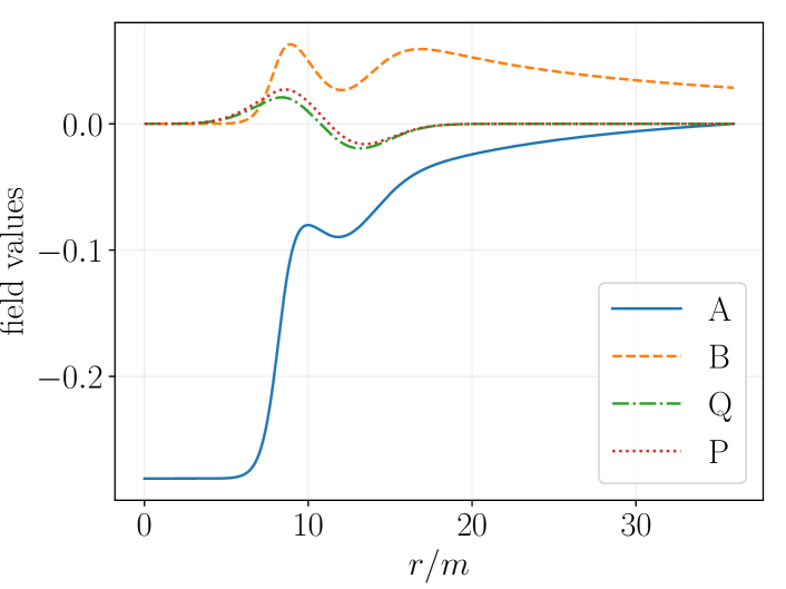
For the specific example, we choose $a_{0}=0.02$, $r_{0}=30$, $w_{0}=10$, and $\lambda=100$. The ADM mass is $m\sim 2.8$. For this initial data, the characteristic speeds are initially real, indicating the scalar field subsystem is hyperbolic. However when $t/m$ reaches $\sim 1.2$, a region forms where the characteristic speeds become imaginary, indicating the character of the equations have become elliptic there—see Fig. 1. Throughout the simulation evolution the spacetime outgoing null characteristic speeds $e^{A-B}$ remain positive and well away from zero, hence the elliptic region is not “censored” by spacetime causal structure. Moreover, at the time the elliptic region first forms, all field variables are smooth and finite—see Fig. 2.

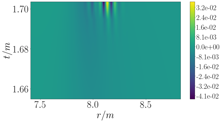
When an elliptic region forms, we expect the PDEs, solved as an IVP, to become ill-posed. The way this is expected to manifest in a numerical hyperbolic solution scheme, as we use, is that short wavelength solution components will begin to grow exponentially, at a rate inversely proportional to their wavelength. Since at the analytic level our initial data is smooth and does not have features smaller than the initial width of the elliptic region, the seeds of the growing modes will come from numerical truncation error. The fastest growing modes are expected to roughly be on order of the mesh spacing of our finite differencing method. Fig. 3 shows such a growing mode just before the code crash at $t/m\sim 1.7$ in this example.

Figure 1: Integral curves of the ingoing (red) and outgoing (blue) characteristic vectors $(1,c_{-})$ and $(1,c_{+})$, respectively.

Figure 2: Field variables at the time ($t/m\sim 1.24$) just before formation of the elliptic region and subsequent loss of convergence.

Figure 3: Plot of $\partial_{r}^{2}P$ inside the elliptic region just before the code crashes. The oscillations occur within the elliptic region—compare the axis scales with that of Fig. 1.

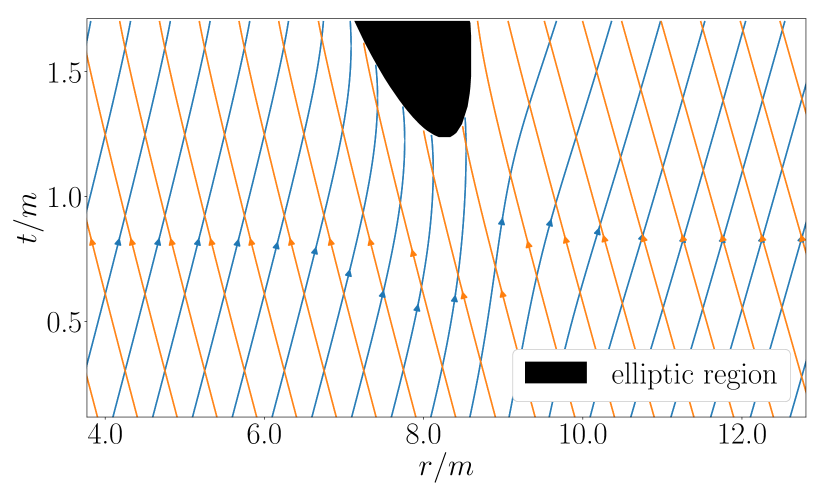
These results imply that the system of PDEs (4) are of mixed type, e.g.Otway (2015); Rassias (1990). Such equations can have regions where the PDEs are hyperbolic, others where they are elliptic, and are parabolic on the co-dimension one surfaces separating these regions, called sonic lines. Given that in Fig.1 it is evident that the characteristics do not intersect the sonic line tangentially, and that the characteristic speeds go to zero on this sonic line, we surmise that at least qualitatively the EdGB equations in this scenario are of Tricomi type (in contrast to Keldysh type where the characteristics meet the sonic line tangentially, and the corresponding speeds diverge there).

Uniqueness results have been obtained for the Tricomi equation Morawetz (1970); Otway (2015), and so one could speculate similar results might hold here. However, given the rather bizarre nature of the boundary conditions needed for the proof (specification of boundary data on a “future” segment within the elliptic region, and free data along only one of the two characteristic surfaces defining the boundary of the hyperbolic region), it is unclear how this could be implemented in a manner that is physically sensible. Moreover, we cannot confidently claim that the picture we have presented here of the sonic line is robust, as strictly speaking in the continuum limit we will only achieve convergence up to the first instant the sonic line is encountered. Even restricting to the purely hyperbolic region uncovered at some fixed resolution, the problem, as mentioned above, is that the elliptic region is not censored. Adding any other matter fields to the problem, or metric perturbations away from spherical symmetry to allow for gravitational waves, will causally connect the elliptic region to the rest of the domain. Therefore, the effective Cauchy horizon here would not be the sonic line, but the boundary of the volume of spacetime in causal contact with the union of elliptic regions.

Another question that arises is to what extent the formation of the elliptic region is gauge invariant. While characteristics are invariant under point transformations (e.g. Courant and Hilbert (1962)), it is less clear that this must be so under full spacetime coordinate transformations, even restricting to manifestly spherical coordinates where $r$ remains an areal radius. The problem then is if we consider a new time coordinate $\bar{t}=\bar{t}(r,t)$, and wish to pose a Cauchy IVP with respect to $\bar{t}$ (and not simply transform the solution from $(t,r)$ to $(\bar{t},r)$), we generically introduce a new gauge degree of freedom (the shift vector $\beta$), and some new PDE must be specified to solve for it. Generically, such a prescription will mix the metric variables with the scalar degree of freedom in a manner where we cannot cleanly separate the gravitational gauge degree of freedom from that of the scalar (or said another way, this will change the rank and structure of the principal symbol in a manner that depends on the PDE describing the gauge). Though it is difficult to imagine how any such coordinate transformation (where $\bar{t}$ continues to define a well-behaved, global time-like foliation) could fundamentally change the PDE character of the scalar degree of freedom, we have yet to devise a proof of this.

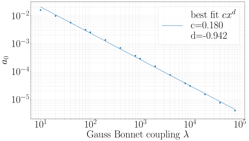
IV.2 Scaling and loss of hyperbolicity

We now show a result from a survey of evolutions, demonstrating that the previous example is not a fine-tuned special case within the initial data family Eq. (10), and that formation of an elliptic region seems to always appear for sufficiently strong coupling, as characterized by $\eta$. For this survey we still keep $w_{0}$ and $r_{0}$ fixed (now $w_{0}=10,r_{0}=20$), but for a given $\lambda$ search for the amplitude parameter $a_{0}$ above which evolution leads to formation of a sonic line (within the run time of the simulations, corresponding to roughly a light-crossing time of the domain). Fig. 4 shows the results, and that the slope of the curve is close to $-1$ suggests the scaling (11) implied by the dimensional analysis does roughly hold in this set up.

Figure 4: Approximate threshold amplitude for the initial data Eq. (10) (with fixed $w_{0}=10,r_{0}=20$) above which evolution leads to the formation of a sonic line, as a function of $\lambda$ (run with a spatial resolution $\Delta r\sim 1\times 10^{-1}$, and the outer boundary at $R_{0}=100$). The ADM mass $m$ scales as $\sim a_{0}^{2}$, and is not particularly sensitive to $\lambda$ in this range of parameter space, hence the vertical axis also serves as an indication of the gravitational strength of the initial data : at $a_{0}\sim 1.6\times 10^{-2}$, $m\sim 0.26$, while at $a_{0}\sim 3\times 10^{-5}$, $m\sim 1\times 10^{-6}$.

V Conclusion

We have presented results from a first study of fully non-linear spherically symmetric gravitational collapse in shift symmetric EdGB gravity. We have shown that for the coupling parameter $\lambda$ sufficiently large, evolution of certain sets of initial data lead to situations where the character of the PDEs governing the dynamical scalar field change from hyperbolic to elliptic in a compact region of the spacetime. This indicates, within these setups, the EdGB equations are of mixed type. For sufficiently weak data, the elliptic region can appear well below the threshold of BH formation, which might otherwise have censored it from asymptotic view. This is problematic for the classical theory to be predictive in the sense of possessing a well-posed Cauchy IVP, at least for arbitrary values of the coupling parameter.

To gain some intuition for what this implies for EdGB gravity serving as a viable modified GR theory to confront with LIGO/Virgo binary BH merger data, we first note that the smallest BH solutions that exist in EdGB gravity have a size $L_{SBH}\sim\sqrt{\lambda}$  Kanti et al. (1996); Sotiriou and Zhou (2014b). Moreover, as modifications to GR BH solutions become less pronounced the larger the BH, we do not want $L_{SBH}\ll O({\rm kms})$ for the theory to remain interesting in this regard. The scaling relation (11) then says we will have hyperbolicity issues for compact distributions of scalar energy on scales $L\lesssim L_{SBH}\sqrt{|\phi_{0}|}$. This is certainly problematic if a putative EdGB scalar has an ambient cosmological background with large density fluctuations. On the other hand, if we assume the cosmological background for $\phi$ is negligible, and (away from scalarized BHs) the only significant levels arise from back-reaction to curvature induced by other matter, a different scaling relation holds. Using similar dimensional analysis to that used to derive (11), one can show that in this case problems arise when the density $\rho$ of “ordinary” matter is greater than $\rho_{SBH}$, the effective density of the smallest BH allowed. If we then choose $\rho_{SBH}$ to be slightly greater than nuclear density (i.e. let the smallest BHs have an effective density slightly larger than that of neutron stars), and ignoring problems that might then need to be addressed in the very early (pre big bang nucleosynthesis) universe, our results do not yet rule out EdGB gravity as being viable and interesting for stellar mass binary BH mergers.

From the EFT perspective, one could argue that for $\eta\sim 1$ we have entered a regime where the truncated theory is no longer valid. That is certainly a sensible stance, but is of little practical use if the higher order terms or full theory are not known. The alternative then is to never approach a regime were the small coupling approximation is violated, but then it is arguable how interesting these theories can remain as models of beyond-GR modifications in binary BH mergers.

In connection to other work (in addition to that already described in the introduction), in Tanahashi and Ohashi (2017) it was argued that for a wide class of Horndeski theories, including EdGB gravity, solutions in spherically symmetric may develop shock-like features in a finite time. Within our class of initial data (10), below the threshold of BH formation, we find no evidence for the unbounded growth of fields or their derivatives before the loss of hyperbolicity of the solution.

We re-emphasize that our characteristic analysis is for the spherically symmetric sector of EdGB gravity, and is tailored to our specific choice of gauge. In particular, in hyperbolic evolution of EdGB gravity in a general four dimensional spacetime there are (expected to be) three, non-gauge, dynamical degrees of freedom. In a spherically symmetric reduction we can say nothing about the dynamics or hyperbolicity of the other two (gravitational) degrees of freedom. There exist covariant notions of the principal symbol (e.g. Christodoulou (2008, 2000); Reall et al. (2014); Papallo and Reall (2017)), from which a covariant notion of hyperbolicity may potentially be derived, be it in a spherically symmetric reduction or a generic four dimensional spacetime. With regards to mixed type behavior, the formation of an elliptic region should reduce the number of dynamical degrees of freedom, which may be apparent from the perspective of the covariant symbol without the need for explicit (numerical) solutions. On the other hand, it is likely that, as we find in the spherically symmetric sector, loss of hyperbolicity depends on the initial data and coupling parameter, and so might not be apparent where it occurs without explicit solutions.

For future work, our next step is to continue the study of spherical collapse in horizon penetrating coordinates, to study under what conditions (if any) the BH solutions remain stable and free of mixed type behavior exterior to the horizons. If viable, we plan to relax the symmetry restrictions to begin addressing the above equations including the gravitational degrees of freedom.

Appendix A Numerical methods and convergence

Here we briefly describe the numerical methods we use, and give one convergence result; more details will be given in an upcoming paper Ripley and Pretorius (prep). We solve (4) using second order finite difference methods. For the results presented here, we implemented the following iterative scheme for each time step. In the evolution equations for $Q$ and $P$ (4c,4), spatial and temporal derivatives are discretized with a Crank-Nicolson stencil. For each time step we: (i) initialize the advanced time level data at $t+\Delta t$ for $A,B,P,Q$ with the known solution at time level $t$; (ii) perform one step of a Newton iteration to solve for a correction to the unknown values of $Q$ and $P$ (4c,4) at the advanced time level, using a banded matrix solver; (iii) integrate the constraints (4,4b) using the trapezoidal rule to solve for $A$ and $B$ at time $t+\Delta t$, and using latest estimates of $P$ and $Q$ from step (ii); (iv) repeat steps (ii) and (iii) until the residual of the full, non-linear set of equations (4) is below a tolerance estimated to be well below truncation error; (v) apply a Kreiss-Oliger dissipation filter Kreiss et al. (1973) to the now known variables at the advanced time. For initial data at $t=0$, we freely specify $P$ and $Q$ as described above, then solve the constraints as in step (iii). As a sanity check that the instabilities we observe at late times are not an artifact of the above time-stepping scheme, we also implemented several other methods, confirming these results, and which we will also describe in Ripley and Pretorius (prep).

Our simulation has a timelike boundary at a fixed radial distance from the origin, $r=R_{0}$. At this outer boundary we imposed outgoing Sommerfeld boundary conditions on the $Q$ and $P$ fields, $\partial_{t}(rQ)+\partial_{r}(rQ)=0$, $\partial_{t}(rP)+\partial_{r}(rP)=0$. As the $A$ and $B$ fields are determined from the first order ordinary differential equations Eqs (4) and (4b), imposing regularity at the origin specifies their behavior over the entire computational domain. Imposing regularity at the origin, where polar coordinates are singular, dictates $\partial_{r}A|_{r=0}=\partial_{r}B|_{r=0}=B|_{r=0}=Q|_{r=0}=\partial_{r}P|_{r=0}=0$. The condition $\partial_{r}B|_{r=0}=0$ is automatically enforced by $B|_{r=0}=Q|_{r=0}=\partial_{r}P|_{r=0}=0$ and (4b). The condition $\partial_{r}A|_{r=0}=0$ is automatically enforced by $B|_{r=0}=\partial_{r}B|_{r=0}=Q|_{r=0}=\partial_{r}P|_{r=0}=0$, and (4). With the coordinates (3) we have the residual gauge freedom to linearly shift $A$ by a function $f(t)$; we use this to set $A(t,R_{0})=0$.

Figure A.1: The $L_{2}$ norm of the $\vartheta\vartheta$ component of Eq. (2). We begin to lose convergence after the formation of the elliptic region (black vertical line; compare with Fig. 1).

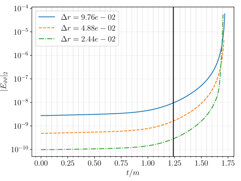
Fig. A.1 shows the $\vartheta\vartheta$ component of the equations of motion for the example described in this paper; we see second order convergence to zero up to and slightly past the formation of the elliptic region. This behavior is typical of the independent residuals for all the different solution techniques we tried. As discussed in the main article, after the formation of the elliptic region, we expect the system of equations solved as a system of hyperbolic PDEs to become ill posed. Short wavelength modes should then grow exponentially, and the fastest growing modes will have wavelengths proportional to the mesh spacing, hence convergence will be lost, and higher resolution simulations will begin to “crash” sooner. What complicates estimating the exact time of blow-up, is since our initial data is smooth, the amplitudes of the short wavelength modes that become unstable in the elliptic region are mostly sourced by truncation error, and so will initially be smaller for higher resolution. In qualitative agreement with these expectations, in Fig. A.1 we observe that the independent residuals of the higher resolution simulations grow more quickly than they do for the lower resolution simulations after the formation of the elliptic region.

References

- Abbott et al. (2018) B. P. Abbott et al. (LIGO Scientific, Virgo), (2018), arXiv:1811.12907 [astro-ph.HE] .
- Yunes et al. (2016) N. Yunes, K. Yagi, and F. Pretorius, Phys. Rev. D94, 084002 (2016), arXiv:1603.08955 [gr-qc] .
- Woodard (2007) R. P. Woodard, The invisible universe: Dark matter and dark energy. Proceedings, 3rd Aegean School, Karfas, Greece, September 26-October 1, 2005, Lect. Notes Phys. 720, 403 (2007), arXiv:astro-ph/0601672 [astro-ph] .
- Woodard (2015) R. P. Woodard, Scholarpedia 10, 32243 (2015), arXiv:1506.02210 [hep-th] .
- Okounkova et al. (2017) M. Okounkova, L. C. Stein, M. A. Scheel, and D. A. Hemberger, Phys. Rev. D96, 044020 (2017), arXiv:1705.07924 [gr-qc] .
- Okounkova et al. (2018) M. Okounkova, M. A. Scheel, and S. A. Teukolsky, (2018), arXiv:1811.10713 [gr-qc] .
- Benkel et al. (2016) R. Benkel, T. P. Sotiriou, and H. Witek, Phys. Rev. D94, 121503 (2016), arXiv:1612.08184 [gr-qc] .
- Witek et al. (2018) H. Witek, L. Gualtieri, P. Pani, and T. P. Sotiriou, (2018), arXiv:1810.05177 [gr-qc] .
- Allwright and Lehner (2018) G. Allwright and L. Lehner, (2018), arXiv:1808.07897 [gr-qc] .
- Cayuso et al. (2017) J. Cayuso, N. Ortiz, and L. Lehner, Phys. Rev. D96, 084043 (2017), arXiv:1706.07421 [gr-qc] .
- Kanti et al. (1996) P. Kanti, N. E. Mavromatos, J. Rizos, K. Tamvakis, and E. Winstanley, Phys. Rev. D54, 5049 (1996), arXiv:hep-th/9511071 [hep-th] .
- Maeda et al. (2009) K.-i. Maeda, N. Ohta, and Y. Sasagawa, Phys. Rev. D80, 104032 (2009), arXiv:0908.4151 [hep-th] .
- Yagi et al. (2016) K. Yagi, L. C. Stein, and N. Yunes, Phys. Rev. D93, 024010 (2016), arXiv:1510.02152 [gr-qc] .
- Sotiriou and Zhou (2014a) T. P. Sotiriou and S.-Y. Zhou, Phys. Rev. Lett. 112, 251102 (2014a), arXiv:1312.3622 [gr-qc] .
- Sotiriou and Zhou (2014b) T. P. Sotiriou and S.-Y. Zhou, Phys. Rev. D90, 124063 (2014b), arXiv:1408.1698 [gr-qc] .
- Horndeski (1974) G. W. Horndeski, International Journal of Theoretical Physics 10, 363 (1974).
- Kobayashi et al. (2011) T. Kobayashi, M. Yamaguchi, and J. Yokoyama, Prog. Theor. Phys. 126, 511 (2011), arXiv:1105.5723 [hep-th] .
- Papallo and Reall (2017) G. Papallo and H. S. Reall, (2017), arXiv:1705.04370 [gr-qc] .
- Papallo (2017) G. Papallo, Phys. Rev. D96, 124036 (2017), arXiv:1710.10155 [gr-qc] .
- Ripley and Pretorius (prep) J. L. Ripley and F. Pretorius, (in prep.).
- Quiros (2019) I. Quiros, (2019), 10.1142/S021827181930012X, arXiv:1901.08690 [gr-qc] .
- Kobayashi (2019) T. Kobayashi, (2019), arXiv:1901.07183 [gr-qc] .
- Reall et al. (2014) H. Reall, N. Tanahashi, and B. Way, Class. Quant. Grav. 31, 205005 (2014), arXiv:1406.3379 [hep-th] .
- Papallo and Reall (2015) G. Papallo and H. S. Reall, JHEP 11, 109 (2015), arXiv:1508.05303 [gr-qc] .
- Ijjas et al. (2019) A. Ijjas, F. Pretorius, and P. J. Steinhardt, JCAP 1901, 015 (2019), arXiv:1809.07010 [gr-qc] .
- Charmousis (2015) C. Charmousis, Proceedings of the 7th Aegean Summer School : Beyond Einstein’s theory of gravity. Modifications of Einstein’s Theory of Gravity at Large Distances.: Paros, Greece, September 23-28, 2013, Lect. Notes Phys. 892, 25 (2015), arXiv:1405.1612 [gr-qc] .
- Misner et al. (1973) C. W. Misner, K. S. Thorne, and J. A. Wheeler, Gravitation (W. H. Freeman, San Francisco, 1973).
- Kreiss and Lorenz (1989) H. Kreiss and J. Lorenz, Initial-boundary Value Problems and the Navier-Stokes Equations, Initial-boundary value problems and the Navier-Stokes equations No. v. 136 (Academic Press, 1989).
- Gustafsson et al. (1995) B. Gustafsson, H. Kreiss, and J. Oliger, Time Dependent Problems and Difference Methods, A Wiley-Interscience Publication (Wiley, 1995).
- Courant and Hilbert (1962) R. Courant and D. Hilbert, Methods of Mathematical Physics, Methods of Mathematical Physics No. v. 2 (Interscience Publishers, 1962).
- Otway (2015) T. Otway, Elliptic–Hyperbolic Partial Differential Equations: A Mini-Course in Geometric and Quasilinear Methods, SpringerBriefs in Mathematics (Springer International Publishing, 2015).
- Rassias (1990) J. Rassias, Lecture Notes on Mixed Type Partial Differential Equations (World Scientific, 1990).
- Morawetz (1970) C. S. Morawetz, Comm. on Pure and Applied Math. 23, 587 (1970).
- Tanahashi and Ohashi (2017) N. Tanahashi and S. Ohashi, Class. Quant. Grav. 34, 215003 (2017), arXiv:1704.02757 [hep-th] .
- Christodoulou (2008) D. Christodoulou, Mathematical Problems of General Relativity I, Mathematical Problems of General Relativity (European Mathematical Society, 2008).
- Christodoulou (2000) D. Christodoulou, “The action principle and partial differential equations. (am-146),” (Princeton University Press, 2000) pp. 220–240.
- Kreiss et al. (1973) H. Kreiss, H. Kreiss, J. Oliger, and G. A. R. P. J. O. Committee, Methods for the approximate solution of time dependent problems, GARP publications series (International Council of Scientific Unions, World Meteorological Organization, 1973).