Process-independent effective coupling and the pion structure function

Abstract

We sketch the calculation of the pion structure functions within the DSE framework, following two alternative albeit consistent approaches, and . discuss then their QCD evolution, the running driven by an effective charge, from a hadronic scale up to any larger one accessible to experiment.

NJU-INP 006/19

1 Introduction

Pions, the Nature’s simplest hadrons, are simultaneously Nambu-Goldstone modes generated by dynamical chiral symmetry breaking in the Standard Model (SM) and bound states of first-generation light quarks and anti-quarks. This key feature explains why symmetries and their breaking play a crucial role in accounting for pions’ properties. More importantly, it is also why charting and understanding pions’ structure and mass distribution in terms of SM strong interactions is a cumbersome, central problem in modern physics, demanding a coherent effort both in QCD continuum and lattice calculations and in experiments shedding a light on this understanding [1].

A basic quantity revealing the pion’s structure is its parton distribution function, ${\mathpzc q}^{\pi}(x;\zeta)$, expressing the probability that a ${\mathpzc q}$-flavour valence quark carries a light-front momentum fraction $x$ in the pion. In particular, this density has been the object of a long controversy, since that leading-order perturbative QCD analysis of $\pi N$ Drell-Yan data (E615 experiment [2]) drew as a conclusion that, at the relevant energy scale for the experiment, $\zeta_{5}$=5.2 GeV, ${\mathpzc q}^{\pi}(x;\zeta_{5})\sim(1-x)$ when $x\to 1$; in clear contradiction with the result early predicted from parton model and perturbative QCD [3, 4, 5]: ${\mathpzc q}^{\pi}(x;\zeta_{H})\sim(1-x)^{2}$, where $\zeta_{H}$ is an energy scale characteristic of nonperturbative dynamics; while QCD evolution is expected to make the exponent increase by the effect of the logarithmic running and thus become effectively $2+\gamma$, with $\gamma\gtrsim 0$, for any scale $\zeta>\zeta_{H}$. Subsequent continuum QCD calculations [6, 7, 8] and further careful re-analyses of E615 data [9, 10], including soft-gluon resummation, have recently reported results consistent with an exponent equal to 2+$\gamma$; while other calculations disregarding symmetry-preserving diagrams [11] or data analysis not yet including relevant threshold resummation effects [12] claimed to have found an exponent closely around 1.

As discussed in Ref. [8], two key issues in determining the pion’s parton distribution function, ${\mathpzc q}^{\pi}(x;\zeta)$, are: (i) accounting, beyond the impulse approximation, for a class of corrections to the handbag-diagram representation of the virtual-photon-pion forward Compton scattering amplitude, restoring basic symmetries in the calculation of parton distributions [7, 13]; and (ii) dealing adequately with the QCD evolution of these parton distributions, from the nonperturbative scale at which they have been obtained up to one accessible to experiment. In the following, we will sketch about (i) and elaborate further on the issue (ii), particularly in connection with a recently proposed process-independent effective charge  [14, 15].

2 The pion parton distribution function

The pion’s parton distribution function can be obtained on the ground of the knowledge of the dressed light-quark propagator and pion Bethe-Salpeter amplitude (BSA), computed by solving the appropriate Dyson-Schwinger and Bethe-Salpeter equations (BSE). In order to keep a natural connection for the renormalisation scale and the reference one for QCD evolution, the Dyson-Schwinger equations (DSE) should be renormalised at a typical hadronic scale, $\zeta_{H}$, where the dressed quasiparticles become the correct degrees-of-freedom [16, 17]. Within this DSE and BSE approach but employing algebraic ansätze, a first study in Ref. [7] yielded some new insight to the calculation by identifying the above-mentioned symmetry-preserving corrections, eventually leading to

$${\mathpzc q}^{\pi}(x;\zeta_{H})=N_{c}{\rm tr}\!\int_{dk}\!\delta_{n}^{x}(k_{\eta})\;n\cdot\partial_{k_{\eta}}\left[\Gamma_{\pi}(k_{\eta},-P)S(k_{\eta})\right]\Gamma_{\pi}(k_{\bar{\eta}},P)\,S(k_{\bar{\eta}})\,,$$ (1)

after implementing the appropriate truncation; where $\int_{dk}:=\int\frac{d^{4}}{(2\pi)^{4}}$ is a Poincaré-invariant regularisation of the integral, $\delta_{n}^{x}(k_{\eta}):=\delta(n\cdot k_{\eta}-xn\cdot P)$; $n$ is a light-like four-vector, $n^{2}=0$, $n\cdot P=-m_{\pi}$; and $k_{\eta}=k+\eta P$, $k_{\bar{\eta}}=k-(1-\eta)P$, $\eta\in[0,1]$; $\Gamma_{\pi}$ is the pion BSA, $S(k)$ is the dressed light-quark propagator, the trace is taken over spinor indices with $N_{c}$=3, such that, if the BSA is canonically normalised, then $\int_{0}^{1}dx{\mathpzc q}^{\pi}(x;\zeta_{H})$=1. Owing to Poincaré covariance, no observable can be expected to depend on $\eta$, i.e. the definition of the relative momentum, and this can be algebraically proved from Eq. (1). Another important property of Eq. (1), that can be made apparent after straightforward algebra, is: ${\mathpzc q}^{\pi}(x;\zeta_{H})={\mathpzc q}^{\pi}(1-x;\zeta_{H})$; which is the consequence of the bound system being described in terms of two identical dressed quasiparticles, in the isospin-symmetric limit.

Then, in a further recent work [17], realistic numerical solutions of both DSE and BSE have been applied to compute the first six Mellin moments of the valence-quark parton distribution, derived from Eq. (1) as follows

$$\langle x^{m}\rangle^{\pi}_{\zeta_{H}}=\int_{0}^{1}dx\,x^{m}{\mathpzc q}^{\pi}(x;\zeta_{H})=\frac{N_{c}}{n\cdot P}{\rm tr}\!\int_{dk}\!\left[\frac{n\cdot k_{\eta}}{n\cdot P}\right]^{m}\Gamma_{\pi}(k_{\bar{\eta}},P)\,S(k_{\bar{\eta}})n\cdot\partial_{k_{\eta}}\left[\Gamma_{\pi}(k_{\eta},-P)S(k_{\eta})\right]\;;\\$$ (2)

the Schlessinger point method (SPM) has been then used to extend this set of moments and thus get a reliable approximant for any moment; and, finally, the SPM-approximant has been applied for the reconstruction of the valence-quark distribution, ${\mathpzc q}^{\pi}(x;\zeta_{H})$ [17]. The parton distribution is therefore fully determined, within this approach, by the kernel interaction specified for both the quark-gap and Bethe-Salpeter equations.

An alternative approach results from the so-called overlap representation, in which the forward limit of the generalised parton distribution gives [18, 19]

$${\mathpzc q}^{\pi}(x;\zeta_{H})=\int\frac{d^{2}{\bf k}_{\perp}}{16\pi^{3}}\;|\psi(x,{\bf k}_{\perp}^{2};\zeta_{H})|^{2}$$ (3)

for the valence-quark parton distribution in terms of the lowest Fock-space light-front wave function (LFWF) at the hadronic scale, $\psi(x,{\bf k}_{\perp}^{2};\zeta_{H})$; its leading-twist contribution resulting from the Bethe-Salpeter wave function, $\chi_{\mu}(k+q,k)=S(k+q)\Gamma_{\pi}(k+q,k)S(k)$, as

$$f_{\pi}\psi(x,{\bf k}^{2}_{\perp})=\mbox{\rm tr}_{\rm CD}\int\frac{d{\bf k}_{\parallel}}{\pi}\;\delta_{n}^{x}(k)\gamma_{5}\gamma\cdot n\;\chi_{\mu}(k-\frac{P}{2},P)\;,$$ (4)

where $f_{\pi}$ is the pion’s leptonic decay constant and the trace is here applied over color and spinor indices. As both the quark propagator and the BSA are in hand, basic ingredients for the realistic computation made in Ref. [17], Eqs. (3,4) can be also implemented to get a realistic estimate for the parton distribution within the DSE approach. Alternatively, one can follow the approach of Ref. [20] and use an appropriate Nakanishi representation of the BSA, such that the LFWF eventually results from a closed expression only involving compact integrals of the so-called Nakanishi weight, a distribution defined on a support $[-1,1]$. Then, this distribution can be adjusted to reproduce the same SPM-approximant Mellin moments of Ref. [17] and, as can be seen in Fig. 2, almost pointwise identical parton distributions at the hadronic scale result from both approaches. One is thus left with a realistic estimate of the LFWF which can be subsequently applied to computing the generalised parton distribution function [21].

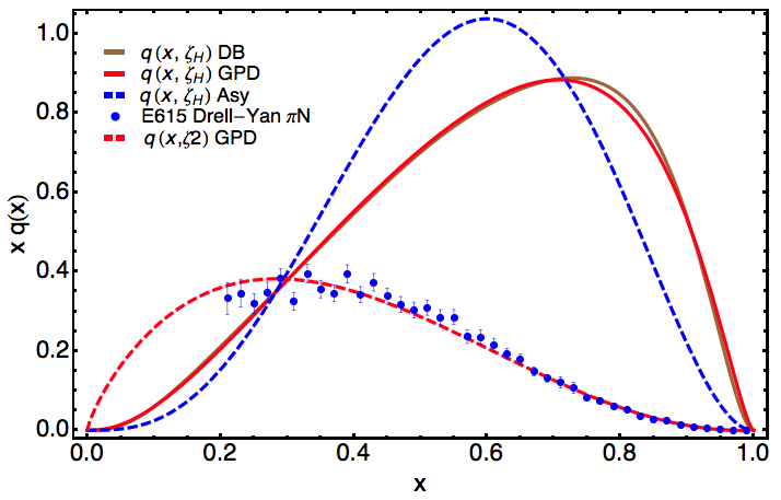
Figure 1: Predicted parton distribution function from Eq. (2) (brown) [8] and from Eq. (3) here (red) and in Ref. [35] (blue dashed) with an algebraic model, both at the hadronic scale $\zeta_{H}$; evolved then up to $\zeta_{5}$ (red dashed), as explained in the text, and successfully compared to reanalysed E615 data [9, 10] (blue circles).

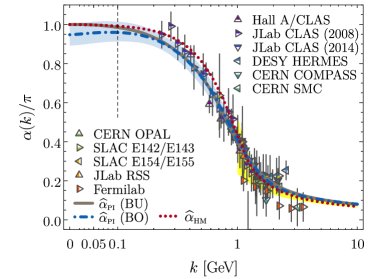
Figure 2: Predicted PI effective charge as obtained in Ref [14] (dot-dashed blue) and improved in Ref. [15], compared to the world’s data of the Bjorken sum-rule charge and to the light-front holographic model (red dotted) canvassed in Ref. [36].

3 DGLAP evolution of hadron structure functions

Once the parton distribution obtained at the hadronic scale, $q^{\pi}(x;\zeta_{H})$, one should employ the QCD-evolution equations to make it evolve up to the relevant scale for E615 and thus obtain $q^{\pi}(x;\zeta_{5})$. The equations describing the scale violations of the hadron structure functions read

$$\left\{\zeta^{2}\frac{d}{d\zeta^{2}}\ -\ \frac{\alpha(\zeta^{2})}{4\pi}\int_{x}^{1}\;\frac{dy}{y}\left(\begin{array}[]{ccc}\displaystyle P_{qq}^{NS}\left(\frac{x}{y}\right)&0&0\\ 0&P_{qq}^{S}\left(\frac{x}{y}\right)&\displaystyle 2n_{f}P_{qG}^{S}\left(\frac{x}{y}\right)\\ 0&\displaystyle P_{Gq}^{S}\left(\frac{x}{y}\right)&\displaystyle P_{GG}^{S}\left(\frac{x}{y}\right)\end{array}\right)\right\}\;\left(\begin{array}[]{c}{\mathpzc q}^{NS}(x;\zeta)\\ q^{S}(y;\zeta)\\ G^{S}(y;\zeta)\end{array}\right)\ =\ 0\ ,$$ (11)

written in terms of integral equations, where ${\mathpzc q}^{NS}$ stands for the non-singlet pure valence-quark and $q^{S}=\sum_{\mathpzc q}{\mathpzc q}+{\overline{\mathpzc q}}$ and $G^{S}$ represent, respectively, the singlet quark and gluon distribution functions in the pion; the elements of the matrix correspond to the so-called splitting functions as can be found, at the leading order, in Ref. [22], and $\alpha(\zeta)$ is the strong running coupling. Then, if the $m$-th order Mellin moment is considered, one is left with

$$\left\{\zeta^{2}\frac{d}{d\zeta^{2}}+\frac{\alpha(\zeta^{2})}{4\pi}\left(\begin{array}[]{ccc}\gamma_{0,qq}^{NS,(m)}&0&0\\ 0&\gamma_{0,qq}^{S,(m)}&2n_{f}\gamma_{qG}^{S,(m)}\\ 0&\gamma_{0,Gq}^{S,(m)}&\gamma_{0,GG}^{S,(m)}\end{array}\right)\right\}\left(\begin{array}[]{c}\langle x_{q}^{m}\rangle_{\zeta}^{NS}\\ \langle x_{q}^{m}\rangle_{\zeta}^{S}\\ \langle x_{G}^{m}\rangle_{\zeta}^{S}\end{array}\right)\ =\ 0\ ;$$ (18)

where the coefficients for the anomalous dimension of the Mellin moments, as defined in (2), result from $\gamma_{0,ij}^{k,(m)}=-\;\int_{0}^{1}\;dx\;x^{m}P_{0,ij}^{k}(x)$ with $i,j$=$q,G$ and $k$=$S,NS$; and can be also found in Ref. [22] (see Eqs. (71-74)). The first row in the matrix of equation (18) leaves us with the standard one-loop DGLAP valence-quark evolution equation. The 2$\times$2 non-diagonal matrix block in (18) describes the evolution of the singlet components and makes also apparent how gluon and quarks become coupled. Indeed, one only needs to deal with the eigenvalue’s problem for the matrix in Eq. (18), and its solutions can be formally written as

$$\left(\begin{array}[]{cc}1&0\\ 0&{\bf P}^{-1}\end{array}\right)\left(\begin{array}[]{c}\langle x_{q}^{m}\rangle_{\zeta}^{NS}\\ \langle x_{q}^{m}\rangle_{\zeta}^{S}\\ \langle x_{G}^{m}\rangle_{\zeta}^{S}\end{array}\right)\ =\ \exp{\left(-\Gamma_{D}^{(m)}\int_{\ln{\zeta_{0}^{2}}}^{\ln{\zeta^{2}}}dt\;\frac{\alpha(e^{t})}{4\pi}\right)}\left(\begin{array}[]{cc}1&0\\ 0&{\bf P}^{-1}\end{array}\right)\left(\begin{array}[]{c}\langle x_{q}^{m}\rangle_{\zeta_{0}}^{NS}\\ \langle x_{q}^{m}\rangle_{\zeta_{0}}^{S}\\ \langle x_{G}^{m}\rangle_{\zeta_{0}}^{S}\end{array}\right)\ ,$$ (29)

where $\Gamma_{D}^{(m)}={\rm Diag}(\gamma_{0,qq}^{NS,(m)},\lambda_{+}^{(m)},\lambda_{-}^{(m)})$ is the matrix of eigenvalues for Eq. (18) and ${\bf P}$ is the matrix which diagonalizes its 2$\times$2 non-diagonal block and, eventually, couples singlet quark and gluon distributions. At the leading order, $\alpha(\zeta)$ is taken from the integration of the 1-loop $\beta$-function and (29) can be thus displayed in terms of simple analytic expressions featuring the logaritmic running of the moments from $\zeta_{0}$ up to $\zeta$, both scales lying in the perturbative domain. However, our aim here (and so was in Ref. [8]) is evolving the valence-quark parton distribution obtained at a naturally nonperturbative hadronic scale, where the pion is only a bound sate of a dressed quark and a dressed antiquark, up to larger energy scales. To this goal, one can go beyond the leading-order approximation by recognising that an effective charge for the strong coupling in Eq. (11) can be defined such that the higher-order corrections become therein optimally neglected and, in order to make predictions, assuming then a phenomenological correspondence of this charge with a well-known effective coupling.

4 The interaction kernel and the process-independent effective strong coupling

The interaction kernel used to get realistic solutions of the DSE gap equation for the quark propagator and for the BSA in Ref. [8], and to compute thus the valence-quark parton distribution, is the one explained in Refs. [23, 24]. This interaction has been found to coincide, in the infrared domain and within the error uncertainties, with a renormalisation-group-invariant (RGI) running-interaction resulting from contemporary studies of QCD’s gauge sector [25],

$$\mathcal{I}(k^{2})\ =\ k^{2}\widehat{d}(k^{2})\ =\ \frac{\alpha_{\rm T}(k^{2})}{[1-L(k^{2};\zeta^{2})F(k^{2};\zeta^{2})]^{2}}\,,$$ (30)

with $\zeta$ still standing for the renormalisation scale; $\widehat{d}(k^{2})$ is a RGI function, owing to a sensible rearrangement of the diagramatic DSE expansion of the involved QCD Green’s functions, within the approach given by the pinch technique and background field method (PTBFM) [26, 27], as discussed in Ref. [28]; $F$ is the dressing function for the ghost propagator; $L$ is a longitudinal piece of the gluon-ghost vacuum polarisation, playing a key role within the context of the PTBFM approach, and that vanishes at $k^{2}=0$ [28]; and $\alpha_{\rm T}$ stands for the strong running coupling derived from the ghost-gluon vertex [29, 30, 28], also called the “Taylor coupling” [31, 32, 33]. Further, on the ground of this running-interaction as a basic ingredient, the process-independent (PI) effective coupling,

$$\widehat{\alpha}_{\rm PI}(k^{2})=\widehat{d}(k^{2})/\mathpzc{D}(k^{2})$$ (31)

has been introduced and discussed in Refs. [14, 15, 34]; where $1/{\mathpzc D}(k^{2})$ is a mass-dimension-two RGI function defined from the gluon two-point Green’s function, as explained therein. As can be seen in Fig. 2, this PI coupling is also found to describe well the world’s data for the process-dependent Bjorken sum-rule effective charge (the roots of this striking coincidence, which opens a window for a direct experimental measure of the PI charge defined on the QCD’s gauge sector, are largely discussed in Ref. [14]).

Following Ref. [34], the coincidence of the PI effective coupling and the DSE interaction kernel, within the infrared domain, supports the assumption that the parametrisation

$$\frac{\alpha(\zeta^{2})}{4\pi}=\left(\beta_{0}\ln{\left(\frac{m_{\alpha}^{2}+\zeta^{2}}{\Lambda^{2}_{\rm QCD}}\right)}\right)^{-1}\ ,$$ (32)

introduced in Ref. [8], is the best candidate for the effective charge from Eq. (11), where $\Lambda_{\rm QCD}$=234 MeV and $m_{\alpha}$=300 MeV are defined to make it coincides with the PI effective coupling, in the infrared, and smoothly connects with the pQCD tail of the kernel interaction in the ultraviolet. Then, as discussed in Ref. [8], $m_{\alpha}\raise 1.29167pt\hbox{$>$\kern-7.5pt\raise-4.73611pt\hbox{$\sim$}}\Lambda_{\rm QCD}$ is a nonperturbative scale screening the soft gluon modes from interaction, which can be naturally identified with the hadronic scale $\zeta_{H}$. Therefore, plugging (32) into (29), the valence-quark parton distribution can be unambigously evolved from $\zeta_{H}=m_{\alpha}$ up to $\zeta_{5}$, and then succesfully compared with the reanalysed E615 data  [9, 10] (see Fig. 2). Furthermore, at the hadronic scale, the pion is a two-valence-body bound-state with no explicit gluon or sea-quark contribution to the singlet distributions, only from valence dressed-quarks. Thus, QCD evolution effectively driven by (32) applied into (29) can be employed to estimate gluon and sea-quark distributions at any larger energy scale, accessible to experiment. The case for the $m=1$ Mellin moment (momentum fraction average) is particularly simple and the singlet distributions from (29) can be recast as ($N_{f}$=4)

$$\langle x_{q}\rangle^{S}_{\zeta}=\frac{3}{7}+\frac{4}{7}\exp{\left(-\frac{56}{36\pi}\int_{\ln{\zeta_{H}^{2}}}^{\ln{\zeta^{2}}}dt\;\alpha(t)\right)}\,,\;\;\;\langle x_{G}\rangle^{S}_{\zeta}=\frac{4}{7}\left[\rule[0.0pt]{0.0pt}{21.33955pt}1-\exp{\left(-\frac{56}{36\pi}\int_{\ln{\zeta_{H}^{2}}}^{\ln{\zeta^{2}}}dt\;\alpha(t)\right)}\right];$$ (33)

which make apparent that, for $\Lambda_{\rm QCD}^{2}/\zeta^{2}\to 0$, sea-quark and gluon momentum fractions tend logarithmically to 3/4 and 4/7, respectively, while the valence-quark tends to 0 [37].

5 Conclusions

We conclude by shortly sumarising. Continuum predictions for the pointwise behaviour of the pion’s distribution functions for valence-quarks, gluons and sea are now consistently available for the first time, obtained within a Dyson-Schwinger-equations’ approach and owing to the implementation of a symmetry-preserving interaction kernel. To this goal, we capitalised on a QCD’s process-independent effective charge, driving the QCD evolution from a nonperturbative scale, unambigously defined by the freeze-out of interacting gluons, below its dynamical mass, up to any larger scale accessible to experiment. This leads to a parameter-free prediction of the pion’s valence-quark distribution function that is in agreement with a modern analysis of the E615 data. The approach herein sketched can be potentially applied to extend the calculations to the spin-dependent structure functions and, beyond the kinematic forward limit, to the generalised parton distributions.

References

References

- [1] Aguilar A C et al. 2019 (Preprint 1907.08218)
- [2] Conway J S et al. 1989 Phys. Rev. D39 92–122
- [3] Ezawa Z F 1974 Nuovo Cim. A23 271–290
- [4] Farrar G R and Jackson D R 1975 Phys. Rev. Lett. 35 1416
- [5] Berger E L and Brodsky S J 1979 Phys. Rev. Lett. 42 940–944
- [6] Hecht M B, Roberts C D and Schmidt S M 2001 Phys. Rev. C63 025213 (Preprint nucl-th/0008049)
- [7] Chang L, Mezrag C, Moutarde H, Roberts C D, Rodr guez-Quintero J and Tandy P C 2014 Phys. Lett. B737 23–29 (Preprint 1406.5450)
- [8] Ding M, Raya K, Binosi D, Chang L, Roberts C D and Schmidt S M 2019 (Preprint 1905.05208)
- [9] Wijesooriya K, Reimer P E and Holt R J 2005 Phys. Rev. C72 065203 (Preprint nucl-ex/0509012)
- [10] Aicher M, Schafer A and Vogelsang W 2010 Phys. Rev. Lett. 105 252003 (Preprint 1009.2481)
- [11] Bednar K D, Clo t I C and Tandy P C 2018 (Preprint 1811.12310)
- [12] Barry P C, Sato N, Melnitchouk W and Ji C R 2018 Phys. Rev. Lett. 121 152001 (Preprint 1804.01965)
- [13] Mezrag C, Chang L, Moutarde H, Roberts C D, Rodr guez-Quintero J, Sabati F and Schmidt S M 2015 Phys. Lett. B741 190–196 (Preprint 1411.6634)
- [14] Binosi D, Mezrag C, Papavassiliou J, Roberts C D and Rodriguez-Quintero J 2017 Phys. Rev. D96 054026 (Preprint 1612.04835)
- [15] Rodr guez-Quintero J, Binosi D, Mezrag C, Papavassiliou J and Roberts C D 2018 Few Body Syst. 59 121 (Preprint 1801.10164)
- [16] Gao F, Chang L, Liu Y X, Roberts C D and Tandy P C 2017 Phys. Rev. D96 034024 (Preprint 1703.04875)
- [17] Ding M, Raya K, Bashir A, Binosi D, Chang L, Chen M and Roberts C D 2019 Phys. Rev. D99 014014 (Preprint 1810.12313)
- [18] Burkardt M, Ji X d and Yuan F 2002 Phys. Lett. B545 345–351 (Preprint hep-ph/0205272)
- [19] Diehl M 2003 Phys. Rept. 388 41–277 (Preprint hep-ph/0307382)
- [20] Xu S S, Chang L, Roberts C D and Zong H S 2018 Phys. Rev. D97 094014 (Preprint 1802.09552)
- [21] Raya K and et al in preparation.
- [22] Altarelli G and Parisi G 1977 Nucl. Phys. B126 298–318
- [23] Qin S x, Chang L, Liu Y x, Roberts C D and Wilson D J 2011 Phys.Rev. C84 042202 (Preprint 1108.0603)
- [24] Qin S x, Chang L, Liu Y x, Roberts C D and Wilson D J 2012 Phys. Rev. C85 035202 (Preprint 1109.3459)
- [25] Binosi D, Chang L, Papavassiliou J and Roberts C D 2015 Phys. Lett. B742 183–188 (Preprint 1412.4782)
- [26] Cornwall J M 1982 Phys.Rev. D26 1453
- [27] Binosi D and Papavassiliou J 2009 Phys.Rept. 479 1–152 245 pages, 92 figures (Preprint 0909.2536)
- [28] Aguilar A C, Binosi D, Papavassiliou J and Rodriguez-Quintero J 2009 Phys. Rev. D80 085018 (Preprint 0906.2633)
- [29] Sternbeck A et al. 2007 PoS LAT2007 256 (Preprint 0710.2965)
- [30] Boucaud P, De Soto F, Leroy J, Le Yaouanc A, Micheli J, Pène O and Rodríguez-Quintero J 2009 Phys.Rev. D79 014508 (Preprint 0811.2059)
- [31] Blossier B, Boucaud P, Brinet M, De Soto F, Du X et al. 2012 Phys.Rev. D85 034503 (Preprint 1110.5829)
- [32] Blossier B, Boucaud P, Brinet M, De Soto F, Du X, Morenas V, Pene O, Petrov K and Rodriguez-Quintero J 2012 Phys. Rev. Lett. 108 262002 (Preprint 1201.5770)
- [33] Blossier B et al. (ETM Collaboration) 2014 Phys.Rev. D89 014507 (Preprint 1310.3763)
- [34] Binosi D and et al in preparation.
- [35] Chouika N, Mezrag C, Moutarde H and Rodr guez-Quintero J 2018 Phys. Lett. B780 287–293 (Preprint 1711.11548)
- [36] Deur A, Brodsky S J and de Teramond G F 2016 Prog. Part. Nucl. Phys. 90 1–74 (Preprint 1604.08082)
- [37] Altarelli G 1982 Phys. Rept. 81 1