The pion parton distribution function in the valence region

Abstract

The parton distribution function of the pion in the valence region is extracted in a next-to-leading order analysis from Fermilab E-615 pionic Drell-Yan data. The effects of the parameterization of the pion’s valence distributions are examined. Modern nucleon parton distributions and nuclear corrections were used and possible effects from higher twist contributions were considered in the analysis. In the next-to-leading order analysis, the high-$x$ dependence of the pion structure function differs from that of the leading order analysis, but not enough to agree with the expectations of pQCD and Dyson-Schwinger calculations.

The pion has a central role in nucleon and nuclear structure. The pion has not only been used to explain the long-range nucleon-nucleon interaction, but also to explain the flavor asymmetry observed in the quark sea in the nucleon. Experimental knowledge of the parton structure of the pion arises primarily from pionic Drell-Yan scattering Conway et al. (1989); Conway (1987); Badier et al. (1983); Betev et al. (1985) from nucleons in heavy nuclei. Recently, the shape of the extracted pion parton distribution function (PDF) at high-$x$, where $x$ is the fraction of the pion momentum carried by the interacting quark, i.e. Bjorken-$x$, has been questioned Hecht et al. (2001).

The anomalously light pion mass is believed to arise from dynamical chiral symmetry breaking. Any model of the pion must account for its dual role as a quark-antiquark system and the Goldstone boson of dynamical chiral symmetry breaking. Theoretical descriptions of pionic parton structure at high-$x$ disagree. The parton model Farrar and Jackson (1975), perturbative quantum chromodynamics (pQCD) Ji et al. (2005); Brodsky et al. (1995) and some non-perturbative calculations such as Dyson-Schwinger Equation (DSE) models Hecht et al. (2001); Maris and Roberts (2003); Bloch et al. (1999, 2000); Hecht et al. (1999) indicate that the high-$x$ behavior should be near $(1-x)^{a}$, with $a\gtrsim 2$. In contrast, relativistic constituent quark models Frederico and Miller (1994); Szczepaniak et al. (1994), Nambu-Jona-Lasinio models with translationaly invariant regularization Shigetani et al. (1993); Davidson and Ruiz Arriola (1995); Weigel et al. (1999); Bentz et al. (1999), Drell-Yan-West relation Drell and Yan (1970); West (1970) and even duality arguments Melnitchouk (2003) favor a linear high-$x$ dependence of $(1-x)$. Instanton-based models appear to lie in between these two Dorokhov and Tomio (2000). Lattice calculations yield only the moments of the distributions and not the PDFs themselves Best et al. (1997); Detmold et al. (2003).

While the PDFs for the nucleon are now well determined by global analyses of a wide range of precise data (see e.g. Lai et al. (2000); Martin et al. (1998); Gluck et al. (1998)) the pion PDFs are very poorly known. Presently there are only two experimental techniques to access quark distributions in the pion: the deep inelastic scattering from the virtual pion cloud of the proton for which data is available in the low-$x$, sea region ($3\times 10^{-4}\leq x\leq 0.01$) Adloff et al. (1999); Chekanov et al. (2002), and the Drell-Yan mechanism which provides data in the valence region ($0.2\leq x\leq 0.99$). Unfortunately there is no overlap between these two experimental techniques.

A previous leading order (LO) analysis of pionic Drell-Yan data by J. Conway et al. (Fermilab E615) Conway et al. (1989) suggested a high-$x$ dependence of $(1-x)^{1.26}$. The data were at relatively high momentum transfer, $Q^{2}>16~{}\rm({GeV})^{2}$, where pQCD should be a valid approach. Previous analyses in both LO Conway et al. (1989); Owens (1984) and next-to-leading order (NLO) Sutton et al. (1992); Gluck et al. (1999) have adopted a simple functional form for the pionic valence quark distributions or made other assumptions about the parton distributions. Since the original analysis of the Drell-Yan data, it has been suggested Hecht et al. (2001) that the simple functional form assigned to the valence quarks in the pion and that using only a LO analysis might introduce a bias at high-$x$.

The purpose of this work is to re-analyze the pionic Drell-Yan cross section data in order to study the high-$x$ behavior of the pion PDFs and to see if such a bias exists. Cross section data from Fermilab E615 (Conway et al.  Conway et al. (1989)) were fit to determine the form of the high-$x$ pion parton distribution. A NLO analysis using the well understood PDFs for the proton (MRST98 Martin et al. (1998), GRV98 Gluck et al. (1998), and CTEQ5M Lai et al. (2000), including nuclear corrections Eskola et al. (1999)) and allowing for higher twist effects was performed.

The LO Drell-Yan cross section for a pion interacting with a nucleon is

$$\frac{d^{2}\sigma}{dx_{\pi}dx_{\rm N}}=\frac{4\pi\alpha^{2}}{9M_{\gamma}^{2}}$$

$$\times\sum e^{2}\left[q_{\pi}(x_{\pi})\bar{q}_{N}(x_{N})+\bar{q}_{\pi}(x_{\pi})q_{N}(x_{N})\right],$$

where the sum is over quark flavor, $q_{\pi{\rm(N)}}$ is the PDF for quark flavor $q$ in the pion (nucleon); $e$ is the charge of the quark, $M_{\gamma}$ is the mass of the virtual photon and $x_{\pi{\rm(N)}}$ is the momentum fraction (Bjorken-$x$) of the interacting quark in the pion (nucleon). (Where not needed for clarity, the subscript “$\pi$” will be dropped.) The cross section per nucleon on an atom with atomic number $Z$ and atomic mass $A$ is

$$\frac{d^{2}\sigma}{dx_{\pi}dx_{\rm N}}=\frac{Z}{A}\frac{d^{2}\sigma^{\rm prot.}}{dx_{\pi}dx_{\rm N}}+\left(1-\frac{Z}{A}\right)\frac{d^{2}\sigma^{\rm neut.}}{dx_{\pi}dx_{\rm N}}.$$ (2)

Charge symmetry (e.g. $u_{\rm prot.}=d_{\rm neut.}$, etc.) was then used to express the cross section in terms of just the pion and proton’s PDFs.

The pion’s valence ($q_{\pi}^{\rm v}$), sea($q_{\pi}^{\rm s}$) and gluonic($g_{\pi}$) parton distributions were parameterized as

$$xq_{\pi}^{\rm v}(x) = A_{\pi}^{\rm v}\left[x^{\alpha}\left(1-x\right)^{\beta}\left(1-\epsilon\sqrt{x}+\nu x\right)\vphantom{\frac{2x^{2}}{9m^{2}_{\mu\mu}}}\right.$$

$$\left.\hphantom{A_{\pi}^{\rm v}\left[\right.}+\gamma\frac{2x^{2}}{9m^{2}_{\gamma\gamma}}\right],$$

$$xq_{\pi}^{\rm s}(x) = A_{\pi}^{\rm s}\left(1-x\right)^{\delta}{\rm~{}and}$$ (4)

$$xg_{\pi}(x) = A^{\rm g}_{\pi}\left(1-x\right)^{\eta},$$ (5)

respectively. The valence parameterization, $xq_{\pi}^{\rm v}$, follows that suggested by Hecht et al. Hecht et al. (2001) with the addition of the term proportional to $x^{2}/m^{2}_{\mu\mu}$ that allows for the possibility of higher-twist effects as suggested by Berger and Brodsky Berger and Brodsky (1979) and used by Conway et al. Conway (1987); Conway et al. (1989). The coefficient of this term, $\gamma$, was restricted to only positive values. This parameterization reduces to the “minimal parameterization” used in earlier works Conway (1987); Conway et al. (1989) if $\epsilon$ and $\nu$ are both fixed at 0. If $\beta=1$, the pion valence PDF has a linear high-$x$ behavior and as $\beta$ increases, there is more curvature at high-$x$. The pion’s sea and gluon distributions are identical to those used in earlier works. We assume the pion’s valence and sea distributions are SU(3) flavor symmetric:

$$xq_{\pi}^{\rm v}(x) = x\bar{u}_{\pi}^{\rm v}(x)=xd_{\pi}^{\rm v}(x){\rm~{}and}$$ (6)

$$xq_{\pi}^{\rm s}(x) = x\bar{u}_{\pi}^{\rm s}(x)=xu_{\pi}^{\rm s}(x)$$

$$= x\bar{d}_{\pi}^{\rm s}(x)=xd_{\pi}^{\rm s}(x)$$

$$= x\bar{s}_{\pi}^{\rm s}(x)=xs_{\pi}^{\rm s}(x).$$

The sea and gluonic distributions are better determined from other data. The shape of the gluon distribution is deduced from CERN WA70 prompt photon data Bonesini et al. (1988). A fit to these data is it best described by $\eta=2.1$ and $G_{\pi}\equiv\int_{0}^{1}xg_{\pi}(x)dx=0.47$ Sutton et al. (1992). The sea distributions can be determined by comparing $\pi^{+}$ and $\pi^{-}$ induced Drell-Yan scattering as was done by the CERN NA3 collaboration who found $\delta=8.4$ Badier et al. (1983). These parameters were fixed at the values given above and were also used by Conway et al. Conway et al. (1989).

Sum rules constrain the normalization coefficients $A^{\rm v}_{\pi}$ and $A^{\rm s}_{\pi}$. Specifically, the total number of valence $\bar{u}$ (and $d$) quarks in the $\pi^{-}$ is constrained to be unity by

$$\int_{0}^{1}q^{\rm v}_{\pi}\left(x_{\pi}\right)dx_{\pi}=1.$$ (8)

Momentum conservation within the pion is enforced by requiring

$$2\int_{0}^{1}xq^{\rm v}_{\pi}\left(x_{\pi}\right)dx_{\pi}+6\int_{0}^{1}\ xq^{\rm s}_{\pi}\left(x_{\pi}\right)dx_{\pi}+G_{\pi}=1.$$ (9)

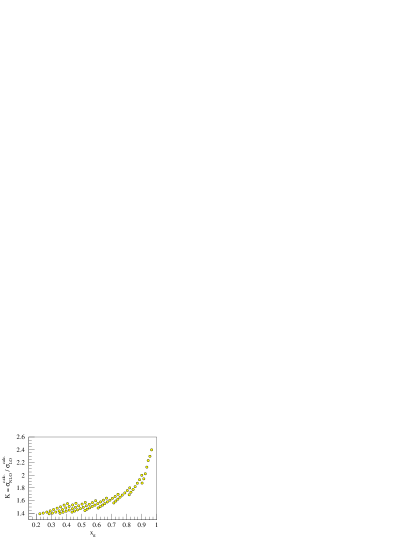
Figure 1: (Color online) The ratio of NLO to LO pionic Drell-Yan cross sections ($K$-factor) calculated using CTEQ5M proton PDF and the pion PDF from this work. One point is shown for each $(x_{F},\sqrt{\tau})$ bin projected onto the $x_{\pi}$ axis. NLO terms are clearly important as $x\rightarrow 1$.

Previous experiments have shown that the basic, LO Drell-Yan cross-section formula fails to explain the magnitude of the observed cross-section, $\sigma^{\rm exp}$, by a factor of nearly two. This is traditionally accounted for by multiplying the LO cross section, $\sigma^{\rm LO}$ by a “$K$”-factor, i.e. $\sigma^{\rm exp}=K\sigma^{\rm LO}$, which is completely independent of kinematics. This difference is attributed to NLO terms and in proton-nucleon Drell-Yan, $K^{\prime}\approx 1$, where $\sigma^{\rm exp}=K^{\prime}\sigma^{\rm NLO}$ Webb et al. (2003). Comparisons of LO and NLO cross section calculations show that the “$K$”-factor is not completely independent of kinematics, in particular in the high-$x$ region, as shown in Fig. 1. Note that $K$ and $K^{\prime}$ are indistinguishable from normalization errors. In the NLO fits, it was assumed that the NLO calculation accounted for the entire observed cross section, and so $K^{\prime}$ reflected the normalization uncertainty. Thus, deviation of $K^{\prime}$ from one contributed to the $\chi^{2}$ of the NLO fits, while $K$ was allowed to vary freely in the LO fits.

The differential cross-section measured by Conway et al. Conway et al. (1989) were the basis for this work. Events arising from $J/\psi$ and $\Upsilon$ decays were removed by requiring that $4.05\leq M_{\gamma}\leq 8.53~{}\textrm{GeV}$. (Relaxing this condition to include bins with $M_{\gamma}\geq 11.06~{}\textrm{GeV}$ had no noticeable effect on the results.) Only bins with $x_{F}\geq 0$ (Feynman-$x$) were included in the fit. Furthermore to minimize the effects of shadowing in copper, only bins in which $x_{\rm N}\geq 0.06$ were used. Finally, if the center of the bin was not within the defined acceptance that bin was not considered by the fit. It is important to note that this final restriction only removed six bins; however, three of these had $x_{\pi}\geq 0.97$. These same restrictions were used in the original fit of these data Conway (1987); Conway et al. (1989). With these restrictions, data from 76 bins of the 168 tabulated in Ref. Conway et al. (1989) remained. The averaged mass for the data included in the fit was 5.2 GeV.

Table 1: Tabulated below are the results from the leading order (LO) and next-to-leading order (NLO) fits at a mass scale of $\langle M_{\gamma}\rangle^{2}=(5.2~{}\textrm{GeV})^{2}$. The original LO fit of Conway et al. Conway et al. (1989) is tabulated in the first column. The second column is a LO fit using the Conway et al. Conway et al. (1989) parameterization of the proton. Succeeding three columns are based on the CTEQ5L parameterization of the proton showing the effects of nuclear corrections and the extended pion PDF parameterization. Following the LO results are the results of the NLO fits. The sixth column gives the results for the full parameterization while the seventh column shows the “minimal” parameterization results (preferred fit). The next two columns give the results for the “minimal” parameterization using the MRST and GRV proton parameterizations. In the final column we see the effect of eliminating the higher twist contributions. In all cases, $\delta$ and $g_{\pi}$ were fixed at $\delta=8.40$ and $g_{\pi}=0.47$.

	Leading Order Fit Results										Next-to-Leading Order Fit Results
Prot. PDF	Fit from		Conway		CTEQ5L		CTEQ5L		CTEQ5L		CTEQ5M		CTEQ5M		MRST98		GRV98		CTEQ5M
Nucl. Corr.	Conway Conway et al. (1989)		-		-		EKS98		EKS98		EKS98		EKS98		EKS98		EKS98		EKS98
$\alpha$	0.60$\pm$	0.03	0.65$\pm$	0.07	0.67$\pm$	0.07	0.67$\pm$	0.07	0.43$\pm$	0.17	0.43$\pm$	0.05	0.70$\pm$	0.06	0.69$\pm$	0.06	0.69$\pm$	0.06	0.66$\pm$	0.04
$\beta$	1.26$\pm$	0.04	1.33$\pm$	0.08	1.35$\pm$	0.08	1.36$\pm$	0.08	1.38$\pm$	0.26	1.60$\pm$	0.08	1.54$\pm$	0.08	1.54$\pm$	0.08	1.53$\pm$	0.08	1.46$\pm$	0.04
$\epsilon$	0.00		0.00		0.00		0.00		-3.39$\pm$	7.02	-3.30$\pm$	1.90	0.00		0.00		0.00		0.00
$\nu$	0.00		0.00		0.00		0.00		-0.76$\pm$	5.52	-0.01$\pm$	1.35	0.00		0.00		0.00		0.00
$\gamma$	0.83$\pm$	0.26	0.78$\pm$	0.65	0.75$\pm$	0.63	0.77$\pm$	0.62	3.0$\pm$	2.8	3.0$\pm$	2.0a	0.60$\pm$	0.34	0.57$\pm$	0.34	0.57$\pm$	0.34	0.00
$K$ ($K^{\prime}$)	1.75$\pm$	0.13	1.57$\pm$	0.11	1.53$\pm$	0.10	1.49$\pm$	0.10	1.56$\pm$	0.24	1.02$\pm$	0.05	0.97$\pm$	0.06	0.98$\pm$	0.06	0.98$\pm$	0.06	1.01$\pm$	0.05
$\chi^{2}/N_{DF}$	359/329		67.6/72		67.1/72		69.3/72		69.1/70		72.8/70		73.1/72		72.0/72		70.9/72		74.4/73

The data were fit in both NLO and LO. In both cases, no QCD evolution was performed so that the resulting pion PDFs are at the average mass scale of the data, $\langle M_{\gamma}\rangle^{2}=(5.2~{}\textrm{GeV})^{2}$. The LO fits were used to compare with the fit of Conway et al. Conway et al. (1989) and so that the effects of the NLO terms in the cross section could be clearly understood. The results shown in Tab. 1. All of the LO fits have slightly more curvature at high-$x$ than the original fit of these data Conway et al. (1989). This includes the one that used the Conway parameterization of the proton. The original work by Conway et al. was based on a finer binning of the data, but the largest differences between the two fits are in the $K$-factor. In this context, it should be noted that a direct calculation based on Conway et al.’s parameterizations of the proton and pion reveal that $K=\sigma_{NLO}/\sigma_{LO}\approx 1.5$ in close agreement with the present fit and a kinematic dependence similar to that in Fig. 1. Fixing $K=1.75$, more closely reproduces Conway et al.’s fit with $\alpha=0.56\pm 0.01$ and $\beta=1.24\pm 0.05$. The use of modern parton distributions and the inclusion of nuclear corrections have only a slight effect on the high-$x$ PDF. In LO when $\epsilon$ and $\nu$ were allowed to freely vary there were significant correlations between fit parameters with $\epsilon$ becoming large and negative while $\gamma$ became large and positive for trivial gains in $\chi^{2}$. A bound of $0<\gamma<3.0$ was implemented in the fit. The shallowness of the $\chi^{2}$ hyper-surface is evident in the large uncertainties in these parameters.

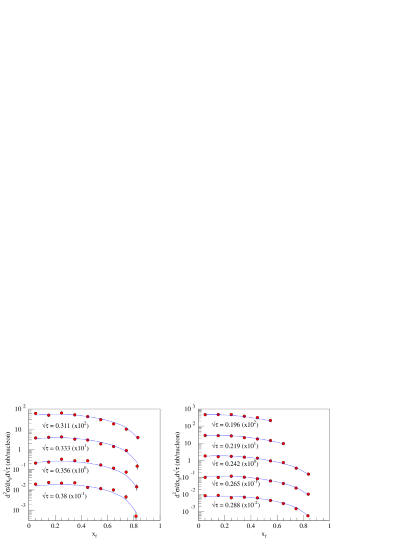
Figure 2: (Color online) Measured values of $d\sigma/dx_{F}d\sqrt{\tau}$ (points) reported by Conway et al. Conway et al. (1989) along with the NLO fit to the data (curves).

These fits were repeated in NLO using the CTEQ5M proton parameterization. As expected from the kinematic dependence of the $K$-factor (see Fig. 1) there is even more curvature at high-$x$ in both the “minimal” and full parameterization with $\beta=1.54$ and $\beta=1.60$ respectively. As in the LO case, the fit to the full parameterization was able to offset increases in $\gamma$ (the higher twist term) with changes in $\epsilon$ and $\nu$ for extremely slight gains in $\chi^{2}$. Based on this, and the relatively large uncertainties in these three parameters, it was reasonable to remove either $\gamma$ from the fit or fix $\epsilon=0$ and $\nu=0$. Fixing $\gamma$ at values between $0.0$ and $0.8$ yields fits which have significantly larger uncertainties in $\epsilon$ and $\nu$. Alternatively, $\gamma$ has a direct physical interpretation, while $\epsilon$ and $\nu$ dilute the interpretation of $\beta$ and are merely present to allow for a better representation of the data. While not considered in this work, the angular distributions observed by Conway et al. and by S. Falciano et al. (CERN NA10) Falciano et al. (1986) are better described with the inclusion of the higher twist term. Using the “minimal” parameterization (fixing $\epsilon=0$ and $\nu=0$) and allowing $\gamma$ to vary fits the data as well as allowing all three parameters to vary. In fact, the distributions of residuals as a function of $x$ are nearly identical to the full fit. Based on these considerations, the “minimal” parameterization was adopted as the preferred parameterization. This fit, compared to data is shown in Fig. 2 and the resulting pion valence parton distribution in Fig. 3. To facilitate the comparison of this fit with lattice results, Tab 2 gives the moments, $\int^{1}_{0}x^{n}q^{\rm v}_{\pi}(x)dx$, of the pion’s valence distributions.

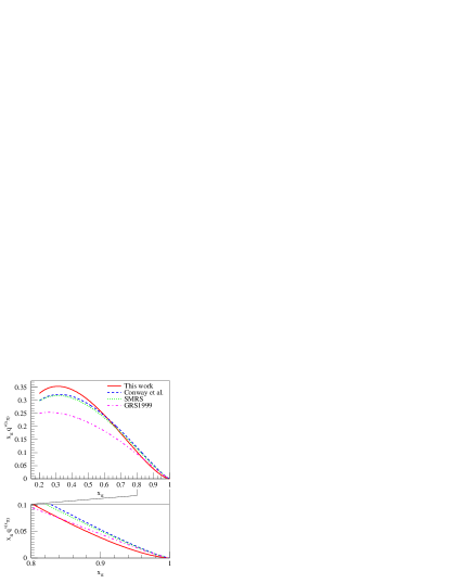
Figure 3: (Color online) The valence pion PDF, $xq^{v}_{\pi}(x)$, for the preferred fit (solid) as well as those from Conway, et al. Conway et al. (1989) (dashed), SMRS Sutton et al. (1992) (dotted) and GRS Gluck et al. (1998) (dot-dashed) at a mass scale of $\langle M_{\gamma}\rangle^{2}=(5.2~{}\textrm{GeV})^{2}$ are shown. The present work shows evidence for greater curvature at high-$x$. The upper plot shows the entire $x$ range of the data, while the lower plot emphasized the high-$x$ region. For comparison, the small higher twist ($\gamma$) term has been removed.

To determine if there was any bias in the fit, it is useful to examine the residual or pull of each data point defined by $R=\left(\sigma^{\rm meas.}-\sigma^{\rm calc.}\right)/\delta^{\rm meas.}$ where $\sigma^{\rm meas.(calc.)}$ is the measured (calculated) cross section and $\delta^{\rm data}$ is the uncertainty of the measured cross section. The distribution of the residuals as a function of $x$ reveals no bias, shown in Fig. 4. The overall distribution is well described by a Gaussian distribution with a standard deviation consistent with unity and mean with zero as shown in Fig. 4.

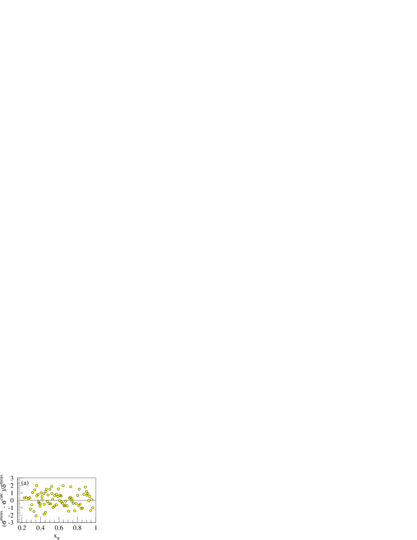
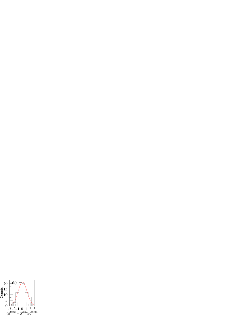
Figure 4: (Color online) (a) The residuals, $R=\left(\sigma^{\rm meas.}-\sigma^{\rm calc.}\right)/\delta^{\rm meas.}$, for the preferred fit as a function of $x$. No bias is apparent as a function of $x$. (b) The residual distribution fit to a Gaussian with $\langle R\rangle=0.14\pm 0.15$ and $\sigma=1.09\pm 0.14$.

Table 2: The moments of the pion valence PDF, evaluated at a mass scale of $\langle M_{\gamma}\rangle^{2}=(5.2~{}\textrm{GeV})^{2}$, are tabulated below. The $0^{\rm th}$ moment was a constraint of the fit–see Eq. 8.

n	$\displaystyle\int^{1}_{0}x^{n}q^{\rm v}_{\pi}(x)dx$
1	0.217$\pm$	0.011
2	0.087$\pm$	0.005
3	0.045$\pm$	0.003

For comparison of the influence of the proton PDF on the fit, additional NLO fits were performed using the MRST Martin et al. (1998) and GRV98 Gluck et al. (1998) parameterizations. These fits produced results similar to those obtained using the CTEQ parameterization, as shown in Tab. 1.

The contribution of the pion’s strange sea was also investigated. The strength of the pion’s strange sea was varied from being equal to the up and down sea [SU(3) flavor symmetric limit–see Eq. The pion parton distribution function in the valence region] to no strange sea. Since most of the data was in the pion’s valence region, it is not surprising that the strange sea of the pion had little effect on the valence parameterization.

Several earlier works have also considered the data fit by the present work, as shown in Fig. 3. The fit by Conway et al. was in LO and showed less curvature at high-$x$, but Conway even speculated that a NLO fit might yield different results Conway (1987). The fit by SMRS Sutton et al. (1992) looked at this data as well as other pionic data. While this fit was in NLO, it was based on what is now an old description of the proton’s PDFs with a linear, ad hoc nuclear correction. In addition, some of the high-$\tau$ data was excluded from the fit. GRS Gluck et al. (1998) studied the pionic PDF in NLO with the less restrictive parameterization, but this work also invoked “constituent quark independence” which directly relates the pion and proton distributions Gluck et al. (1998), introducing a different possible bias.

We have presented a NLO analysis of Drell-Yan data from Fermilab E-615. When analyzed in NLO, the pions valence PDF clearly have more curvature as $x\rightarrow 1$ than previous leading order fits. This is in worse agreement than previous analysis with the linear dependence expected by NJL models Shigetani et al. (1993); Davidson and Ruiz Arriola (1995); Weigel et al. (1999); Bentz et al. (1999), duality argument Melnitchouk (2003) and the Drell-Yan-West relation Drell and Yan (1970); West (1970). It is not as much as is expected from Dyson-Schwinger Equation based models of the pion Hecht et al. (2001); Maris and Roberts (2003); Bloch et al. (1999, 2000); Hecht et al. (1999) or pQCD Ji et al. (2005); Brodsky et al. (1995), however. Finally, while E615’s resolution in $x$ is not given, the mass resolution for the $J/\psi$ is $\sigma_{M}=0.16~{}\textrm{GeV}$ Conway (1987). This could translate into substantial uncertainty in $x$ as $x\rightarrow 1$, so additional data from a more precise experiment with better resolution would certainly be welcome.

We thank C.D. Roberts and W. Melnitchouk for many useful discussions and W. Tung of CTEQ for providing the code necessary for the NLO Drell-Yan cross section calculation. This work was supported by the U.S. Department of Energy, Office of Nuclear Physics, under Contract No. W-31-109-ENG-38.

References

- Conway et al. (1989) J. S. Conway et al., Phys. Rev. D39, 92 (1989).
- Conway (1987) J. S. Conway, Ph.D. thesis, University of Chicago (1987), Fermilab-thesis-1987-16.
- Badier et al. (1983) J. Badier et al. (NA3), Z. Phys. C18, 281 (1983).
- Betev et al. (1985) B. Betev et al. (NA10), Z. Phys. C28, 9 (1985).
- Hecht et al. (2001) M. B. Hecht, C. D. Roberts, and S. M. Schmidt, Phys. Rev. C63, 025213 (2001), eprint nucl-th/0008049.
- Farrar and Jackson (1975) G. R. Farrar and D. R. Jackson, Phys. Rev. Lett. 35, 1416 (1975).
- Ji et al. (2005) X.-d. Ji, J.-P. Ma, and F. Yuan, Phys. Lett. B610, 247 (2005), eprint hep-ph/0411382.
- Brodsky et al. (1995) S. J. Brodsky, M. Burkardt, and I. Schmidt, Nucl. Phys. B441, 197 (1995), eprint hep-ph/9401328.
- Maris and Roberts (2003) P. Maris and C. D. Roberts, Int. J. Mod. Phys. E12, 297 (2003), eprint nucl-th/0301049.
- Bloch et al. (1999) J. C. R. Bloch, C. D. Roberts, S. M. Schmidt, A. Bender, and M. R. Frank, Phys. Rev. C60, 062201 (1999), eprint nucl-th/9907120.
- Bloch et al. (2000) J. C. R. Bloch, C. D. Roberts, and S. M. Schmidt, Phys. Rev. C61, 065207 (2000), eprint nucl-th/9911068.
- Hecht et al. (1999) M. B. Hecht, C. D. Roberts, and S. M. Schmidt, in Proceedings of the workshop on light-cone QCD and Nonperturbative hadron physics (1999), eprint nucl-th/0005067.
- Frederico and Miller (1994) T. Frederico and G. A. Miller, Phys. Rev. D50, 210 (1994).
- Szczepaniak et al. (1994) A. Szczepaniak, C.-R. Ji, and S. R. Cotanch, Phys. Rev. D49, 3466 (1994), eprint hep-ph/9309284.
- Shigetani et al. (1993) T. Shigetani, K. Suzuki, and H. Toki, Phys. Lett. B308, 383 (1993), eprint hep-ph/9402286.
- Davidson and Ruiz Arriola (1995) R. M. Davidson and E. Ruiz Arriola, Phys. Lett. B348, 163 (1995).
- Weigel et al. (1999) H. Weigel, E. Ruiz Arriola, and L. P. Gamberg, Nucl. Phys. B560, 383 (1999), eprint hep-ph/9905329.
- Bentz et al. (1999) W. Bentz, T. Hama, T. Matsuki, and K. Yazaki, Nucl. Phys. A651, 143 (1999), eprint hep-ph/9901377.
- Drell and Yan (1970) S. D. Drell and T.-M. Yan, Phys. Rev. Lett. 24, 181 (1970).
- West (1970) G. B. West, Phys. Rev. Lett. 24, 1206 (1970).
- Melnitchouk (2003) W. Melnitchouk, Eur. Phys. J. A17, 223 (2003), eprint hep-ph/0208258.
- Dorokhov and Tomio (2000) A. E. Dorokhov and L. Tomio, Phys. Rev. D62, 014016 (2000).
- Best et al. (1997) C. Best et al., Phys. Rev. D56, 2743 (1997), eprint hep-lat/9703014.
- Detmold et al. (2003) W. Detmold, W. Melnitchouk, and A. W. Thomas, Phys. Rev. D68, 034025 (2003), eprint hep-lat/0303015.
- Lai et al. (2000) H. L. Lai et al. (CTEQ), Eur. Phys. J. C12, 375 (2000), eprint hep-ph/9903282.
- Martin et al. (1998) A. D. Martin, R. G. Roberts, W. J. Stirling, and R. S. Thorne, Eur. Phys. J. C4, 463 (1998), eprint hep-ph/9803445.
- Gluck et al. (1998) M. Gluck, E. Reya, and A. Vogt, Eur. Phys. J. C5, 461 (1998), eprint hep-ph/9806404.
- Adloff et al. (1999) C. Adloff et al. (H1), Eur. Phys. J. C6, 587 (1999), eprint hep-ex/9811013.
- Chekanov et al. (2002) S. Chekanov et al. (ZEUS), Nucl. Phys. B637, 3 (2002), eprint hep-ex/0205076.
- Owens (1984) J. F. Owens, Phys. Rev. D30, 943 (1984).
- Sutton et al. (1992) P. J. Sutton, A. D. Martin, R. G. Roberts, and W. J. Stirling, Phys. Rev. D45, 2349 (1992).
- Gluck et al. (1999) M. Gluck, E. Reya, and I. Schienbein, Eur. Phys. J. C10, 313 (1999), eprint hep-ph/9903288.
- Eskola et al. (1999) K. J. Eskola, V. J. Kolhinen, and C. A. Salgado, Eur. Phys. J. C9, 61 (1999), eprint hep-ph/9807297.
- Berger and Brodsky (1979) E. L. Berger and S. J. Brodsky, Phys. Rev. Lett. 42, 940 (1979).
- Bonesini et al. (1988) M. Bonesini et al. (WA70), Z. Phys. C37, 535 (1988).
- Webb et al. (2003) J. C. Webb et al. (NuSea) (2003), eprint hep-ex/0302019.
- Falciano et al. (1986) S. Falciano et al. (NA10), Z. Phys. C31, 513 (1986).