Valence-quark distributions in the pion

I Introduction

The cross section for deep inelastic lepton-hadron scattering can be interpreted in terms of the momentum-fraction probability distributions of quarks and gluons (partons) in the hadronic target, and since the pion is a two-body bound state with only $u$- and $d$-valence-quarks it is, in some respects, the simplest hadron and therefore represents the least complicated, nontrivial system for which these distribution functions can be calculated. In a theorist’s ideal world, stable pion targets would then facilitate a comparison between these calculations and the parton distribution functions measured in deep inelastic scattering. However, pion targets are not abundant, and therefore these functions have primarily been inferred from Drell-Yan[1, 2] and direct photon production[3] in pion-nucleon and pion-nucleus collisions: an approach that can only be successful if the nucleon’s parton distributions are well known[4]. More recently, semi-inclusive e p $\to$ e$\,NX$ reactions, $N=p,n$, have also been employed[5], a method which assumes that small-virtuality pions dominate leading nucleon production. These experiments are challenging but high-statistics data exist.

The theoretical situation is arguably poorer: the systematic tool provided by perturbative QCD does not admit the calculation of the distribution functions but only of their evolution from one large spacelike-$q^{2}$ to another; and numerical simulations of lattice-QCD are currently restricted to the quenched approximation and only yield moments of the distributions, not the distributions themselves[6]. Furthermore, the fact that the pion is both a bound state and the Goldstone mode associated with dynamical chiral symmetry breaking complicates the calculation of the pion’s distribution functions and places additional constraints on any framework applied to the task. Considerations of chiral symmetry have led some[7, 8, 9] to adopt the Nambu–Jona-Lasinio model as a basis for their calculations but a number of the difficulties with this approach, among them a marked sensitivity to the regularisation procedure in this non-renormalisable model, are emphasised and discussed in Refs.[8, 9]. Constituent quark models have also been employed[10], with difficulties encountered in such studies considered in Ref.[11]; and so has an instanton-liquid model[12].

The Dyson-Schwinger equations (DSEs)[13] provide an approach well-suited to the calculation of pion observables. Since a chiral symmetry preserving truncation scheme exists[14], they easily capture the dichotomous bound-state/Goldstone-mode character of the pion[15, 16]. Furthermore, because perturbation theory is recovered in the weak coupling limit, they combine; e.g., a description of low-energy $\pi$-$\pi$ scattering[17] with a calculation of the electromagnetic pion form factor, $F_{\pi}(q^{2})$, that yields[18]: the $1/q^{2}$-behaviour expected from perturbative analyses at large spacelike-$q^{2}$ and a calculated evolution to the $\rho$-meson pole in the timelike region[19]. These and other features of contemporary applications are described in Refs.[20, 21].

Herein we employ a phenomenological DSE model, used previously[22, 23] in a description of a wide range of electron-nucleon and meson-nucleon form factors, in a calculation of the pion’s valence-quark distribution. The framework is Poincaré covariant and exhibits, in a simplified form, the features of renormalisability and asymptotic freedom characteristic of QCD. Another important aspect of our study is a description of the pion as a bound state of a dressed-quark and -antiquark through its momentum-dependent Bethe-Salpeter amplitude, with the dressed-quark propagator exhibiting that momentum-dependence characteristic of DSE studies and recently confirmed in simulations[24] of lattice-QCD.

Our article is organised thus: Sec. II recapitulates the calculation of the hadronic tensor for lepton-pion scattering; Sec. III describes the DSE elements necessary in the calculation of the distribution functions – dressed-propagators, Bethe-Salpeter amplitudes, etc.; Sec. IV reports and discusses the results; and Sec. V is an epilogue.

FIG. 1.: “Handbag” contributions to the virtual photon-pion forward Compton scattering amplitude, which are the only impulse approximation diagrams that survive in the deep inelastic Bjorken limit, Eq. (1). $\pi$, dashed-line; $\gamma$, wavy-line; ${\cal S}$, internal solid-line, dressed-quark propagator, Eq. (39). The filled circles represent the pion’s Bethe-Salpeter amplitude, $\Gamma_{\pi}$ in Eq. (LABEL:genpibsa), and the dressed-quark-photon vertex, $\Gamma_{\mu}$ in Eq. (LABEL:bcvtx), depending on which external line they begin/end.

II Lepton-Pion Scattering

Deep inelastic scattering from a pion target can be studied via the diagrams in Fig. 1, which describe virtual photon-pion forward Compton scattering and are[25] the only impulse approximation contributions to survive in the Bjorken limit:

$$q^{2}\to\infty\,,\;\;P\cdot q\to-\infty\;\;\mbox{but}\;\;x:=-\frac{q^{2}}{2P\cdot q}\;\;\mbox{fixed.}$$ (1)

The upper diagram represents the renormalised matrix element

$$T^{+}_{\mu\nu}(q,P)=$$ (4)

$${\rm tr}\!\int\!\frac{d^{4}k}{(2\pi)^{4}}\,\tau_{-}\bar{\Gamma}_{\pi}(k_{\Gamma};-P)\,S(k_{t})\,ieQ\Gamma_{\nu}(k_{t},k)$$

$$\times\,S(k)\,ieQ\Gamma_{\mu}(k,k_{t})\,S(k_{t})\,\tau_{+}\Gamma_{\pi}(k_{\Gamma};P)\,S(k_{s})\,,$$

where: $\Gamma_{\pi}(\ell;P)$ is the pion’s Bethe-Salpeter amplitude and

$$\bar{\Gamma}_{\pi}(\ell;-P)=C^{\dagger}\Gamma_{\pi}(-\ell;-P)^{\rm T}C\,,$$ (5)

with $\tau_{\pm}=\frac{1}{2}(\tau_{1}\pm i\tau_{2})$, $C=\gamma_{2}\gamma_{4}$, the charge conjugation matrix, and $(\cdot)^{\rm T}$ denoting matrix transpose; ${\cal S}(\ell)={\rm diag}[S_{u}(\ell),S_{d}(\ell)]$ is the dressed-quark propagator and we assume $S_{u}=S_{d}=S$ throughout (isospin symmetry of the strong interaction); $\Gamma_{\mu}(\ell_{1},\ell_{2})$ is the dressed-quark-photon vertex, with $Q={\rm diag}(2/3,-1/3)$ the quark-charge matrix; $k_{\Gamma}=k-q-P/2$, $k_{t}=k-q$, $k_{s}=k-q-P$; and the trace is over colour, flavour and Dirac indices. (In Eq. 4, since the renormalised matrix element is finite in our DSE model, as in QCD, we have not made explicit the usual translationally invariant regularisation scheme[16].) The matrix element represented by the lower diagram is the crossing partner of Eq. (4) and is obvious by analogy.

The hadronic tensor relevant to inclusive deep inelastic lepton-pion scattering can be obtained from the forward Compton process via the optical theorem:

$$W_{\mu\nu}(q;P)=\frac{1}{2\pi}{\bf\sf Im}\left[T^{+}_{\mu\nu}(q;P)+T^{-}_{\mu\nu}(q;P)\right]\,,$$ (6)

and because of current conservation it may be expressed in terms of only two invariant structure functions:

$$W_{\mu\nu}(q;P)=W_{1}(q^{2},P\cdot q)\,t_{\mu\nu}-\frac{W_{2}(q^{2},P\cdot q)}{P\cdot q}\,P_{\mu}^{t}P_{\nu}^{t}\,,$$ (7)

with $t_{\mu\nu}=\delta_{\mu\nu}-q_{\mu}q_{\nu}/q^{2}$ and $P_{\mu}^{t}=P_{\mu}-q_{\mu}\,P\cdot q/q^{2}$.

To proceed it is useful to express the dressed-quark propagator as

$$S(k) = \Delta(k^{2})\,{\cal N}(k)\,,$$ (8)

$$\Delta(k^{2}) = 1/[k^{2}+M^{2}(k^{2})]\,,$$ (9)

$${\cal N}(k) = Z(k^{2})\,\left[-i\gamma\cdot k+M(k^{2})\right]\,,$$ (10)

where $Z(k^{2})$ is the dressed-quark wave-function renormalisation and $M(k^{2})$ is the dressed-quark mass function. Using Eq. (8) and evaluating the colour and flavour traces, Eq. (4) assumes the form

$$T^{+}_{\mu\nu}(q,P)=$$ (12)

$$e^{2}\,\frac{4}{9}\,N_{c}\int\!\frac{d^{4}k}{(2\pi)^{4}}\,\Delta(k^{2})\,\Delta(k_{s}^{2})\,{\cal T}^{+}_{\mu\nu}(k,q,P)\,,$$

where

$${\cal T}^{+}_{\mu\nu}={\rm tr}_{D}\left[\bar{\Gamma}_{\pi}(k_{\Gamma};-P)\,S(k_{t})\,i\Gamma_{\nu}(k_{t},k)\,\right.$$ (13)

$$\times \left.{\cal N}(k)\,i\Gamma_{\mu}(k,k_{t})\,S(k_{t})\,\Gamma_{\pi}(k_{\Gamma};P)\,{\cal N}(k_{s})\right]$$ (14)

and the trace is now, of course, only over Dirac indices. In this form it is easy to adapt the procedure of Ref. [25] and isolate the pinch singularities that yield the imaginary part in Eq. (6).

Introducing the integration variable transformations:

$$k=\kappa+y\,q+z\,P\,,\;\kappa\cdot q=0=\kappa\cdot P\,,$$ (15)

which has Jacobian $J=P\cdot q$ in the Bjorken limit, Eq. (1), and subsequently

$$y=1+\frac{w}{2\,P\cdot q}-\frac{z\,P^{2}}{2\,P\cdot q}\,,$$ (16)

one finds

$$k^{2}=2\,P\cdot q\,(z-x)+{\rm O}((P\cdot q)^{0})$$ (17)

so that on the domain relevant to inclusive deep inelastic scattering

$$\Delta(k^{2})\approx\frac{1}{2\,P\cdot q}\frac{1}{z-x}\to\frac{i\pi}{2\,P\cdot q}\,\delta(z-x)$$ (18)

and the contribution of $T^{+}$ to $W_{\mu\nu}$ can be written

$$W^{+}_{\mu\nu}(q;P)=-\frac{1}{2\pi}\,\frac{1}{4\,P\cdot q}\,e^{2}\,\frac{4}{9}\,N_{c}\,$$ (19)

$$\times \frac{\pi}{(2\pi)^{4}}\int dw\,d^{2}\kappa\,\left.{\bf\sf Im}\left[\Delta(k_{s}^{2})\,{\cal T}^{+}_{\mu\nu}(k,q,P)\right]\right|_{z=x}\,.$$ (20)

This shows that in the Bjorken limit the struck parton carries a fraction $x$ of the pion’s momentum.

The integrand can now be simplified further by using Eqs. (15) and (16) to express

$$s:=k_{s}^{2}=(x-1)\,[w-P^{2}+\kappa^{2}/(x-1)]$$ (21)

and hence

$$\Delta(s)=-\frac{1}{1-x}\,\frac{1}{w-P^{2}-[\kappa^{2}+M^{2}(s)]/(1-x)}$$ (22)

so that

$$W^{+}_{\mu\nu}(q;P)=\frac{1}{P\cdot q}\,\frac{1}{1-x}$$ (23)

$$\times e^{2}\,\frac{4}{9}\,N_{c}\,\frac{\pi}{(2\pi)^{4}}\int d^{2}\kappa\,\left.\frac{1}{4}\left[{\cal T}^{+}_{\mu\nu}(k,q,P)\right]\right|_{z=x}^{w=w(\kappa)}\!,$$ (24)

with $w(\kappa)=P^{2}+(\kappa^{2}+\check{M}^{2})/(1-x)$, where the valence-quark mass is obtained as the solution of $\check{M}=M(-\check{M}^{2})$.

The momentum of the remaining dressed-quark line also simplifies:

$$\mu:=k_{t}^{2}=\kappa^{2}+x\,w\,,$$ (25)

which illustrates that the integrand depends only on $\kappa^{2}$ as an integration variable. Another shift of variables is now useful: $\int d^{2}\kappa=\pi\int d\kappa^{2}$,

$$\kappa^{2} = (1-x)\,(\mu-\mu_{\rm min})\,,$$ (26)

$$\mu_{\rm min} = x\,[P^{2}+\check{M}^{2}/(1-x)]\,,$$ (27)

and hence

$$W^{+}_{\mu\nu}(q;P)=\frac{1}{2}\,e^{2}\,\frac{4}{9}\,N_{c}\,$$ (28)

$$\times \frac{1}{(4\pi)^{2}}\int^{\infty}_{\mu_{\rm min}}d\mu\,\left.\frac{1}{4\,P\cdot q}\left[{\cal T}^{+}_{\mu\nu}(k,q,P)\right]\right|_{z=x}^{w=w(\mu)}\!,$$ (29)

with $w(\mu)=\mu+\mu_{\rm min}(1-x)/x$.

It is apparent in Eq. (29) that the only remaining functional dependence that is not obviously expressed solely in terms of $x$ is that arising from the nontrivial aspects of the Dirac trace in Eq. (14). Nevertheless, direct calculation; e.g., [25], shows that in the Bjorken limit

$$\left.\left[{\cal T}^{+}_{\mu\nu}(k,q,P)\right]\right|_{z=x}^{w=w(\kappa)}\approx P\cdot q\,\left(a(x)\,t_{\mu\nu}+\ldots\right)$$ (30)

so that one has

$$W^{+}_{\mu\nu}(q;P)=F_{1}^{+}(x)\,t_{\mu\nu}-\frac{F_{2}^{+}(x)}{P\cdot q}\,P_{\mu}^{t}P_{\nu}^{t}\,,$$ (31)

and the Callan-Gross relation:

$$F_{2}^{+}(x)=2\,x\,F_{1}^{+}(x)\,.$$ (32)

At this point it is obvious that

$$F_{1,2}^{+}(x)\to 0\;{\rm as}\;x\to 1$$ (33)

because of the contraction of the integration domain: $\mu_{\rm min}\to\infty$ as $x\to 1$. The analysis of $W_{\mu\nu}^{-}$ follows a similar pattern and yields the same results, and $F_{1,2}=F^{+}_{1,2}+F^{-}_{1,2}$.

Equations (6), (14), (29) and (32) provide a model-independent starting point for calculating the valence-quark distribution functions using model input for the internal elements represented in Fig. 1; i.e., the dressed-quark propagator, pion Bethe-Salpeter amplitude and dressed-quark-photon vertex. These are valence-quark distributions because, although sea-quarks are implicitly contained in the dressing of the propagators and calculation of the dressed vertices, the “handbag” impulse approximation diagrams in Fig. 1 only admit a coupling of the photon to the propagator of the dressed-quark constituent. The internal structure of the dressed-quark is not resolved and therefore the calculation yields the distribution at a scale $q_{0}$ characteristic of the resolution: $q_{0}$ is an a priori undetermined parameter in calculations such as ours, although we anticipate $0.3\mathrel{\hbox to0.0pt{\lower 4.0pt\hbox{\hskip 0.0pt$\sim$}\hss}\raise 1.0pt\hbox{$<$}}q_{0}\mathrel{\hbox to0.0pt{\lower 4.0pt\hbox{\hskip 0.0pt$\sim$}\hss}\raise 1.0pt\hbox{$<$}}1.0\,$GeV, with the lower bound set by the Euclidean constituent-quark mass and the upper by the onset of the perturbative domain. A sea-quark distribution is generated via the renormalisation group (evolution) equations when the valence distribution is evolved to that $q^{2}$-scale appropriate to a given experiment. To generate explicit sea-quark contributions at the scale $q_{0}^{2}$ requires going beyond the impulse (handbag) approximation; e.g., incorporating photon couplings to the intermediate-state quark-meson-loops that can appear as a dressing of the quark propagator: $\pi^{+}=u\,\bar{d}\to(u\bar{s}s)\,\bar{d}=(K^{+}s)\,\bar{d}\to u\,\bar{d}=\pi^{+}$, with $\gamma K^{+}s\to K^{+}s\,\gamma$, etc. Such intermediate states arise as vertex corrections in the quark-DSE.

With these observations in mind then

$$F_{2}^{+}(x;q_{0}) = \frac{4}{9}\,x\,u_{v}(x;q_{0})=\frac{4}{9}\,x\,[u(x;q_{0})-\bar{u}(x;q_{0})]\,,$$ (34)

$$F_{2}^{-}(x;q_{0}) = \frac{1}{9}\,x\,\bar{d}_{v}(x;q_{0})=\frac{1}{9}\,x\,[\bar{d}(x;q_{0})-d(x;q_{0})]\,,$$ (35)

and it is straightforward to demonstrate algebraically that

$$\bar{d}_{v}^{\pi^{+}}(x;q_{0}) = u_{v}^{\pi^{+}}(x;q_{0})=d_{v}^{\pi^{-}}(x;q_{0})\,.$$ (37)

The calculations are required to yield

$$\int_{0}^{1}\,dx\,u_{v}(x;q_{0})=1=\int_{0}^{1}\,dx\,\bar{d}_{v}(x;q_{0})\,;$$ (38)

i.e., to ensure that the $\pi^{+}$ contains one, and only one, $u$-valence-quark and one $\bar{d}$-valence-quark.

We remark that $u^{\pi^{+}}(x)=\bar{d}^{\pi^{+}}(x)$ in the ${\cal G}$-parity symmetric limit. However, in this limit $\omega\to\pi\pi$ is forbidden and hence the scale of ${\cal G}$-parity symmetry violation in nature is characterised by the ratio[26] $\Gamma_{\omega\to\pi\pi}/\Gamma_{\rho\to\pi\pi}=0.1$%. This bound on any difference between the pion’s quark distribution functions is consistent with the model estimate in Ref. [27].

III Model Elements

To complete our calculation the internal lines and irreducible vertices appearing in Fig. 1 must be specified. In general these quantities can be obtained by solving the quark DSE and the appropriate inhomogeneous Bethe-Salpeter equations[20]. However, the study of an extensive range of low- and high-energy light- and heavy-quark phenomena has yielded efficacious algebraic parametrisations[22, 23, 28, 29, 30, 31], and we employ those herein.

The dressed-quark propagator is

$$S(p) = -i\gamma\cdot p\,\sigma_{V}(p^{2})+\sigma_{S}(p^{2})\,,$$ (39)

$$= \left[i\gamma\cdot p\,A(p^{2})+B(p^{2})\right]^{-1}\,,$$ (40)

$$\bar{\sigma}_{S}(x) = 2\,\bar{m}\,{\cal F}(2(x+\bar{m}^{2}))$$ (42)

$$+{\cal F}(b_{1}x)\,{\cal F}(b_{3}x)\,\left[b_{0}+b_{2}{\cal F}(\varepsilon x)\right]\,,$$

$$\bar{\sigma}_{V}(x) = \frac{1}{x+\bar{m}^{2}}\,\left[1-{\cal F}(2(x+\bar{m}^{2}))\right]\,,$$ (43)

with ${\cal F}(y)=(1-{\rm e}^{-y})/y$, $x=p^{2}/\lambda^{2}$, $\bar{m}$ = $m/\lambda$, $\bar{\sigma}_{S}(x)=\lambda\,\sigma_{S}(p^{2})$ and $\bar{\sigma}_{V}(x)=\lambda^{2}\,\sigma_{V}(p^{2})$. The mass-scale, $\lambda=0.566\,$GeV, and dimensionless parameter values:

$$\begin{array}[]{ccccc}\bar{m}&b_{0}&b_{1}&b_{2}&b_{3}\\ \hline\cr 0.00897&0.131&2.90&0.603&0.185\end{array}\;,$$ (44)

were fixed in a least-squares fit to light-meson observables[28], and the dimensionless $u$-current-quark mass corresponds to

$$m^{1\,{\rm GeV}}=5.1\,{\rm MeV}.$$ (45)

This algebraic parametrisation combines the effects of confinement and dynamical chiral symmetry breaking with free-particle behaviour at large spacelike $p^{2}$ [20] and, as illustrated explicitly in Ref. [32], its qualitative features have recently been confirmed in simulations of lattice-QCD[24].

Since the quark described by Eqs. (39)-(43) is confined there is no solution of the mass-shell equation: $s+M^{2}(s)=0$. However, in calculations of observables, the Euclidean constituent-quark mass, $M^{E}$, defined as the solution of $s=M^{2}(s)$, provides a realistic estimate of the quark’s active quasi-particle mass. In the present example,

$$M^{E}=0.33\,{\rm GeV}\,.$$ (46)

The large value of the ratio: $M^{E}/m^{1\,{\rm GeV}}\approx 70$ is one signal of the effect that the dynamical chiral symmetry breaking mechanism has on light-quark propagation characteristics. Another is the value of the chiral-limit vacuum quark condensate and one advantage of using the algebraic parametrisation is that it yields the following simple expression[18]:

$$-\langle\bar{q}q\rangle^{0}_{\zeta} = \ln\left(\zeta^{2}/\Lambda_{\rm QCD}^{2}\right)\,\lambda^{3}\,\frac{3}{4\pi^{2}}\,\frac{b_{0}}{b_{1}\,b_{3}}\,,$$ (47)

which makes plain the relation between the condensate and the chiral-limit coefficient of the $1/p^{4}$-term in $\sigma_{S}(p)$[16].

The general form of the $\pi$-meson Bethe-Salpeter amplitude is

$$\Gamma_{\pi}(k;Q) = \gamma_{5}\left[iE_{\pi}(k;Q)+\gamma\cdot Q\,F_{\pi}(k;Q)\rule{0.0pt}{14.22636pt}\right.$$ (49)

$$+\left.\rule{0.0pt}{14.22636pt}\gamma\cdot k\,k\cdot Q\,G_{\pi}(k;Q)+\sigma_{\mu\nu}\,k_{\mu}Q_{\nu}\,H_{\pi}(k;Q)\right]\,,$$

where the behaviour of the invariant functions is constrained to a large extent by the axial-vector Ward-Takahashi identity[15, 16]. That identity and numerical studies[16] support the parametrisation

$$E_{\pi}(k;Q)=\frac{1}{N_{\pi}}\,B_{\pi}(k^{2})\,,$$ (51)

where $B_{\pi}$ is obtained from Eqs. (39)-(43), evaluated using $\bar{m}=0$ and

$$b_{0}\to b_{0}^{\pi}=0.19$$ (52)

with the other parameters unchanged, and:

$$F_{\pi}(k;Q) = E_{\pi}(k;Q)/(110f_{\pi})\,;$$ (53)

$$G_{\pi}(k;Q) = 2F_{\pi}(k;Q)/[k^{2}+M_{\rm UV}^{2}]\,,$$ (54)

$M_{\rm UV}=10\,\Lambda_{\rm QCD}$; and $H_{\pi}(k;Q)\equiv 0$. The amplitude is normalised canonically and consistent with the impulse approximation $(k_{\pm}=k\pm Q/2)$:

$$Q_{\mu}=\int\!\frac{d^{4}k}{(2\pi)^{4}}\left\{\rule{0.0pt}{14.22636pt}{\rm tr}_{\not F}\left[\bar{\Gamma}_{\pi}(k;-Q)\frac{\partial S(k_{+})}{\!\!\!\!\!\!\partial Q_{\mu}}{\Gamma}_{\pi}(k;Q)S(k_{-})\right]\right.$$ (56)

$$\left.\;\;\;\;\;\;\;\;\;\;\;\;\;\;\;\;\;\;\;+{\rm tr}_{\not F}\left[\bar{\Gamma}_{\pi}(k;-Q)S(k_{+}){\Gamma}_{\pi}(k;Q)\frac{\partial S(k_{-})}{\!\!\!\!\!\!\partial Q_{\mu}}\right]\rule{0.0pt}{14.22636pt}\right\}\,,$$

with the trace over flavour indices omitted, and this fixes $N_{\pi}$. The often-neglected pseudovector elements: $F_{\pi}$, $G_{\pi}$, are crucial[18] to recovering the $1/q^{2}$ behaviour of the electromagnetic pion form factor at large spacelike-$q^{2}$ exhibited in perturbative QCD analyses. However, models efficacious for low pion-energy can be constructed without them[17, 28, 30, 31, 34].

In Ref. [15] a pseudoscalar meson mass formula was derived that, in the limit of small current-quark masses, reproduces what is commonly known as the Gell-Mann–Oakes–Renner relation, and also has an important corollary applicable to mesons containing heavy-quarks[31, 33]. In the case of the pion it gives

$$f_{\pi}^{2}\,m_{\pi}^{2}=-2\,m^{\zeta}\,\langle\bar{q}q\rangle^{\pi}_{\zeta}\,,$$ (58)

with the parametrisations yielding an algebraic expression for the “in-pion” condensate:

$$-\langle\bar{q}q\rangle^{\pi}_{\zeta}=\ln\left(\zeta^{2}/\Lambda_{\rm QCD}^{2}\right)\,\lambda^{3}\,\frac{3}{4\pi^{2}}\,\frac{b_{0}^{\pi}}{b_{1}\,b_{3}}\,,$$ (59)

and where the leptonic decay constant is obtained from

$$f_{\pi}Q_{\mu}=N_{c}\,{\rm tr}_{D}\int\frac{d^{4}k}{(2\pi)^{4}}\,\gamma_{5}\gamma_{\mu}S(k_{+})\Gamma_{\pi}(k;Q)S(k_{-})\,.$$ (60)

It remains to specify the dressed-quark-photon vertex. The manner in which an Abelian gauge boson couples to a dressed-fermion has been much studied and a range of qualitative constraints have been elucidated[35]. This research supports an Ansatz[36]

$$i\Gamma_{\mu}(\ell_{1},\ell_{2})=i\Sigma_{A}(\ell_{1}^{2},\ell_{2}^{2})\,\gamma_{\mu}$$ (62)

$$+(\ell_{1}+\ell_{2})_{\mu}\,\left[\mbox{$\frac{1}{2}$}i\gamma\cdot(\ell_{1}+\ell_{2})\,\Delta_{A}(\ell_{1}^{2},\ell_{2}^{2})+\Delta_{B}(\ell_{1}^{2},\ell_{2}^{2})\right]\,;$$

$$\Sigma_{F}(\ell_{1}^{2},\ell_{2}^{2})=\mbox{$\frac{1}{2}$}\,[F(\ell_{1}^{2})+F(\ell_{2}^{2})]\,,$$ (65)

$$\Delta_{F}(\ell_{1}^{2},\ell_{2}^{2})=\frac{F(\ell_{1}^{2})-F(\ell_{2}^{2})}{\ell_{1}^{2}-\ell_{2}^{2}}\,,$$

where $F=A,B$ are the scalar functions in Eq. (39), which preserves many of the constraints, important among them the vector Ward-Takahashi identity, and is expressed solely in terms of the dressed-quark propagator. In concert with the algebraic parametrisations described above, it has been widely used in the study of electromagnetic processes and is phenomenologically efficacious; e.g., providing for the parameter-independent realisation of “anomalous” photon-hadron couplings[34, 37]. For these reasons, we employ Eq. (LABEL:bcvtx) herein. Nevertheless, significant progress has recently been made[19, 38, 39] with the direct calculation of $\Gamma_{\mu}$ in DSE models of QCD and those studies will provide the basis for improved Ansätze in the future.

The elements described herein yield the following calculated values for a selected, illustrative range of light-hadron observables:

$$\begin{array}[]{c|ll}&{\rm Calc.}&{\rm Obs.}\\ \hline\cr f_{\pi}({\rm GeV})&0.090&0.092\cite[cite]{[\@@bibref{Number}{pdg00}{}{}]}\\ m_{\pi}&0.139&0.138\cite[cite]{[\@@bibref{Number}{pdg00}{}{}]}\\ (-\langle\bar{q}q\rangle^{0}_{\zeta})^{1/3}&0.221&0.236\cite[cite]{[\@@bibref{Number}{derek}{}{}]}\\ (-\langle\bar{q}q\rangle^{\pi}_{\zeta})^{1/3}&0.250&0.245\cite[cite]{[\@@bibref{Number}{mr97}{}{}]}\\ r_{\pi}({\rm fm})&0.56&0.663\cite[cite]{[\@@bibref{Number}{amend}{}{}]}\\ r_{p}\cite[cite]{[\@@bibref{Number}{martinnucleon}{}{}]}&0.78&0.87\\ -r_{n}^{2}({\rm fm}^{2})\cite[cite]{[\@@bibref{Number}{martinnucleon}{}{}]}&(0.33)^{2}&(0.34)^{2}\end{array}$$ (74)

(75)

with $r_{\pi}$ calculated in impulse approximation (see, e.g., Refs. [18, 42]) and the condensates evaluated at $\zeta=1\,$GeV using a $3$-flavour value of $\Lambda_{\rm QCD}=0.242\,$GeV.

IV Calculated Distribution Functions

We can now proceed with the evaluation of the one-dimensional integral that yields $u_{v}(x)$ via Eqs. (29) and (LABEL:uvx). That calculation requires a determination of the valence-quark mass, $\check{M}$. The parametrisation of the dressed-quark propagator is confining and does not admit a solution of $\check{M}=M(-\check{M}^{2})$. However, in inclusive deep inelastic scattering, confinement is recovered through incoherent hadronisation after the dissolution of the bound state and we introduce that aspect herein by adopting a quasiparticle representation: $\Delta(k^{2})=1/[k^{2}+\check{M}^{2}]$ in Eq. (8), with $\check{M}$ determined by requiring that Eq. (38) is satisfied. It is valence-quarks of this mass that populate the pion. This is an internally consistent prescription if $\check{M}\approx M^{E}$.

Our calculated form of $u_{v}(x;q_{0})$ is depicted in Fig. 2. It vanishes at $x=1$, in accordance with the kinematic constraint expressed in Eq. (27), and corresponds to a finite value of $F_{1}(x=0)$, which is a signal of the absence of sea-quark contamination. Furthermore $u_{v}(x=0;q_{0})\neq 0$, which is as it should be since there is no constraint that requires it to vanish at this point. Unsurprisingly for a light bound state of heavy constituents, the shape of the distribution is characteristic of a strongly bound system[43]: cf. for a weakly bound system $u_{v}(x)\approx\delta(x-\frac{1}{2})$.

FIG. 2.: Solid line: $u_{v}(x;q_{0})$ calculated using the DSE elements and parameters described in Sec. III. The valence-quark mass is $\check{M}=0.30\,$GeV and the resolving scale $q_{0}=0.54\,{\rm GeV}=1/(0.37\,{\rm fm})$ is fixed as described in connection with Eq. (79). Dashed line: $u_{v}(x;q_{0})$ calculated in the absence of the pseudovector components of the pion’s Bethe-Salpeter amplitude; i.e., $F=0=G$ in Eq. (LABEL:genpibsa) instead of Eqs. (53) and (54). Dot-dashed line: distribution calculated with $m_{\pi}\to 0.1\,m_{\pi}$, $\check{M}=0.36\,$GeV.

The area under each of the curves in Fig. 2 is one and requiring that for $u_{v}(x;q_{0})$ yields a calculated valence-quark mass of

$$\check{M}=0.30\,{\rm GeV}\,,$$ (76)

which is within 10% of this model’s Euclidean constituent-quark mass, Eq. (46). The value of $\check{M}$ affects the position of the peak in $xu_{v}(x)$: increasing $\check{M}$ shifts the peak to lower $x$.

The average momentum-fraction carried by the valence-quarks at this resolving scale is

$$\int_{0}^{1}\!dx\,x\,[u_{v}(x;q_{0})+\bar{d}_{v}(x;q_{0})]=0.71\,,$$ (77)

with the remainder carried by the gluons that effect the binding of the pion bound state, which are invisible to the electromagnetic probe. The second and third moments of the distribution are

$$\langle x^{2}\rangle_{q_{0}}=0.18\,, \langle x^{3}\rangle_{q_{0}}=0.10\,.$$ (78)

To determine the resolving scale, $q_{0}$, we employ the $3$-flavour, leading-order, nonsinglet renormalisation group (evolution) equations (see, e.g., Ref. [26]) to evolve the distribution in Fig. 2 up to $q=2\,$GeV, and require agreement between the first and second moments of our evolved distribution and those calculated from the phenomenological fits of Ref. [4]. With

$$q_{0}=0.54\,{\rm GeV}=1/(0.37\,{\rm fm})$$ (79)

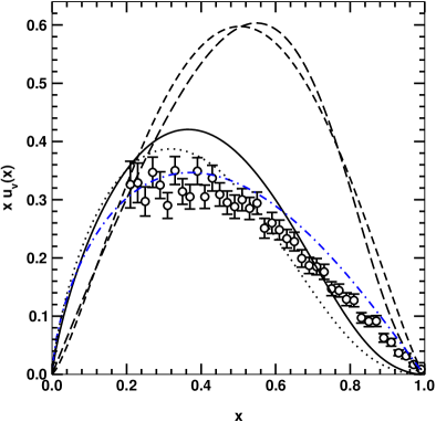
FIG. 3.: Dashed line: $xu_{v}(x;q_{0})$; Short-dashed line: fit of Eqs. (81) and (82); Solid line: the evolved distribution, $xu_{v}(x;q=2\,{\rm GeV})$; Dotted line: $xu_{v}(x;q=4.05\,{\rm GeV})$, evolved with a $4$-flavour value of $\Lambda_{\rm QCD}=0.204\,$GeV; and Dot-dashed line: the phenomenological fit of Ref. [4]. The data are from Ref. [2], obtained with an invariant $\mu^{+}\mu^{-}$-mass $>$ $4.05\,$GeV and inferred from the differential pion-nucleon Drell-Yan cross section using simple distribution parametrisations of the type in Eq. (81). This data was part of the set employed in the fit of Ref. [4]. The fits of Eqs. (84) and (85) are not depicted: they are almost indistinguishable from our calculated curves.

we obtain at $q=2\,$GeV

$$\begin{array}[]{l|lll}&\langle x\rangle_{q}&\langle x^{2}\rangle_{q}&\langle x^{3}\rangle_{q}\\ \hline\cr{\rm Calc.}&0.24&0.098&0.049\\ {\rm Fit}\cite[cite]{[\@@bibref{Number}{sutton}{}{}]}&0.24\pm 0.01&0.10\pm 0.01&0.058\pm 0.004\\ {\rm Latt.}\cite[cite]{[\@@bibref{Number}{lattice}{}{}]}&0.27\pm 0.01&0.11\pm 0.3&0.048\pm 0.020\end{array}$$ (80)

at which point the valence-quarks carry a momentum-fraction of $0.49$. At $q_{0}$, $\alpha_{s}/(2\pi)=0.13$: this is the combination that appears in the evolution equation. (NB. At $0.5\,q_{0}$, $\alpha_{s}/(2\pi)=0.68$.)

The original and evolved distributions are depicted in Fig. 3. The evident accentuation via evolution of the convex-up behaviour of the distribution near $x=1$ is characteristic of the renormalisation group equations, which populate the sea-quark distribution at small-$x$ at the expense of large-$x$ valence-quarks.

A fit to $x\,u_{v}(x;q)$, adequate for the rapid estimation of moments, is provided by the simple data fitting form employed in Refs. [2, 4]:

$$x\,u_{v}^{\rm mom}(x;q)=x^{\alpha}\,(1-x)^{\beta}\,\frac{\Gamma(1+\alpha+\beta)}{\Gamma(\alpha)\,\Gamma(1+\beta)}\,,$$ (81)

with in our case

$$\begin{array}[]{c|lll}q\,({\rm GeV})&0.57&2.0&4.05\\ \hline\cr\alpha&1.34&0.92&0.84\\ \beta&1.31&1.80&1.98\;.\end{array}\\$$ (82)

The moments of $u_{v}^{\rm mom}(x;q)$ are given by

$$\langle x^{n}\rangle_{q}=\prod_{i=1}^{n}\,\frac{i+\alpha-1}{i+\alpha+\beta}\,.$$ (83)

We emphasise, as is evident in Fig. 3, that Eq. (81) is not a good pointwise approximation to our calculated form of $x\,u_{v}(x;q_{0})$ and, furthermore, Eq. (81) divided-by $x$ provides a very poor pointwise approximation to $u_{v}(x;q_{0})$ for $x<0.5$.

An alternative parametrisation has also been employed[44] in fitting data:

$$x\,u_{v}^{\rm cu}(x)=A_{u}\,x^{\eta_{1}}\,(1-x)^{\eta_{2}}\,(1-\epsilon_{u}\,\sqrt{x}+\gamma_{u}\,x)\,,$$ (84)

with $A_{u}$ fixed by Eq. (38). This, with the parameter values:

$$\begin{array}[]{c|rrl}q\,({\rm GeV})&0.57&2.0&4.05\\ \hline\cr A_{u}&11.24&4.25&3.56\\ \eta_{1}&1.43&0.97&0.89\\ \eta_{2}&1.90&2.43&2.61\\ \epsilon_{u}&2.44&1.82&1.62\\ \gamma_{u}&2.54&2.46&2.30\;,\end{array}\\$$ (85)

provides a pointwise accurate interpolation of the calculated forms of $x\,u_{v}(x)$ depicted in Fig. 3: on the scale of this figure, the fit and our calculation are barely distinguishable. Furthermore, for $x\geq 0.2$, $u_{v}^{\rm cu}(x;q_{0})$ obtained from Eq. (84) even provides a good pointwise approximation to $u_{v}(x;q_{0})$ in Fig. 2. The difference between Eqs. (81) and (84) is the improved capacity of the latter to accommodate convexity in the parton distributions, which is a signal feature of our calculation.

Particular regularisations of the Nambu–Jona-Lasinio model yield[8, 9] a distribution with the functional form $u_{v}^{\theta}(x;q_{0}^{\rm NJL})=\theta(x)\,\theta(1-x)$, which corresponds to valence-quarks carrying each and every fraction of the pion’s momentum with equal probability. That result is an artefact, arising from the representation of the pion bound state by a momentum-independent Bethe-Salpeter amplitude; i.e., from representing the pion as a point-particle, which is a necessary consequence of the model’s momentum-independent interaction. In this case, beginning at $q_{0}^{\rm NJL}=0.35$, for which $\alpha/(2\pi)=0.31$, $x\,u_{v}^{\theta}(x;q_{0}^{\rm NJL})$ evolved to $q=2\,$GeV is pointwise very well described by Eq. (81) with $\alpha=0.67$, $\beta=1.13$, cf. the values in Ref. [4]: $\alpha=0.64\pm 0.03$, $\beta=1.15\pm 0.02$.

We infer from this result and the discussion above that the fitting form in Eq. (81) is inadequate: it is continuously connected to a distribution that lacks dynamical content and is unable to represent that structure in the distributions which characterises dynamics. These observations yield insight into the efficacy of the updated fitting form[44] in Eq. (84).

V Epilogue

We calculated the valence-quark distribution in the pion using a Dyson-Schwinger equation (DSE) model that provides a good description of a wide range of hadron observables: Figs. 2 and 3 summarise our new results. The DSE model describes valence-quarks with an active mass $\check{M}=0.30\,$GeV at a resolving scale $q_{0}=0.54\,$GeV$\,=1/(0.37\,{\rm fm})$, and with this value of $q_{0}$ the evolution to values of the momentum scale relevant to contemporary experiments yields a distribution whose low moments agree with the values obtained in lattice simulations and from a phenomenological fit.

There is a pointwise difference between our calculated distribution and the form used hitherto in parametrising pion data, as evident in Fig. 3. That discrepancy can also be observed in related covariant calculations[7, 9, 12]. From the information currently available, its origin does not appear to lie in model details, and we note that any assumed fitting form with little or no convexity in the vicinity of $x=1$, which is adapted to a body of data at a given scale, $q_{0}^{2}$, will necessarily become convex-up under evolution to an higher scale, $q^{2}>q_{0}^{2}$. Part or all of this discrepancy may therefore be attributable to the restricted function space used thus far in parametrising pion data. That possibility is supported by the capacity of an updated fitting form, used for the proton, to accommodate the structure evident in our calculations. However, we cannot rule out the possibility that the discrepancy may point to an as yet overlooked shortcoming in the application of models to the calculation of distribution functions.

Our calculation is a prototype. It can be improved; e.g., by using direct numerical solutions of the quark-DSE and meson Bethe-Salpeter equations, as in recent calculations of the light-meson electromagnetic form factors[39], and/or incorporating sea-quark contributions at the soft-scale, $q_{0}$. It can also be extended to more robust “targets,” such as the nucleon, using models like those of Refs. [23, 45].

REFERENCES

- [1] J. Badier et al. [NA3 Collaboration], Z. Phys. C 18, 281 (1983); B. Betev et al. [NA10 Collaboration], Z. Phys. C 28, 15 (1985).
- [2] J.S. Conway et al., Phys. Rev. D39, 92 (1989).
- [3] P. Aurenche, R. Baier, M. Fontannaz, M.N. Kienzle-Focacci and M. Werlen, Phys. Lett. B 233, 517 (1989).
- [4] P.J. Sutton, A.D. Martin, R.G. Roberts and W.J. Stirling, Phys. Rev. D 45, 2349 (1992).
- [5] C. Adloff et al. [H1 Collaboration], Eur. Phys. J. C 6, 587 (1999).
- [6] C. Best et al., Phys. Rev. D 56, 2743 (1997).
- [7] T. Shigetani, K. Suzuki and H. Toki, Phys. Lett. B 308, 383 (1993).
- [8] R.M. Davidson and E. Ruiz Arriola, Phys. Lett. B 348, 163 (1995); H. Weigel, E. Ruiz Arriola and L. Gamberg, Nucl. Phys. B560, 383 (1999).
- [9] W. Bentz, T. Hama, T. Matsuki and K. Yazaki, Nucl. Phys. A 651, 143 (1999).
- [10] A. Szczepaniak, C. Ji and S.R. Cotanch, Phys. Rev. D 49, 3466 (1994); T. Frederico and G.A. Miller, Phys. Rev. D 50, 210 (1994).
- [11] C.M. Shakin and W. Sun, Phys. Rev. C 51, 2171 (1995).
- [12] A.E. Dorokhov and L. Tomio, Phys. Rev. D 62 (2000) 014016.
- [13] C.D. Roberts and A.G. Williams, Prog. Part. Nucl. Phys. 33, 477 (1994).
- [14] A. Bender, C.D. Roberts and L. von Smekal, Phys. Lett. B 380, 7 (1996).
- [15] P. Maris, C.D. Roberts and P.C. Tandy, Phys. Lett. B 420, 267 (1998).
- [16] P. Maris and C.D. Roberts, Phys. Rev. C 56, 3369 (1997).
- [17] C.D. Roberts, R.T. Cahill, M.E. Sevior and N. Iannella, Phys. Rev. D 49, 125 (1994).
- [18] P. Maris and C.D. Roberts, Phys. Rev. C 58, 3659 (1998).
- [19] P. Maris and P.C. Tandy, Phys. Rev. C 61, 45202 (2000).
- [20] C.D. Roberts and S.M. Schmidt, Prog. Part. Nucl. Phys. 45, S1 (2000).
- [21] R. Alkofer and L. von Smekal, “The infrared behavior of QCD Green’s functions: Confinement, dynamical symmetry breaking, and hadrons as relativistic bound states,” hep-ph/0007355.
- [22] J.C.R. Bloch, C.D. Roberts, S.M. Schmidt, A. Bender and M.R. Frank, Phys. Rev. C 60, 062201 (1999); J.C.R. Bloch, C.D. Roberts and S.M. Schmidt, Phys. Rev. C 61, 065207 (2000).
- [23] M.B. Hecht, C.D. Roberts and S.M. Schmidt, “DSE Hadron Phenomenology,” nucl-th/0005067, to appear in the Proceedings of the Workshop on Light-Cone QCD and Nonperturbative Hadron Physics, Adelaide, Australia, 13-22 Dec 1999.
- [24] J.I. Skullerud and A.G. Williams, “Quark propagator in Landau gauge,” hep-lat/0007028.
- [25] P.V. Landshoff, J.C. Polkinghorne and R.D. Short, Nucl. Phys. B 28, 225 (1971).
- [26] Particle Data Group (D.E. Groom et al.), Eur. Phys. J. C 15, 1 (2000).
- [27] J.T. Londergan, G.T. Carvey, G.Q. Liu, E.N. Rodionov and A.W. Thomas, Phys. Lett. B 340, 115 (1994).
- [28] C.J. Burden, C.D. Roberts and M.J. Thomson, Phys. Lett. B 371, 163 (1996).
- [29] M.A. Pichowsky and T.-S.H. Lee, Phys. Lett. B 379, 1 (1996); M.A. Pichowsky and T.-S.H. Lee, Phys. Rev. D 56, 1644 (1997); F.T. Hawes and M.A. Pichowsky, Phys. Rev. C 59, 1743 (1999).
- [30] M.A. Pichowsky, S. Walawalkar and S. Capstick, Phys. Rev. D 60, 054030 (1999).
- [31] M.A. Ivanov, Yu.L. Kalinovsky and C.D. Roberts, Phys. Rev. D 60, 034018 (1999).
- [32] C.D. Roberts, “Continuum strong QCD: Confinement and dynamical chiral symmetry breaking,” nucl-th/0007054, a contribution to the Research Programme on Confinement at the Erwin Schrödinger Institute, Vienna, Austria, 5/May - 17/Jul/2000.
- [33] P. Maris and C.D. Roberts, “QCD bound states and their response to extremes of temperature and density,” in Proc. of the Workshop on Nonperturbative Methods in Quantum Field Theory, edited by A.W. Schreiber, A.G. Williams and A.W. Thomas (World Scientific, Singapore, 1998) pp. 132-151.
- [34] C.D. Roberts, Nucl. Phys. A 605, 475 (1996).
- [35] A. Bashir, A. Kizilersu and M.R. Pennington, Phys. Rev. D 57, 1242 (1998); and references therein.
- [36] J.S. Ball and T. Chiu, Phys. Rev. D 22, 2542 (1980).
- [37] M. Bando, M. Harada and T. Kugo, Prog. Theor. Phys. 91, 927 (1994); D. Kekez and D. Klabučar, Phys. Lett. B 457, 359 (1999); C.D. Roberts, Fizika B 8, 285 (1999); P.C. Tandy, ibid 295; B. Bistrovic and D. Klabučar, Phys. Lett. B 478, 127 (2000).
- [38] P. Maris and P.C. Tandy, Phys. Rev. C 60, 055214 (1999).
- [39] P. Maris and P.C. Tandy, Phys. Rev. C 62, 055204 (2000).
- [40] D.B. Leinweber, Annals Phys. 254, 328 (1997).
- [41] S.R. Amendolia et al. [NA7 Collaboration], Nucl. Phys. B 277, 168 (1986).
- [42] R. Alkofer, A. Bender and C.D. Roberts, Int. J. Mod. Phys. A 10, 3319 (1995).
- [43] K. Kusaka, G. Piller, A.W. Thomas and A.G. Williams, Phys. Rev. D 55, 5299 (1997).
- [44] A.D. Martin, W.J. Stirling and R.G. Roberts, Phys. Rev. D 50, 6734 (1994).
- [45] M. Oettel, R. Alkofer and L. von Smekal, Eur. Phys. J. A 8, 553 (2000).