Ghost-gluon running coupling, power corrections and the determination of $\Lambda_{\overline{\rm MS}}$

Abstract

We compute a formula including OPE power corrections to describe the running of a QCD coupling non-perturbatively defined through the ghost and gluon dressing functions. This turns out to be rather accurate. We propose the “plateau”-procedure to compute $\Lambda_{\overline{\rm MS}}$ from the lattice computation of the running coupling constant. We show a good agreement between the different methods which have been used to estimate $\Lambda_{\overline{\rm MS}}^{N_{f}=0}$. We argue that $\Lambda_{\overline{\rm MS}}$ or the strong coupling constant computed with different lattice spacings may be used to estimate the lattice spacing ratio.

1 Introduction

Much work has been devoted in the last years to the study of the QCD running coupling constant determined from lattice simulations, as well in its perturbative regime [1, 2, 3, 4, 5, 6, 7, 8, 9] as in the deep infrared domain [10]. The two main approaches to obtain the running coupling in terms of the renormalization momentum were either an application of the Schrödinger functional method with special boundary conditions or the confrontation of the behaviour with respect to the renormalization scale of 2-gluon and 3-gluon Green functions with the corresponding perturbative predictions. The latter Green’s functions approach also revealed a dimension-two non-zero gluon condensate in the landau gauge. Much work has been also done to investigate its phenomenological implications in the gauge-invariant world [11]. In a very recent work [9], the Green’s function approach to estimate $\Lambda_{\overline{\rm MS}}$ has been pursued by exploiting a non-perturbative definition of the coupling derived from the ghost-gluon vertex and computed over a large momentum window in the perturbative regime. Much of this work was based on the analysis of quenched lattice simulations and led to the determination of $\Lambda_{\overline{\rm MS}}$ in pure Yang-Mills ($N_{f}=0$). Works on unquenched lattice configurations ($N_{f}=2$) started some time ago [12] and have been more actively pursued recently.

Many unquenched configurations are presently available and we are planing to apply what we have learned on pure Yang-Mills to gauge configurations with twisted $N_{f}=2$ [13]) and $N_{f}=2+1+1$ dynamical quarks. Thus, a very realistic estimate of $\Lambda_{\overline{\rm MS}}$, directly comparable with experimental determinations, will become an immediate possibility. With the latter remarks in mind, we pay attention in this paper to study the above-mentioned non-perturbative coupling derived from the ghost-gluon vertex for being applied to the analysis of lattice data. We show in section 2 that, when the incoming ghost-momentum vanishes –and only in this case– this ghost-gluon vertex can be directly related to the bare gluon and ghost propagators; we then obtain a formula to describe its running including non-perturbative power corrections. We propose to confront this formula with lattice estimates of the coupling and argue that this constitutes an optimal method for the identification of $\Lambda_{\overline{\rm MS}}$ and of the gluon condensate. In particular, it benefits of two main advantages: to have only two-points function to deal with (much simpler to be managed and more precise than three-points ones) and that the precision could be improved by extending the analysis of lattice data over a very large momenta window. In section 3, we apply this procedure to previouly published lattice data for quenched simulations with a two-sided goal: (i) to check the method and (ii) to confirm the consistency of the picture we have acquired for the UV behaviour of Green functions in pure Yang-Mills. We finally conclude in section 4.

2 The ghost-gluon coupling

There is a large number of possibilities to define the QCD renormalized coupling constant, depending on the observable used to measure it and on the renormalization scheme. Actually, any observable which behaves, from the perturbative point of view, as $g$ provides a suitable definition for it. Among such quantities stand the 3-gluon and the ghost-gluon vertices, which have been widely used by the lattice community to get a direct knowledge of $\alpha_{s}$ from simulations. Of course an important criterion to choose among those definitions will be how easy it is to connect it to other commonly used definitions, specially the $\overline{MS}$ one, and to extract from it fundamental parameters like $\Lambda_{QCD}$.

A convenient class of renormalization schemes to work with on the lattice is made of the so-called “$MOM$” schemes which are defined through the requirement that a given scalar coefficient function of the Green’s function under consideration take its tree-level value in a specific kinematical situation given up to an overall “renormalization scale” . To make the point clearer we recall 2 schemes which we have used in previous works on $\alpha_{s}$:

• The symmetric 3-gluon scheme in which one uses the 3-gluon vertex $\Gamma_{\mu\nu\rho}(p_{1},p_{2},p_{3})$ with $p_{1}^{2}=p_{2}^{2}=p_{3}^{2}=\mu^{2}$

• The asymmetric 3-gluon scheme ($\widetilde{MOM}$) in which the 3-gluon vertex $\Gamma_{\mu\nu\rho}(p_{1},p_{2},p_{3})$ is used with $p_{1}^{2}=p_{2}^{2}=\mu^{2},\,p_{3}^{2}=0$

In the present note we shall apply a specific $MOM$-type renormalization scheme defined by fixing the (ghost and gluon) propagators and the ghost-gluon vertex at the renormalization point. Let us start by writing the ghost and gluon propagators in Landau gauge as follows,

$$\left(G^{(2)}\right)_{\mu\nu}^{ab}(p^{2},\Lambda) = \frac{G(p^{2},\Lambda)}{p^{2}}\ \delta_{ab}\left(\delta_{\mu\nu}-\frac{p_{\mu}p_{\nu}}{p^{2}}\right)\ ,$$

$$\left(F^{(2)}\right)^{a,b}(p^{2},\Lambda) = -\delta_{ab}\ \frac{F(p^{2},\Lambda)}{p^{2}}\ ;$$ (1)

$\Lambda$ being some regularisation parameter ($a^{-1}(\beta)$ if, for instance, we specialise to lattice regularisation). The renormalized dressing functions, $G_{R}$ and $F_{R}$ are defined through :

$$G_{R}(p^{2},\mu^{2})\ =\ \lim_{\Lambda\to\infty}Z_{3}^{-1}(\mu^{2},\Lambda)\ G(p^{2},\Lambda)$$

$$F_{R}(p^{2},\mu^{2})\ =\ \lim_{\Lambda\to\infty}\widetilde{Z}_{3}^{-1}(\mu^{2},\Lambda)\ F(p^{2},\Lambda)\ ,$$ (2)

with renormalization condition

$$G_{R}(\mu^{2},\mu^{2})=F_{R}(\mu^{2},\mu^{2})=1\ .$$ (3)

Now, we will consider the ghost-gluon vertex which could be non-perturbatively obtained through a three-point Green function, defined by two ghost and one gluon fields, with amputated legs after dividing by two ghost and one gluon propagators. This vertex can be written quite generally as:

$$\widetilde{\Gamma}^{abc}_{\nu}(-q,k;q-k)=\begin{picture}(100.0,25.0)(0.0,-3.0) \put(0.0,0.0){} \put(0.0,0.0){} \put(0.0,0.0){} \put(0.0,0.0){} \put(0.0,0.0){} \raise-10.0pt\hbox to0.0pt{\kern 12.5pt\makebox(0.0,0.0)[l]{k}\hss} \ignorespaces \raise-10.0pt\hbox to0.0pt{\kern 87.5pt\makebox(0.0,0.0)[r]{q}\hss} \ignorespaces \raise 20.0pt\hbox to0.0pt{\kern 60.0pt\makebox(0.0,0.0)[l]{q-k}\hss} \ignorespaces \end{picture}=ig_{0}f^{abc}\left(q_{\nu}H_{1}(q,k)+(q-k)_{\nu}H_{2}(q,k)\right)\ ,$$ (4)

where $q$ is the outgoing ghost momentum and $k$ the incoming one, and renormalized according to:

$$\widetilde{\Gamma}_{R}=\widetilde{Z}_{1}\Gamma.$$ (5)

The vertex $\Gamma_{\nu}$ involves two independent scalar functions. In the MOM renormalization procedure $\widetilde{Z}_{1}$ is fully determined by demanding that one specific combination of those two form factors (chosen at one’s will) be equal to its tree-level value for a specific kinematical configuration. We choose to apply MOM prescription for the scalar function $H_{1}+H_{2}$ that multiplies $q_{\nu}$ in eq. (4) and the renormalization condition reads

$$\left.(H^{R}_{1}(q,k)+H^{R}_{2}(q,k))\right|_{q^{2}=\mu^{2}}=\lim_{\Lambda\to\infty}\widetilde{Z}_{1}(\mu^{2},\Lambda)\left.(H_{1}(q,k;\Lambda)+H_{2}(q,k;\Lambda))\right|_{q^{2}=\mu^{2}}=1,$$ (6)

where we prescribe a kinematics for the substraction point such that the outgoing ghost momentum is evaluated at the renormalization scale, while the incoming one, $k$, depends on the choice of several possible configurations; for instance: $k^{2}=(q-k)^{2}=\mu^{2}$ (symmetric configuration) or $k=0,\ (q-k)^{2}=\mu^{2}$ (asymmetric-ghost configuration).

On the other hand, the fields involved in the non-perturbative definition of the vertex $\Gamma_{\nu}$ in eq. (4) can be directly renormalized by their renormalization constants, $Z_{3}$ and $\widetilde{Z}_{3}$, and the same MOM prescription applied to the scalar combination $H_{1}+H_{2}$ also implies:

$$g_{R}(\mu^{2}) = \lim_{\Lambda\to\infty}\ \widetilde{Z}_{3}(\mu^{2},\Lambda)Z_{3}^{1/2}(\mu^{2},\Lambda)g_{0}(\Lambda^{2})\left.\left(H_{1}(q,k;\Lambda)+H_{2}(q,k;\Lambda)\rule[0.0pt]{0.0pt}{14.22636pt}\right)\right|_{q^{2}\equiv\mu^{2}}$$ (7)

$$= \ \lim_{\Lambda\to\infty}g_{0}(\Lambda^{2})\ \frac{Z_{3}^{1/2}(\mu^{2},\Lambda^{2})\widetilde{Z}_{3}(\mu^{2},\Lambda^{2})}{\widetilde{Z}_{1}(\mu^{2},\Lambda^{2})}\ .$$

We combine both eq. (6) and the first-line equation of (7) to replace $H_{1}+H_{2}$ and obtain the second line that shows the well-known relationship $Z_{g}=(Z_{3}^{1/2}\widetilde{Z}_{3})^{-1}\widetilde{Z}_{1}$, where $g_{R}=Z_{g}^{-1}g_{0}$.

We turn now to the specific $MOM$-type renormalization scheme defined by a zero incoming ghost momentum. Since those kinematics are the ones (and the only ones) in which Taylor’s well known non-renormalization theorem (cf. ref [14]) is valid we shall refer to this scheme as to the $T$-scheme and the corresponding quantities will bear a $T$ subscript. Then, in eq (4), we set $k$ to $0$ and get

$$\widetilde{\Gamma}^{abc}_{\nu}(-q,0;q)=ig_{0}f^{abc}\left(H_{1}(q,0)+H_{2}(q,0)\right)\,q_{\nu}\ .$$ (8)

Now, Taylor’s theorem states that $H_{1}(q,0;\Lambda)+H_{2}(q,0;\Lambda)$ is equal to 1 in full QCD for any value of $q$. Therefore, the renormalization condition eq. (6) implies $\widetilde{Z}_{1}(\mu^{2})=1$ and then

$$\alpha_{T}(\mu^{2})\equiv\frac{g^{2}_{T}(\mu^{2})}{4\pi}=\ \lim_{\Lambda\to\infty}\frac{g_{0}^{2}(\Lambda^{2})}{4\pi}G(\mu^{2},\Lambda^{2})F^{2}(\mu^{2},\Lambda^{2})\ ;$$ (9)

where we also apply the renormalization condition for the propagators, eqs. (2,3), to replace the renormalization constants, $Z_{3}$ and $\widetilde{Z}_{3}$, by the bare dressing functions. The remarkable feature of eq. (9) is that it involves only $F$ and $G$ so that no measure of the ghost-gluon vertex is needed for the determination of the coupling constant.

Equation (9) has extensively been advocated and studied on the lattice (see for instance reference [15]) and used for a determination of $\Lambda_{QCD}$ in reference [9]. However it must be stressed that the $T$-scheme is the only one in which $\widetilde{Z_{1}}=1$. In any other scheme $\widetilde{Z_{1}}$ will be finite (since going from one scheme to any other one only involves an additional finite renormalization) but will keep a non trivial dependence on the scale, in particular for the symmetric scheme of reference [16] that has been computed at one loop in ref. [17]. In such cases one must in principle apply the general definition (7) of the coupling constant; nevertheless the form (9) is used quite often in this case (for a kinematical configuration other than T-scheme’s) also as an approximation, specially in relation with the study of Dyson-Schwinger equations.

We conclude this section by recalling that, in any scheme, the standard renormalization flow dictating the evolution with respect to the scale,

$$g^{2}_{R}(\mu^{2}) = g^{2}_{R}(\mu^{\prime 2})\ \left(\frac{\widetilde{Z}_{1}(\mu^{\prime 2})}{\widetilde{Z}_{1}(\mu^{2})}\right)^{2}F^{2}_{R}(\mu^{2},\mu^{\prime 2})G_{R}(\mu^{2},\mu^{\prime 2})\ ,$$ (10)

will be straightfowrdly obtained from the second line of eq. (7) and the propagators renormalization conditions in eqs. (2,3), where

$$\widetilde{Z}_{1}(\mu^{2})=\lim_{\Lambda\to\infty}\widetilde{Z}_{1}(\mu^{2},\Lambda^{2})$$ (11)

because of the Taylor’s non-renormalization theorem. Of course, eq. (10) reduces to

$$g^{2}_{T}(\mu^{2}) = g^{2}_{T}(\mu^{\prime 2})F^{2}_{R}(\mu^{2},\mu^{\prime 2})G_{R}(\mu^{2},\mu^{\prime 2})\ .$$ (12)

in the $T$-scheme.

2.1 Pure perturbation theory

In ref. [18], the three-loop perturbative substraction of all the three-vertices appearing in the QCD Lagrangian for kinematical configurations with one vanishing momentum has been done (in particular, the one involved in the definition of the coupling by eq. (9)). Different definitions of the coupling constant can be related in perturbation theory through relations like :

$$\alpha_{T}(\mu^{2})\ =\ \overline{\alpha}(\mu^{2})\ \left(1+\sum_{i=1}c_{i}\left(\frac{\overline{\alpha}(\mu^{2})}{4\pi}\right)^{i}\ \right)\ ;$$ (13)

on the other hand, since eq. (9) completely defines the running of the coupling, after properly deriving both its l.h.s. and r.h.s., one obtains

$$\frac{1}{\alpha_{T}(\mu^{2})}\ \frac{d\alpha_{T}(\mu^{2})}{d\overline{\alpha}} = \frac{1}{\beta_{\overline{\rm MS}}(\overline{\alpha})}\left(2\ \lim_{\Lambda\to\infty}\frac{d}{d\ln{\mu^{2}}}\ln F(\mu^{2},\Lambda)+\lim_{\Lambda\to\infty}\frac{d}{d\ln{\mu^{2}}}\ln G(\mu^{2},\Lambda)\right)$$ (14)

$$= \frac{2\widetilde{\gamma}(\overline{\alpha})+\gamma(\overline{\alpha})}{\beta_{\overline{\rm MS}}(\overline{\alpha})}\rule[14.22636pt]{0.0pt}{14.22636pt}\ \ ;$$

where

$$\beta_{\overline{\rm MS}}(\overline{\alpha})\ =\ \frac{d\overline{\alpha}}{d\ln{\mu^{2}}}\ =\ -4\pi\ \sum_{i=0}\overline{\beta}_{i}\left(\frac{\overline{\alpha}}{4\pi}\right)^{i+2}$$ (15)

is the standard $\beta$-function for the running coupling renormalized according to the usual $\overline{\rm MS}$ prescription, while

$$\widetilde{\gamma}(\overline{\alpha})\ =\ \lim_{\Lambda\to\infty}\frac{d\ln{\widetilde{Z}_{3,{\rm MOM}}(\mu^{2},\Lambda)}}{d\ln{\mu^{2}}}\ =\ \lim_{\Lambda\to\infty}\frac{d\ln{F(\mu^{2},\Lambda)}}{d\ln{\mu^{2}}}\ =\ -\sum_{i=0}\widetilde{\gamma}_{i}\left(\frac{\overline{\alpha}}{4\pi}\right)^{i+1}$$

$$\gamma(\overline{\alpha})\ =\ \lim_{\Lambda\to\infty}\frac{d\ln{Z_{3,{\rm MOM}}(\mu^{2},\Lambda)}}{d\ln{\mu^{2}}}\ =\ \lim_{\Lambda\to\infty}\frac{d\ln{G(\mu^{2},\Lambda)}}{d\ln{\mu^{2}}}\ =\ -\sum_{i=0}\gamma_{i}\left(\frac{\overline{\alpha}}{4\pi}\right)^{i+1}$$ (16)

are the anomalous dimensions for gluon and ghost propagators, both renormalized along MOM prescriptions (i.e., $G_{R}(\mu^{2},\mu^{2})=F_{R}(\mu^{2},\mu^{2})=1$), but expanded in terms of the $\overline{\rm MS}$ coupling $\overline{\alpha}$. The $\overline{\beta}_{i}$ coefficients in eq. (15) have been computed up to four loops in ref. [19], $\overline{\beta}_{0}$ and $\overline{\beta}_{1}$ being scheme-independent. Then, eqs.(13,15,2.1) can be applied to eq. (14) and one is led to deal with a coupled system of $n$ algebraic equations to compute the coefficients $c_{i}$ and determine $\alpha_{T}$ at $n$ loops. To summarize, the running of coupling constant $\alpha_{T}$, although formally defined from a three-point Green function, can be derived from the knowledge of the standard $\overline{\rm MS}$ $\beta$-function and only two-points functions for ghost and gluon. These two anomalous dimensions were computed in the $\overline{\rm MS}$ scheme at four loops in ref. [20] and were converted into the MOM scheme in ref. [21] for $N_{f}=0$ by applying

$$\gamma_{\Gamma,MOM}(\overline{\alpha}) = \lim_{\Lambda\rightarrow\infty}\frac{d\ln\left(Z_{\Gamma,{\rm MS}}(\mu^{2},\Lambda)\right)}{d\ln\mu^{2}}+\frac{d\ln\left(\Gamma_{R,\overline{\rm MS}}(\overline{\alpha})\right)}{d\ln\mu^{2}}$$ (17)

$$\equiv \gamma_{\Gamma,\overline{\rm MS}}(\overline{\alpha})+\frac{d\;\overline{\alpha}}{d\ln\mu^{2}}\ \frac{\partial}{\partial\;\overline{\alpha}}\ln\Gamma_{R,\overline{\rm MS}}(\overline{\alpha})\ ,$$

where $\Gamma$ stands generically for the two bare two-point dressing functions $F$ and $G$, $\Gamma_{R}$ for the renormalized ones  and $Z_{\Gamma}$ for the appropriate renormalization constant. Eq. (17) provides also the coefficients $\widetilde{\gamma}_{i}$ and $\gamma_{i}$ for any $N_{f}$ (see appendix A). Thus, one can solve the above mentioned coupled system of algebraic equations and obtain the coefficients $c_{i}$ in eq. (13), the first of those equations (the one stemming from matching the $1/\alpha$-terms in the 2 sides) resulting in the following constraint :

$$2\widetilde{\gamma}_{0}+\gamma_{0}=\overline{\beta}_{0}\ ,$$ (18)

which, in this context, results from eq. (9). The three first coefficients $c_{i}$ in Landau gauge, for instance, will be:

$$c_{1} = \frac{507-40N_{f}}{36}\ ,$$

$$c_{2} = \frac{76063}{144}-\frac{351}{8}\zeta(3)-\left(\frac{1913}{27}+\frac{4}{3}\zeta(3)\right)\ N_{f}+\frac{100}{91}N_{f}^{2}$$

$$c_{3} = \frac{42074947}{1728}-\frac{60675}{16}\zeta(3)-\frac{70245}{64}\zeta(5)-\left(\frac{769387}{162}-\frac{8362}{27}\zeta(3)-\frac{2320}{9}\zeta(5)\right)\ N_{f}$$ (19)

$$+ \left(\frac{199903}{972}+\frac{28}{9}\zeta(3)\right)\ N_{f}^{2}-\frac{1000}{729}\ N_{f}^{3}\ .$$

These three coefficients obviously define unambigously the running of $\alpha_{T}$ given in eq. (9) up to four-loops. In other words, one obtains for the $\beta$-function of $\alpha_{T}$,

$$\beta_{T}(\alpha_{T})\ =\ \frac{d\alpha_{T}}{d\ln{\mu^{2}}}\ =\ -4\pi\ \sum_{i=0}\widetilde{\beta}_{i}\left(\frac{\alpha_{T}}{4\pi}\right)^{i+2}\ ,$$ (20)

the following coefficients up to four-loops

$$\widetilde{\beta}_{0} = \overline{\beta}_{0}=11-\frac{2}{3}N_{f}$$

$$\widetilde{\beta}_{1} = \overline{\beta}_{1}=102-\frac{38}{3}N_{f}$$

$$\widetilde{\beta}_{2} = \overline{\beta}_{2}-\overline{\beta}_{1}c_{1}+\overline{\beta}_{0}(c_{2}-c_{1}^{2})$$

$$= 3040.48\ -\ 625.387\ N_{f}\ +\ 19.3833\ N_{f}^{2}$$

$$\widetilde{\beta}_{3} = \overline{\beta}_{3}-2\overline{\beta}_{2}c_{1}+\overline{\beta}_{1}c_{1}^{2}+\overline{\beta}_{0}(2\ c_{3}-6\ c_{2}c_{1}+4\ c_{1}^{3})$$ (21)

$$= 100541\ -\ 24423.3\ N_{f}\ +\ 1625.4\ N_{f}^{2}\ -\ 27.493\ N_{f}^{3}\ ,$$

These coefficients $\widetilde{\beta}_{i}$ are the same as the ones obtained in ref. [18] thanks to a direct application of the MOM prescription to the ghost-gluon coupling with vanishing incoming-ghost momentum, as it should be. As for the $\Lambda_{\rm QCD}$ parameters in the two schemes, they are related through

$$\frac{\Lambda_{\overline{\rm MS}}}{\Lambda_{T}}\ =\ e^{\displaystyle-\frac{c_{1}}{2\beta_{0}}}\ =\ e^{\displaystyle-\frac{507-40N_{f}}{792-48N_{f}}}\ .$$ (22)

Eq. (20) can be integrated and perturbatively inverted to obtain the following standard four-loop formula for the running coupling:

$$\begin{split}\alpha_{T}(\mu^{2})&=\frac{4\pi}{\beta_{0}t}\left(1-\frac{\beta_{1}}{\beta_{0}^{2}}\frac{\log(t)}{t}+\frac{\beta_{1}^{2}}{\beta_{0}^{4}}\frac{1}{t^{2}}\left(\left(\log(t)-\frac{1}{2}\right)^{2}+\frac{\widetilde{\beta}_{2}\beta_{0}}{\beta_{1}^{2}}-\frac{5}{4}\right)\right)\\ &+\frac{1}{(\beta_{0}t)^{4}}\left(\frac{\widetilde{\beta}_{3}}{2\beta_{0}}+\frac{1}{2}\left(\frac{\beta_{1}}{\beta_{0}}\right)^{3}\left(-2\log^{3}(t)+5\log^{2}(t)+\left(4-6\frac{\widetilde{\beta}_{2}\beta_{0}}{\beta_{1}^{2}}\right)\log(t)-1\right)\right)\\ &\mbox{\rm{with}}\ \ t=\ln{\frac{\mu^{2}}{\Lambda_{T}^{2}}}\ .\end{split}$$ (23)

As a last remark, applying the approximation $\widetilde{Z}_{1}=1$ for symmetric (ghost-gluon vertex renormalized at a symmetric momenta configuration) or soft-gluon (vertex renormalized at a vanishing-gluon momenta configuration) schemes implies that the same lattice data for the coupling, obtained through eq. (9), would be confronted to different perturbative formulae analogous to eq. (23) with $\beta$-function coefficients and $\Lambda_{\rm QCD}$ parameters apropriate for each scheme. Thus, the systematic deviation induced by applying this approximation to the determination of $\Lambda_{\overline{\rm MS}}$ from the confrontation of perturbation theory and lattice data, provided that $\beta_{0}$ and $\beta_{1}$ are scheme-independent, mainly results from the ratio of $\Lambda_{\rm QCD}$ to $\Lambda_{\overline{\rm MS}}$ in eq. (22). For instance in pure Yang-Mills, if one takes $N_{f}=0$ in eq. (22), it gives a ratio of 0.527 in T-scheme, while the same ratio for instance in symmetric and soft-gluon schemes is 0.463 (14 % of error) and 0.429 (23 % of error), respectively.

2.2 OPE power corrections

One of the goals of the present paper consists in obtaining a formula for the QCD running coupling that could be implemented in conjunction with lattice estimates to determine a “plateau” for $\Lambda_{\rm QCD}$ in terms of the momentum, as will be explained in the next section. In order to extend this “plateau” to energies as low as possible (of the order of 3 GeV) and to take full advantage of the lattice data in order to reduce the systematic uncertainties, it is mandatory to take into account the gauge-dependent dimension-two OPE power corrections (cf. [7, 8, 10, 23]) to $\alpha_{T}$.

The leading power contribution to the ghost propagator,

$$(F^{(2)})^{ab}(q^{2})=\int d^{4}xe^{iq\cdot x}\langle\ T\left(c^{a}(x)\overline{c^{b}}(0)\right)\ \rangle$$ (24)

can be computed using the operator product expansion [24] (OPE), as is done in ref. [22],

$$T\left(c^{a}(x)\overline{c^{b}}(0)\right)=\sum_{t}\left(c_{t}\right)^{ab}(x)\ O_{t}(0);$$ (25)

here $O_{t}$ is a local operator, regular when $x\to 0$, and the Wilson coefficient $c_{t}$ contains the short-distance singularity. Eq. (25) involves a full hierarchy of terms, ordered according to their mass-dimension, among which only ${\bf 1}$ and $:A_{\mu}^{a}A_{\nu}^{b}:$ contribute to eq. (24) in Landau gauge up to the order $1/q^{4}$. Then, using eq. (25) into eq. (24), we obtain:

$$(F^{(2)})^{ab}(q^{2}) = (c_{0})^{ab}(q^{2})\ +\ \left(c_{2}\right)^{ab\sigma\tau}_{st}(q^{2})\langle:A_{\sigma}^{s}(0)A_{\tau}^{t}(0):\rangle\ +\ \dots$$ (26)

$$= (F_{\rm pert}^{(2)})^{ab}(q^{2})\ +\ w^{ab}\ \frac{\langle A^{2}\rangle}{4(N_{C}^{2}-1)}\ +\ \dots$$

where

$$w^{ab}\ = \ \left(c_{2}\right)^{ab\sigma\tau}_{st}\delta^{st}g_{\sigma\tau}\ =\ \frac{1}{2}\ \delta^{st}g_{\sigma\tau}\frac{\int d^{4}xe^{iq\cdot x}\ \langle\widetilde{A}_{\tau^{\prime}}^{t^{\prime}}(0)\ T\left(c^{a}\overline{c^{b}}\right)\ \widetilde{A}_{\sigma^{\prime}}^{s^{\prime}}(0)\rangle_{\rm connected}}{{G^{(2)}}_{\sigma\sigma^{\prime}}^{ss^{\prime}}{G^{(2)}}_{\tau\tau^{\prime}}^{tt^{\prime}}}$$ (27)

$$= 2\times\rule[0.0pt]{0.0pt}{48.36958pt}\begin{picture}(150.0,25.0)(0.0,0.0) \put(0.0,0.0){} \put(0.0,0.0){} \put(0.0,0.0){} \put(0.0,0.0){} \put(0.0,0.0){} \put(0.0,0.0){} \put(0.0,0.0){} \put(0.0,0.0){} \put(0.0,0.0){} \end{picture},$$

and the SVZ factorisation [25] is invoked to compute the Wilson coefficients. Thus, one should compute the “sunset” diagram of the last line of eq. (27), that binds the ghost propagator to the gluon condensate (where the blue bubble means contracting the color and lorentz indices of the incoming legs with $1/2\delta_{st}\delta_{\sigma\tau}$) to obtain the leading non-perturbative contribution (of course, the first Wilson coefficient gives trivially the perturbative propagator).

Finally,

$$(F^{(2)}_{R})^{ab}(q^{2},\mu^{2})\ =\ (F^{(2)}_{R,{\rm pert}})^{ab}(q^{2},\mu^{2})\ \left(1+\frac{3}{q^{2}}\ \frac{g^{2}_{R}\langle A^{2}\rangle_{R,\mu^{2}}}{4(N_{C}^{2}-1)}\right)\ +\ {\cal O}\left(g^{4},q^{-4}\right)$$ (28)

where the $A^{2}$-condensate is renormalised at the subtraction point $q^{2}=\mu^{2}$, according to the MOM scheme definition, by imposing the tree-level value to the Wilson coefficient at the renormalization point. As far as we do not need to deal with the anomalous dimension of the $A^{2}$ operator, we can factorise the tree-level ghost propagator. The ghost dressing function is then written as:

$$F_{R}(q^{2},\mu^{2})\ =\ F_{R,{\rm pert}}(q^{2},\mu^{2})\ \left(1+\frac{3}{q^{2}}\frac{g^{2}_{R}\langle A^{2}\rangle_{R,\mu^{2}}}{4(N_{C}^{2}-1)}\right)\ ,$$ (29)

where the multiplicative correction to the purely perturbative $F_{R,{\rm pert}}$ is determined up to corrections of the order $1/q^{4}$ or $\ln{q/\mu}$ (the Wilson coefficient at the leading logarithm is computed in appendix B).

We can handle in the same way (see refs.[7, 8]) the OPE power correction to the gluon propagator and obtain

$$w_{\mu\nu}^{ab}\ = \begin{picture}(150.0,25.0)(0.0,0.0) \put(0.0,0.0){} \put(0.0,0.0){} \put(0.0,0.0){} \put(0.0,0.0){} \put(0.0,0.0){} \put(0.0,0.0){} \put(0.0,0.0){} \end{picture}+\ 2\times\rule[0.0pt]{0.0pt}{48.36958pt}\begin{picture}(150.0,25.0)(0.0,0.0) \put(0.0,0.0){} \put(0.0,0.0){} \put(0.0,0.0){} \put(0.0,0.0){} \put(0.0,0.0){} \put(0.0,0.0){} \put(0.0,0.0){} \put(0.0,0.0){} \put(0.0,0.0){} \end{picture}\$$ (30)

$$= \rule[14.22636pt]{0.0pt}{14.22636pt}\frac{3g^{2}}{q^{2}}\ (G_{\rm pert}^{(2)})_{\mu\nu}^{ab}.$$

Then, after renormalization, one gets

$$(G^{(2)}_{R})_{\mu\nu}^{ab}(q^{2},\mu^{2}) = (G_{R,\rm pert}^{(2)})_{\mu\nu}^{ab}(q^{2},\mu^{2})\ +\ \left(w_{\mu\nu}^{ab}\right)_{R,\mu^{2}}\ \frac{\langle A^{2}\rangle_{R,\mu^{2}}}{4(N_{C}^{2}-1)}\ +\ \dots$$ (31)

$$= \ (G^{(2)}_{R,{\rm pert}})_{\mu\nu}^{ab}(q^{2},\mu^{2})\ \left(1+\frac{3}{q^{2}}\ \frac{g^{2}_{R}\langle A^{2}\rangle_{R,\mu^{2}}}{4(N_{C}^{2}-1)}\right)\ +\ {\cal O}\left(g^{4},q^{-4}\right)\ \ .$$

and an appropriate projection gives for the gluon dressing function :

$$G_{R}(q^{2},\mu^{2})\ =\ G_{R,{\rm pert}}(q^{2},\mu^{2})\ \left(1+\frac{3}{q^{2}}\frac{g^{2}_{R}\langle A^{2}\rangle_{R,\mu^{2}}}{4(N_{C}^{2}-1)}\right)\ .$$ (32)

Finally, putting together the defining relation eq. (9) and the results eqs. (29,32) we get

$$\alpha_{T}(\mu^{2}) = \lim_{\Lambda\to\infty}\frac{g_{0}^{2}}{4\pi}F^{2}(\mu^{2},\Lambda)G(\mu^{2},\Lambda)$$ (33)

$$= \overbrace{\lim_{\Lambda\to\infty}\frac{g_{0}^{2}}{4\pi}F^{2}(q_{0}^{2},\Lambda)G(q_{0}^{2},\Lambda)}^{\displaystyle\alpha^{\rm pert}_{T}(q_{0}^{2})}\ F^{2}_{R}(\mu^{2},q_{0}^{2})\ G_{R}(\mu^{2},q_{0}^{2})$$

$$= \underbrace{\alpha^{\rm pert}_{T}(q_{0}^{2})F^{2}_{R,{\rm pert}}(\mu^{2},q_{0}^{2})\ G_{R,{\rm pert}}(\mu^{2},q_{0}^{2})}_{\displaystyle\alpha^{\rm pert}_{T}(\mu^{2})}\ \left(1+\frac{9}{\mu^{2}}\frac{g^{2}_{T}(q_{0}^{2})\langle A^{2}\rangle_{R,q_{0}^{2}}}{4(N_{C}^{2}-1)}\right)\ ,$$

where $q_{0}^{2}\gg\Lambda_{\rm QCD}$ is some perturbative scale and the $\beta$-function, and its coefficients in eq. (2.1), of course describe the running of the perturbative part of the evolution, $\alpha_{T}^{\rm pert}$.

The Wilson coefficient at the leading logarithm for the T-scheme MOM running coupling is presented in appendix B, where we also show that the inclusion of the logarithmic correction would induce no significant effect, provided that the coupling multiplying $A^{2}$ inside the bracket is taken to be renormalized also in T-scheme. Thus, for the sake of simplicity, eq. (33) will be applied for our analysis in the next section.

3 Data Analysis

In the following, we will first propose a “plateau”-procedure exploiting eq. (33) to get a reliable estimate of the $\Lambda_{\rm QCD}$-parameter from the lattice and we will apply it to previously published quenched lattice data [22, 21] as a check of the method.

3.1 The “plateau” method

The goal being to get a trustworthy estimate of the $\Lambda_{\overline{\rm MS}}$-parameter, one could attempt to do it by inverting the perturbative formula eq. (23) and using in the inverted formula the lattice estimates of the running coupling obtained by means of eq. (9) for as many lattice momenta as possible. Then, one should look for a “plateau” of $\Lambda_{\overline{\rm MS}}$ in terms of momenta in the high-energy perturbative regime (this was done with the coupling defined by the three-gluon vertex in [4, 5]). In the next subsection, fig. 2.(a) shows the estimates of $\Lambda_{\overline{\rm MS}}$ so calculated for the lattice data presented in ref. [22, 21] over $9\ \raise 1.29167pt\hbox{$<$\kern-7.5pt\raise-4.73611pt\hbox{$\sim$}}p^{2}\ \raise 1.29167pt\hbox{$<$\kern-7.5pt\raise-4.73611pt\hbox{$\sim$}}\ 33$ GeV².

However, in order to take advantage of the largest possible momenta window one can use instead eq. (33). In this way we shall hopefully be able to extend towards low momenta the region over which to look for the best possible values of the gluon condensate and of $\Lambda_{\overline{\rm MS}}$ . In other words, one requires the best-fit to a constant of

$$(x_{i},y_{i}) \equiv \left(p^{2}_{i},\Lambda(\alpha_{i})\right)\ ,$$

$${\rm with:}\ \ \ \ \ \alpha_{i} = \frac{\alpha_{\rm Latt}(p^{2}_{i})}{\displaystyle 1+\frac{c}{p^{2}_{i}}}\ ;$$ (34)

where $\Lambda(\alpha)$ is obtained by inverting the perturbative four-loop formula, eq. (23), and $c$ results from the best-fit (it appeared written in terms of the gluon condensate in eq. (33) ). Of course, $\Lambda(\alpha)$ reaches a “plateau” (if it does) behaving in terms of the momentum as a constant that we will take as our estimate of $\Lambda_{\overline{\rm MS}}$.

3.2 Applying the method

The lattice data that we will exploit here to check the method we have explained above were previously presented in ref. [21]. We refer to this work for all the details concerning the lattice implementation: algorithms, action, Faddeev-Popov operator inversion, etc.

The parameters of the whole set of simulations are described in table 1

$\beta$	Volume	$a^{-1}$ (GeV)	Number of confs.
$6.0$	$16^{4}$	$1.96$	$1000$
$6.0$	$24^{4}$	$1.96$	$500$
$6.2$	$24^{4}$	$2.75$	$500$
$6.4$	$32^{4}$	$3.66$	$250$

Table 1: Run parameters of the exploited data [21].

3.2.1 The scaling from different lattices

It should first be noted that the scaling of eq. (9) from the several lattices we use is indeed satisfactory. The prescription of taking the infinite cut-off limit in eq. (9) means in practice to have the lattice artifacts under control. This is in fact the case for UV ones. In particular, the hypercubic artifacts behaving as ${\cal O}(a^{k}\sum p_{i}^{k})$ for the lattice propagators we analyze were cured, as explained in [21], by exploiting the $H_{4}$-symmetry.

As an indirect way of testing that scaling, we consider all the lattice propagators as functions of the momentum measured in lattice units, (i.e. with dimensionless momenta $p_{\rm Lat}=a(\beta)p$, where $a(\beta)$ is the lattice spacing in physical units at the particular bare lattice coupling $g_{0}^{2}=6/\beta$), and determine the ratios of $a(\beta)$’s for the scaling to work. Then, still working in lattice units, the best-fit parameters to be obtained by applying the “plateau”-method will be $a(\beta)\,\Lambda_{\overline{\rm MS}}$ and $a^{2}(\beta)g^{2}_{T}\langle A^{2}\rangle_{R}$, and the ratio of those best-fit parameters for different lattices will provide the ratio of the corresponding lattice spacings.

$\beta$	Volume	$a(\beta)/a(6.2)$ (this work)	$a(\beta)/a(6.2)$ [1]	deviations (%)
$6.0$	$16^{4}$	$1.368$	$1.378$	0.7
$6.0$	$24^{4}$	$1.322$	$1.378$	4.1
$6.2$	$24^{4}$	$1$	$1$	0
$6.4$	$32^{4}$	$0.768$	$0.751$	2.2

Table 2: Comparison of lattice spacings ratios obtained by means of the scaling of eq. (9) as explained in the text and of the string-tension method.

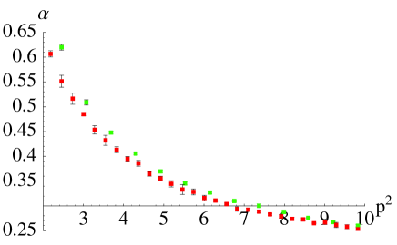
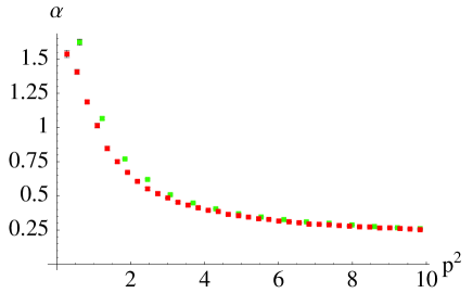
In tab. 2, the ratio of lattice spacings obtained by the standard string-tension method [1] are compared with those obtained as explained above. More precisely : (i) we first determine $\Lambda_{\overline{\rm MS}}a(6.2)$ and $a^{2}(6.2)g^{2}_{T}\langle A^{2}\rangle_{R}$ for the lattice data with $\beta=6.2$; (ii) then, for each new $\beta$, we determine $x=a(\beta)/a(6.2)$ in such a way that a “plateau” for $x\,a(6.2)\,\Lambda_{\overline{\rm MS}}$ is obtained with a gluon condensate given by $x^{2}\,a^{2}(6.2)\,g^{2}_{T}\langle A^{2}\rangle_{R}$. They agree very well, at least for the ratios computed for the three lattice simulations with roughly the same physical volume: $\beta=6.0(L=16=1.58$ fm), $\beta=6.2(L=24=1.72$ fm), $\beta=6.4(L=32=1.72$ fm). A slightly larger discrepancy ($\sim 4\%$) appears when comparing with data for the largest lattice ($\beta=6.0,L=24=2.37$ fm). We suspect that this is the manifestation of a finite-volume effect. Actually, if we compare the two simulations at $\beta=6.0$ for different volumes (see fig. 1), such an effect can be seen, although it decreases as the physical momentum increases (and becomes in practice negligible at $p^{2}\sim 9$ GeV²).

Thus, one can conclude that the scaling of the coupling defined by eq. (9) for $p^{2}\raise 1.29167pt\hbox{$>$\kern-7.5pt\raise-4.73611pt\hbox{$\sim$}}9$ GeV² is very good. Conversely, this argument provides an alternative method to determine the lattice size for a simulation at a given $\beta$ in terms of the one known in physical units at any other one.

(a)	(b)

Figure 1: (a) Plot of $\alpha_{T}$ defined by eq. (9) in terms of the square of the renormalization momentum as computed from the two lattices at $\beta=6.0$ with different volumes: $V=16^{4}$ (green boxes) and $V=24^{4}$ (red boxes). (b) A zoom onto the high momenta region of the left plot.

3.2.2 Looking for the “plateau”

(a)

(b)

Figure 2: (a) Plot of $\Lambda_{\overline{\rm MS}}$ (in GeV) computed by the inversion of the four-loop perturbative formula eq. (23) as a function of the square of the momentum (in GeV²); the coupling is estimated from the lattice data through eq. (9). (b) Same as plot (a) except for applying the non-perturbative formula eq. (33) for the coupling and looking for the gluon condensate generating the best plateau over $9\ \raise 1.1625pt\hbox{$<$\kern-6.75pt\raise-4.2625pt\hbox{$\sim$}}\ p^{2}\ \raise 1.1625pt\hbox{$<$\kern-6.75pt\raise-4.2625pt\hbox{$\sim$}}\ 33$ GeV².

In fig. 2.(a), we show the estimates of $\Lambda_{\overline{\rm MS}}$ obtained when interpreting the lattice coupling computed by eq. (9) for any momentum $9\ \raise 1.29167pt\hbox{$<$\kern-7.5pt\raise-4.73611pt\hbox{$\sim$}}p^{2}\ \raise 1.29167pt\hbox{$<$\kern-7.5pt\raise-4.73611pt\hbox{$\sim$}}33$ GeV² in terms of the inverted four-loop perturbative formula for the coupling, eq. (23). The estimates systematically decrease as the squared momentum increases until around 22 GeV²; above this value, only a noisy pattern results. In fig. 2.(b), the same is plotted but inverting instead the non-perturbative formula including power corrections, eq. (33). The value of the gluon condensate has been determined by requiring a “plateau” to exist (as explained in the previous section) over the total momenta window.

(a)	(b)

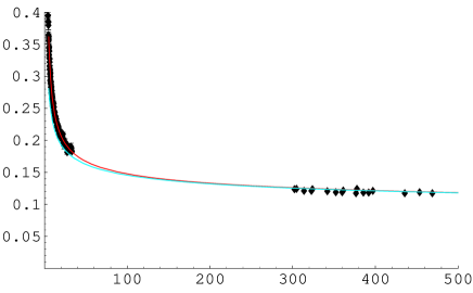
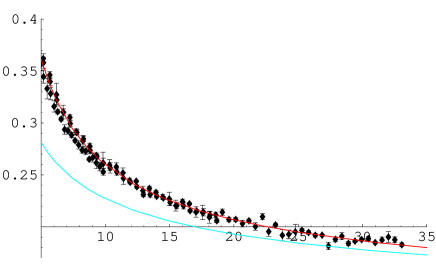
Figure 3: (a) Plot of $\alpha_{T}$ defined by eq. (9) in terms of the square of the renormalization momentum: the red solid line is computed with eq. (33) with $\Lambda_{\overline{\rm MS}}=224$ MeV, the blue one with eq. (23) for the same $\Lambda_{\overline{\rm MS}}$ and the data are obtained from the lattice data set-up in table 1. (b) The same but with some additional lattice estimates for the coupling at very high momenta (300–500 GeV²) taken from [9].

One should realize that, had we not taken into account the noisy ballpark of points above 22 GeV² and had we considered the perturbative regime as reached at that momentum, we would have got an estimate of $\Lambda_{\overline{\rm MS}}$ roughly 35-40 MeV above the one obtained from the non-perturbative formula. In other words, the non-perturbative analysis seems to indicate that the perturbative regime is far from being achieved at $p=5$ GeV. This is illustrated in figure 3 in which, adopting for $\Lambda_{\overline{\rm MS}}$ the value $224$ MeV which results from the non-perturbative analysis, we plot against the square of the renormalization momentum the coupling constant as computed by means of the non-perturbative formula (33) (red curve) and of the perturbative one (23) (blue curve). Displayed are also the lattice data, i.e. the values of $\alpha_{T}$ obtained from eq. (9). In figure 3.a the range in $\mu^{2}$ one sees that the non-perturbative approach provides a fairly good agreement with the data, the $\chi^{2}$ being 1.3 per degree of freedom. On the contrary there is a clear disagreement with the perturbative formula. Furthermore, one can extrapolate the value of the $\alpha_{T}$ up to very high momenta with eq. (33), $p^{2}\sim 300-500~{}\rm{GeV}^{2}$, where the purely perturbative eq. (23) and the non-perturbative eq. (33), both with the same $\Lambda_{\overline{\rm MS}}$, generate in practice the same results. The plot of fig. 3.(b) shows indeed that the curve for the coupling extrapolated in this way joins perfectly the lattice estimates at high momenta taken from [9]. Thus, the inclusion of the non-perturbative OPE power correction, eq. (33), to describe the running of the coupling eliminates effectively the observed systematic deviations for the estimates of $\Lambda_{\overline{\rm MS}}$ from the momenta window from 3 GeV to 5 GeV (fig. 2.(a) ) and essentially leads to the same estimate as was found from the perturbative regime at very high momentum.

(a)	(b)

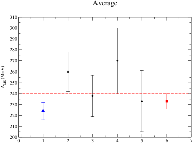
Figure 4: (a) The ellipsoid defined by $\chi^{2}(\Lambda_{\overline{\rm MS}},g^{2}_{T}\langle A^{2}\rangle_{R})=\chi^{2}_{\rm min}+1$. The y-axis is for $\Lambda_{\overline{\rm MS}}$ expressed in GeV and x-axis for $g^{2}_{T}\langle A^{2}\rangle_{R}$ in GeV². The small ellipsoid is obtained for a fitting window defined by $p^{2}>9$ GeV² and the larger is for $p^{2}>14$ GeV². (b) Comparison with previous estimates of $\Lambda_{\overline{\rm MS}}$ in pure Yang-Mills collected in tab. 3; the blue triangle stands for the estimate in this work and the red square for the average of the others. The 1-$\sigma$ error interval for the average (dashed red line) were estimated by treating the errors in tab. 3 as purely statistical ones.

Thus, we have been able to obtain simultaneous best-fit values for both the gluon condensate and $\Lambda_{\overline{\rm MS}}$. It is however manifest that they are correlated by their determination: the larger the gluon condensate is, the smaller the value of $\Lambda_{\overline{\rm MS}}$ has to be. In fig. 4, we plot the ellipsoid defined by  $\chi^{2}(\Lambda_{\overline{\rm MS}},g^{2}_{T}\langle A^{2}\rangle_{R})=\chi^{2}_{\rm min}+1$ for a fitting window defined by $p^{2}>8$ GeV² and for one restricted to $p^{2}>14$ GeV². It is seen that, neglecting other sources of errors like, for instance, the calibration of the lattices, but being conservative with the choice of the fitting window, one can conclude that our best-fit parameters incorporating only  statistical errors are:

$$\Lambda_{\overline{\rm MS}}^{Nf=0} = 224^{+8}_{-5}\ \rm{MeV}$$

$$g^{2}_{T}\langle A^{2}\rangle_{R} = 5.1^{+0.7}_{-1.1}\ \rm{GeV}^{2}\ .$$ (35)

These values are in very good agreement with the previous estimates from quenched lattice simulations of the three-gluon Green function [7, 8] or, in the case of $\Lambda_{\overline{\rm MS}}$, from the implementation of the Schrödinger functional method [2], although slightly larger than the one obtained by the ratio of ghost and gluon dressing functions [22] (see fig. 4.(b) and tab. 3). Concerning the gluon condensate estimate only, it is worth pointing that it can be computed at the renormalization momentum $\mu^{2}=100$ GeV² (see tab. 3) and it also agrees very well with the estimate from the analysis of the quark propagator vector part, $Z_{\psi}$, that gives: $\sqrt{\langle A^{2}\rangle_{R,\mu=10\ \rm{GeV}}}=1.76(8)$ GeV [26].

	$F^{2}G$ (this work)	Asym. 3-g [8]	Sym. 3-g [8]	$F/G$ [22]	[2]
$\Lambda_{\overline{\rm MS}}$ (MeV)	224${}^{+8}_{-5}$	260(18)	233(28)	270(30)	238(19)
$\sqrt{\langle A^{2}\rangle_{R,\mu}}$ (GeV)	1.64(17)	2.3(6)	1.9(3)	1.3(4)	–

Table 3: Comparison of estimates of $\Lambda_{\overline{\rm MS}}$ obtained from the analysis of the ghost-gluon vertex in this work (first column), the asymmetric 3-gluon vertex (second), the symmetric 3-gluon vertex (third), the ratio of gluon and ghost dressing functions (fourth) and with the Schrödinger functional method (last). The gluon condensate $\langle A^{2}\rangle_{R,\mu}$ has been obtained at the renormalization momentum $\mu=10$ GeV, for the sake of comparison with the other estimates, from eq. (3.2.2) by applying $g^{2}(\mu^{2}=100\ \rm{GeV}^{2})/4\pi=0.15$.

As a final remark, had we taken into account the leading-logarithm behaviour of the Wilson coefficient for the running coupling (applied eq. (44)) instead of eq. (33) ), the parameters so fitted would not significantly differ from those in eq. (3.2.2): we estimate a difference of $\sim 4\%$ in the determination of $g^{2}_{T}\langle A^{2}\rangle_{R}$ and less than $0.5\%$ in that of $\Lambda_{\overline{\rm MS}}$.

4 Conclusions

In the present paper we reconsider in some detail the determination of $\Lambda_{\overline{\rm MS}}$ from gluon and ghost Green functions using the MOM scheme. We stick here to the quenched case, or rather to the pure Yang-Mills $SU(3)$ theory, having of course in mind to apply what we learn also to the unquenched situation.

4.1 ghost-gluon vertex

We give some details about the proper renormalisation of the ghost-gluon vertex in the MOM scheme mainly because we realised that there is some carelessness in literature. An obvious remark is that applying MOM to a vertex function needs to specify the kinematics of the renormalisation point. Renormalising at the scale $\mu$ may be performed in the symmetric case, with the three momenta at the renormalisation scale ($p^{2}=\mu^{2}$) or in the soft gluon limite ($p_{gluon}=0,p^{2}_{ghost}=\mu^{2}$), or with a vanishing incoming ghost momentum, etc. The latter case is the one in which Taylor’s theorem applies which leads to $\widetilde{Z}_{1}=1$. We present in section 2.1 an alternative derivation of the perturbative renormalisation of the coupling constant in the latter scheme, defined by eq.  eq. (9), in agreement with the result by Chetyrkin [18]. The other kinematics lead to a finite but non trivial $\widetilde{Z}_{1}=1+O(\alpha^{2})$. This difference has been often overlooked, presumably because it is assumed to be small. However, as we have shown in section 2.1, applying $\widetilde{Z}_{1}=1$ to the symmetric case leads to a 14 % systematic error on $\Lambda_{\overline{\rm MS}}$ while it gives 23 % when applied to the soft gluon limit.

4.2 The $\Lambda_{\overline{MS}}$ plateau

$\Lambda_{\overline{\rm MS}}$ is a constant independent on the scale $\mu$. Inverting the perturbative expansion of the coupling constant one can invert eq. eq. (23) leading for each $\mu$ to $\Lambda_{\overline{\rm MS}}(\mu^{2})$ from $\alpha_{T}(\mu^{2})$ . If we were in a perturbative region of $\mu$ $\Lambda_{\overline{\rm MS}}(\mu^{2})$ should not depend on $\mu$ up to statistical errors. One should see a nice ”plateau”. Fig. 2.(a) shows that this is far from being the case up to $\mu^{2}=30\,{\mathrm{G}eV}^{2}$. We have since long advocated that there is a sizeable non-perturbative contribution from the vev of the unique (in Landau gauge) dimension 2 operator $\langle A^{2}\rangle$. We propose to fit this condensate by adjusting the resulting $\Lambda_{\overline{\rm MS}}$ to a “plateau”. This is successfully achieved, see fig. 2.(b). Since we scan a large window in the scale $\mu$ we believe that we are in a position to claim that we indeed see a non-perturbative $O(1/\mu^{2})$ contribution rather than the effect of logarithmically behaved higher orders in perturbation theory ($O(\alpha^{5})$).

4.3 Comparison of different estimates of $\Lambda_{\overline{MS}}$

We have performed a comparison of different estimates of $\Lambda_{\overline{\rm MS}}$ and $\langle A^{2}\rangle$ in the pure Yang-Mills theory using the coupling constant defined in eq. (9), the MOM coupling constant from symmetric three gluon vertex function, the MOM coupling constant from the three gluon vertex function with one vanishing momentum and from the ghost to gluon propagator ratio, and also with the estimate of $\Lambda_{\overline{\rm MS}}$ from the Schrödinger functional approach. The result is reported in table 3 and fig. 4.(b). The agreement is quite satisfactory. Fig 3.(b) shows also a good agreement of our fit from $\alpha_{T}(\mu^{2})$ with very large $\mu$ measurements from [9]. Notice also that $\Lambda_{\overline{\rm MS}}$ from $\alpha_{T}(\mu^{2})$ has the smallest statistical errors due to the fact that it relies only on propagator, not on noisier three point Green functions.

This opens a possibility of using the matching of $\Lambda_{\overline{\rm MS}}$ as computed from different lattices in order to fit the lattice spacing ratio. One might also match directly $\alpha_{T}(\mu^{2})$ from different lattices, a procedure which is not constrained to large scales and does not need to estimate the $\langle A^{2}\rangle$ condensate. In fact from eq. (9) we get directly a quantity which should be independant of the lattice spacing at the same $\mu$ in physical units, up to $O(1/a^{2})$ artifacts. This method is complementary to the use of Sommer’s parameter $r_{0}$ [27] and it also only depends on gauge fields.

Appendix A Appendix: ghost and gluon propagators anomalous dimension in MOM

The ghost and gluon anomalous dimension can be computed in MOM scheme by applying eq. (17) with the results obtained in ${\overline{\rm MS}}$ for the radiative corrections of all the relevant Green functions [18, 20]. Thus, one obtains for the coefficients defined in eq. (2.1) :

$$\widetilde{\gamma}_{0} = \frac{9}{4}$$

$$\widetilde{\gamma}_{1} = \frac{813}{16}-\frac{13N_{f}}{4}$$

$$\widetilde{\gamma}_{2} = \frac{157303}{64}-\frac{14909N_{f}}{48}+\frac{125N_{f}^{2}}{18}-\frac{5697\zeta(3)}{32}-\frac{21}{4}N_{f}\zeta(3)$$

$$\widetilde{\gamma}_{3} = \frac{219384137}{1536}-\frac{30925009N_{f}}{1152}+\frac{288155N_{f}^{2}}{216}-\frac{2705N_{f}^{3}}{162}-\frac{9207729\zeta(3)}{512}$$ (36)

$$+\frac{132749}{96}N_{f}\zeta(3)-\frac{19}{2}N_{f}^{2}\zeta(3)-\frac{221535\zeta(5)}{32}+\frac{15175}{16}N_{f}\zeta(5)$$

$$\gamma_{0} = \frac{13}{2}-\frac{2N_{f}}{3}$$

$$\gamma_{1} = \frac{3727}{24}-\frac{250\ N_{f}}{9}+\frac{20\ N_{f}^{2}}{27}$$

$$\gamma_{2} = \frac{2127823}{288}-\frac{9747\ \zeta(3)}{16}+N_{f}\left(-\frac{5210}{3}+\frac{119\zeta(3)}{3}\right)$$

$$+N_{f}^{2}\left(\frac{1681}{18}+\frac{16\ \zeta(3)}{9}\right)-\frac{200\ N_{f}^{3}}{243}$$

$$\gamma_{3} = \frac{3011547563}{6912}-\frac{18987543\zeta(3)}{256}-\frac{1431945\zeta(5)}{64}$$ (37)

$$+N_{f}\left(-\frac{221198219}{1728}+\frac{2897113\zeta(3)}{216}+\frac{845275\zeta(5)}{96}\right)$$

$$+N_{f}^{2}\left(\frac{6816713}{648}-\frac{60427\zeta(3)}{162}-\frac{4640\zeta(5)}{9}\right)$$

$$+N_{f}^{3}\left(-\frac{373823}{1458}-\frac{88\zeta(3)}{27}\right)+\frac{2000N_{f}^{4}}{2187}$$

These coefficients appear for the expansion, given by eq. (17), of the MOM-renormalized ghost and gluon anomalous dimension in terms of the $\overline{\rm MS}$-coupling. However, provided that the $\beta$-function for any other renormalization scheme is known, it can be applied to replace $\alpha_{\overline{\rm MS}}$ in eq. (2.1) by the coupling in that scheme.

Appendix B Appendix: Wilson coefficients at leading logarithms

The purpose of this appendix is to present up to leading logarithms the subleading Wilson coefficients in eqs. (29,32) and, in view of checking the validity of neglecting those logarithms, estimate their impact on the momenta window we use for our fits. Following [8], let us write

$$G_{R}(q^{2},\mu^{2}) = c_{0}\left(\frac{q^{2}}{\mu^{2}},\alpha(\mu^{2})\right)+c_{2}\left(\frac{q^{2}}{\mu^{2}},\alpha(\mu^{2})\right)\ \frac{\langle A^{2}_{R}\rangle_{\mu}}{4(N_{c}^{2}-1)q^{2}}$$

$$F_{R}(q^{2},\mu^{2}) = \widetilde{c}_{0}\left(\frac{q^{2}}{\mu^{2}},\alpha(\mu^{2})\right)+\widetilde{c}_{2}\left(\frac{q^{2}}{\mu^{2}},\alpha(\mu^{2})\right)\ \frac{\langle A^{2}_{R}\rangle_{\mu}}{4(N_{c}^{2}-1)q^{2}}\$$ (38)

for gluon and ghost propagators. Then, with the help of the appropriate renormalization constants one can rewrite eq. (B) in terms of bare quantities:

$$G(q^{2},\Lambda^{2}) = Z_{3}(\mu^{2},\Lambda^{2})\ c_{0}\left(\frac{q^{2}}{\mu^{2}},\alpha(\mu^{2})\right)$$ (39)

$$+ Z_{3}(\mu^{2},\Lambda^{2})Z_{A^{2}}^{-1}(\mu^{2},\Lambda^{2})\ c_{2}\left(\frac{q^{2}}{\mu^{2}},\alpha(\mu^{2})\right)\ \frac{\langle A^{2}\rangle}{4(N_{c}^{2}-1)q^{2}}\ ,$$

where $A^{2}_{R}=Z^{-1}_{A^{2}}A^{2}$. A totally analogous equation for the ghost dressing function $F(q^{2},\Lambda^{2})$, with $\widetilde{c}_{i}$ and $\widetilde{Z}_{3}$ in place of $c_{i}$ and $Z_{3}$. Now, as the $\mu$-dependence of both l.h.s. and r.h.s. of eq. (39) should match each other for any $q$, one can take the logarithmic derivative with respect to $\mu$ and infinite cut-off limit, term by term, on r.h.s. and obtains:

$$\gamma(\alpha(\mu^{2}))+\left\{\frac{\partial}{\partial\log\mu^{2}}+\beta(\alpha(\mu^{2}))\frac{\partial}{\partial\alpha}\right\}\ \ln c_{0}\left(\frac{q^{2}}{\mu^{2}},\alpha(\mu^{2})\right) = 0$$

$$-\gamma_{A^{2}}(\alpha(\mu^{2}))+\gamma(\alpha(\mu^{2}))+\left\{\frac{\partial}{\partial\log\mu^{2}}+\beta(\alpha(\mu^{2}))\frac{\partial}{\partial\alpha}\right\}\ \ln c_{2}\left(\frac{q^{2}}{\mu^{2}},\alpha(\mu^{2})\right) = 0\ ,$$ (40)

where $\gamma(\alpha(\mu^{2}))$ is the gluon propagator anomalous dimension defined in eq. (2.1) and

$$\gamma_{A^{2}}(\alpha(\mu^{2}))\ =\ \lim_{\Lambda\to\infty}\ \frac{d}{d\ln\mu^{2}}\ln Z_{A^{2}}(\mu^{2},\Lambda^{2})\ =\ -\gamma_{0}^{A^{2}}\ \frac{\alpha(\mu^{2})}{4\pi}\ +\dots$$ (41)

Both eqs. (B) can be finally combined to give:

$$\left\{-\gamma_{A^{2}}(\alpha(\mu^{2}))+\frac{\partial}{\partial\log\mu^{2}}+\beta(\alpha(\mu^{2}))\frac{\partial}{\partial\alpha}\right\}\ \frac{c_{2}\left(\frac{q^{2}}{\mu^{2}},\alpha(\mu^{2})\right)}{c_{0}\left(\frac{q^{2}}{\mu^{2}},\alpha(\mu^{2})\right)}\ =\ 0\ .$$ (42)

We can proceed in the same way for the ghost dressing function and derive analogous equations for the Wilson coefficients, $\widetilde{c}_{i}$, that differ from those for $c_{i}$ only because $\widetilde{\gamma}(\alpha(\mu^{2}))$ takes the place of $\gamma(\alpha(\mu^{2}))$. Thus, the combination $\widetilde{c}_{2}/\widetilde{c}_{0}$ obeys exactly the same eq. (42), above derived for $c_{2}/c_{0}$, that can be solved at the leading logarithm as explained in [8] to give:

$$\frac{c_{2}\left(\frac{q^{2}}{\mu^{2}},\alpha(\mu^{2})\right)}{c_{0}\left(\frac{q^{2}}{\mu^{2}},\alpha(\mu^{2})\right)}\ =\ \frac{\widetilde{c}_{2}\left(\frac{q^{2}}{\mu^{2}},\alpha(\mu^{2})\right)}{\widetilde{c}_{0}\left(\frac{q^{2}}{\mu^{2}},\alpha(\mu^{2})\right)}\ =\ 3g^{2}(q^{2})\ \left(\frac{g^{2}(q^{2})}{g^{2}(\mu^{2})}\right)^{-\gamma_{0}^{A^{2}}/\beta_{0}}\ .$$ (43)

The boundary condition comes from requiring eq. (B) to be equal to eq. (29) for the ghost and eq. (32) for the gluon at $\mu^{2}=q^{2}$. The coefficient $\gamma_{0}^{A^{2}}$ was computed to be 35/4 for the first time in [8]. Of course, eqs. (B) define not only the dependence of the Wilson coefficient on the renormalization momentum, $\mu^{2}$, but also that on the momentum scale $q^{2}$ because of standard dimensional arguments: the only dimensionless quantities are the ratio $q^{2}/\mu^{2}$ and $\alpha$. Then, putting all toghether, the non-perturbative formula for the running coupling at the leading logarithm is given by

$$\alpha_{T}(\mu^{2})\ =\ \alpha^{\rm pert}_{T}(\mu^{2})\ \left(1+\frac{9}{\mu^{2}}\left(\frac{\ln\frac{\mu^{2}}{\Lambda^{2}_{QCD}}}{\ln\frac{\mu_{0}^{2}}{\Lambda^{2}_{QCD}}}\right)^{-9/44}\frac{g^{2}_{T}(\mu_{0}^{2})\langle A^{2}\rangle_{R,\mu_{0}^{2}}}{4(N_{C}^{2}-1)}\right)\ ,$$ (44)

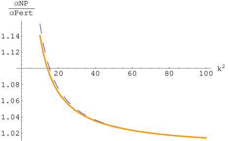
where the only correction to eq. (33) comes from the ratio of logarithms inside the bracket that, as can be seen in fig. 5, introduces no significant deviation.

Figure 5: $\alpha^{\rm NP}/\alpha^{\rm pert}$ in terms of the square of the momentum computed by using both eq. (44) (dashed blue) and eq. (33) (solid red).

References

• [1] G. S. Bali and K. Schilling, Phys. Rev.  D 47 (1993) 661 [arXiv:hep-lat/9208028].
• [2] M. Luscher, R. Sommer, P. Weisz and U. Wolff, Nucl. Phys.  B 413 (1994) 481; S. Capitani, M. Luscher, R. Sommer and H. Wittig [ALPHA Collaboration], Nucl. Phys.  B 544 (1999) 669 [arXiv:hep-lat/9810063].
• [3] G. M. de Divitiis, R. Frezzotti, M. Guagnelli and R. Petronzio, Nucl. Phys.  B 433 (1995) 390 [arXiv:hep-lat/9407028].
• [4] B. Alles, D. Henty, H. Panagopoulos, C. Parrinello, C. Pittori and D. G. Richards, Nucl. Phys.  B 502 (1997) 325 [arXiv:hep-lat/9605033].
• [5] P. Boucaud, J. P. Leroy, J. Micheli, O. Pene and C. Roiesnel, JHEP 9810 (1998) 017 [arXiv:hep-ph/9810322].
• [6] P. Boucaud et al., JHEP 0004 (2000) 006 [arXiv:hep-ph/0003020].
• [7] Ph. Boucaud, A. Le Yaouanc, J.P. Leroy, J. Micheli, O. Pène, J. Rodriguez-Quintero, Phys. Lett. B493 (2000) 315;
• [8] Ph. Boucaud,A. Le Yaouanc, J.P. Leroy, J. Micheli, O. Pène, J. Rodriguez-Quintero, Phys. Rev. D63 (2001) 114003; F. De Soto and J. Rodriguez-Quintero, Phys. Rev. D 64 (2001) 114003 ;
• [9] A. Sternbeck, K. Maltman, L. von Smekal, A. G. Williams, E. M. Ilgenfritz and M. Muller-Preussker, PoS LAT2007 (2007) 256 [arXiv:0710.2965 [hep-lat]].
• [10] P. Boucaud et al., Phys. Rev.  D 66 (2002) 034504; JHEP 0304 (2003) 005; Phys. Rev.  D 70 (2004) 114503.
• [11] F. V. Gubarev and V. I. Zakharov, Phys. Lett.  B 501 (2001) 28 [arXiv:hep-ph/0010096].
• [12] P. Boucaud, J. P. Leroy, H. Moutarde, J. Micheli, O. Pene, J. Rodriguez-Quintero and C. Roiesnel, JHEP 0201 (2002) 046 [arXiv:hep-ph/0107278].
• [13] Ph. Boucaud et al. [ETM collaboration], arXiv:0803.0224 [hep-lat].
• [14] J.  C.  Taylor, Nuclear Physics B33 (1971) 436
• [15] L. von Smekal, R. Alkofer and A. Hauck, Phys. Rev. Lett.  79 (1997) 3591 [arXiv:hep-ph/9705242].
• [16] K. G. Chetyrkin, K. G. and T. Seidensticker, Phys. Lett. B 495 (2000) 74 [arXiv:hep-ph/0008094].
• [17] Ph. Boucaud, J. P. Leroy, A. Le Yaouanc, A. Y. Lokhov, J. Micheli, O. Pene, J. Rodríguez Quintero and C. Roiesnel, hep-ph/0507104, 2005.
• [18] K. G. Chetyrkin and A. Retey, [arXiv:hep-ph/0007088].
• [19] T. van Ritbergen, J. A. M. Vermaseren and S. A. Larin, Phys. Lett. B 400 (1997) 379 [arXiv:hep-ph/9701390].
• [20] K. G. Chetyrkin, Nucl. Phys. B 710 (2005) 499 [arXiv:hep-ph/0405193];
• [21] Ph. Boucaud et al., Phys. Rev.  D 72 (2005) 114503 [arXiv:hep-lat/0506031].
• [22] Ph. Boucaud et al., JHEP 0601 (2006) 037 [arXiv:hep-lat/0507005]; Ph. Boucaud,A. Le Yaouanc, J.P. Leroy, J. Micheli, O. Pène, J. Rodriguez-Quintero, Phys. Rev. D63 (2001) 114003
• [23] D. Dudal, H. Verschelde and S. P. Sorella, Phys. Lett. B 555 (2003) 126 ; K. I. Kondo, Phys. Lett. B 572 (2003) 210 ; [arXiv:hep-th/0306195].
• [24] R. Wilson, Phys. Rev. 179 (1969) 1499.
• [25] M.A. Shifman, A.I. Vainshtein, V.I. Zakharov, Nucl. Phys. B147 (1979) 385,447,519; M.A. Shifman, A.I. Vainshtein, M.B. Voloshin, V.I. Zakharov, Phys. Lett. B77 (1978) 80;
• [26] Ph. Boucaud et al., Phys. Rev.  D 74 (2006) 034505 [arXiv:hep-lat/0504017].
• [27] R. Sommer, Nucl. Phys.  B 411 (1994) 839