Toward Resolved Simulations of Burning Fronts in Thermonuclear X-ray Bursts

Abstract

We discuss the challenges of modeling X-ray bursts in multi-dimensions, review the different calculations done to date, and discuss our new set of ongoing simulations. We also describe algorithmic improvements that may help in the future to offset some of the expense of these simulations, and describe what may be possible with exascale computing.

1 Introduction

X-ray bursts (XRBs) are fascinating astrophysical explosions. A neutron star accretes fuel from its binary companion, building up just a thin layer ($\sim 5$–$10$ m) before the immense gravitational acceleration at the neutron star surface compresses and heats the fuel to the point of thermonuclear runaway. A brief flash of X-rays follows, the accreted layer diffuses the heat produced from reactions, and the process repeats. We can observe multiple bursts from a single source, and the information their lightcurves encodes tells us about the underlying neutron star, and ultimately the nuclear equation of state. A challenging aspect of interpreting the lightcurves is understanding the radiation transport through the hot ash layers. In particular, the composition can affect the effective temperature, which in turn affects the radius we measure for the neutron star [1]. Convection in the burning layer can even bring ashes up to the photosphere which alters what we see [2]. Accurate measurements of neutron star radii from XRBs could greatly constrain the nuclear equation of state [3, 4]. Finally, brightness oscillations during the rising phase of the bursts and other features seen in lightcurves are interpreted as arising from the spreading of a hotspot across the neutron star—demonstrating that the burst begins in a localized region [5, 6]. See [7] for a recent review of XRBs.

Simulations of XRBs can help us to understand the observations, but many technical challenges remain. The primary difficulties are simply the range of length and timescales involved. At the largest lengthscale, the neutron star radius is 10 km and the Rossby lengthscale, where rotation and lateral pressure gradients balance, is $\sim 1$ km [8]. At the smallest scales, a conductive He flame has a thickness of 10s of centimeters [9] and the pressure scale height of the fuel layer is on the order of meters. To capture the rise timescale of the XRB, we would need to model seconds, but the flame itself is subsonic, so long timescale evolution is difficult.

Present and past simulations of XRBs employ a variety of approximations to get past these difficulties. The variety of approximations used enables a complementary picture of XRBs to be built up, and has greatly advanced our understanding of these systems. The breadth of simulations to date has been impressive. We summarize the different approaches below.

One-dimensional simulations, e.g. [10, 11], assume spherical symmetry and model the burst through the vertical column depth of fuel. These simulations can capture the luminosities and burst recurrence times well. They can utilize very large nuclear reaction networks and have been used to understand the nucleosynthesis and rp-process [12, 13, 14], as well as to understand how rate uncertainties can affect the outcomes of the bursts. Many successive bursts can be modeled and these simulations can show us the evolution of the ash layer with time. The approximation of 1D however means that we cannot learn about lateral variations across the neutron star, including flame spreading.

Global shallow water simulations [8] capture the large scale spreading of the burning front by using a very simple vertical structure. These simulations were instrumental in showing that the Coriolis force plays an important role in confining a spreading region and that the flame spreading can explain brightness oscillations during the rise of the burst lightcurve.

Our group and others have modeled the convection preceding the runaway using low Mach number hydrodynamic methods for pure helium bursts [15, 16] and mixed hydrogen/helium bursts [17] in 2D, as well as full 3D simulations of mixed bursts [18], and followed the development of turbulence. These simulations can give an understanding of the pre-burning front regime, including the strength and character of the turbulence, but cannot model large scale lateral variations because of the implicit assumptions built into the low Mach number model [19].

While detonations are computationally easier to model than flames (we largely get the speed through the jump conditions in the Riemann problem without resolving the structure), detonations require extreme conditions not found in XRBs [20, 21]. This means that calculations that want to capture the nucleosynthesis yields from spreading burning fronts in XRBs need to model a deflagration.

Flame spreading was first modeled in a series of calculations employing an algorithm from atmospheric science, where vertical hydrostatic equilibrium is enforced and wide-aspect ratio zones give a horizontal CFL number that is large enough to obtain long timescale evolution [22]. These calculations display key features of the propagation mechanism, namely a balance between hydrodynamics and the pure flame physics. The flame proceeds mainly via conduction, thus being a deflagration. The flame front, however, is not vertical but inclined, the angle with the horizontal being very small: $\theta\sim H/R_{\rm{Ro}}\sim 10^{-3}$. Here $H$ is the scale height and $R_{\rm{Ro}}$ is the Rossby radius. It is the hydrodynamical balance between the Coriolis force, gravity and pressure gradients that determines the Rossby radius and therefore the inclination angle of the flame front. The extended surface of the flame front is what leads to propagation speeds of order $10^{5}$ km/s, in good agreement with observations. Due to its dependence on the Coriolis force, the flame speed changes across the surface of the NS (being faster at the equator), leading to potentially detectable effects if the rise of the burst is observed with enough resolution [23]. We note that there may be preexisting turbulence ahead of the flame from simmering occurring there, and no calculations have considered the effects of the flame interacting with this turbulence, as we characterized in [18]. Flame-turbulence interactions have long been seen as a means to accelerate a flame in Type Ia supernovae, so future studies should look at turbulence in the layer. Capturing turbulence, of course, requires high resolution, so the ideas described here will be needed.

The NS systems exhibiting XRBs are expected to have magnetic fields in the range $10^{7}$–$10^{10}$ G. Inclusion of a vertical magnetic field proved to have a strong influence on the nature and the speed of flame propagation [24], due to the interaction between the Coriolis force and the magnetic tension, which further acts towards determining the inclination angle of the flame front.

A longstanding goal is to perform simulations where we resolve the flame structure, to allow us to accurately capture the nucleosynthesis, and watch it move across the neutron star surface. The results of these simulations will enable strict comparison to observations made with the new generation of X-ray telescopes such as eXTP and STROBE-X [25, 26, 27] which will offer high collecting area and time resolution. We show some in-progress calculations that are a step toward this, discuss their remaining approximations, and also discuss what new algorithmic techniques might be needed to realize this goal with the advent of exascale computing.

2 Resolved Flame Studies

We have begun a set of flame spreading calculations using the compressible hydrodynamics code Castro [28], part of the AMReX astrophysics suite [29]. Castro uses adaptive mesh refinement, supports a general equation of state and reaction networks, has a conservative gravity formulation [30], and is optimized to run on current supercomputers. All of our code base is open source and available on GitHub, and all of the solvers, problem setup, initial models, and analysis scripts for each of our science problems are distributed with the codes.

We setup a problem by creating a pair of 1D hydrostatic XRB models (hot and cool) representing the post- and pre-flame states and apply these laterally across the domain to setup a hot region at the left end of our domain in equilibrium with the cool model on the right. Thermal diffusion and nuclear reactions quickly produce a laterally propagating flame that begins to move through our domain. We resolve the diffusion scale, using a resolution of 10 cm, and use adaptive mesh refinement (two jumps of $4\times$) to keep a buffer of low density material at low resolution above the surface to allow for expansion. To make the lengthscales tractable, we rotate the neutron star at 2000 Hz—much faster than expected. This helps confine the spreading region to a more reasonable horizontal domain. Nevertheless, our simulation uses 12288 zones laterally, on the finest grid. We use the stellar conductivities from [9] and a 13-isotopic alpha-chain reaction network. To make the timescales easier, we boost the flame speed by a factor of 10 by scaling both the conductivity and energy generation rate by the same factor. This is an approximation we hope to relax in the near future.

Figure 1 shows the flame structure for an initial 2D run at 0.007 s. Vertical profiles at a few radial distances from the origin are shown for the same quantities in Figure 2. The burning layer is only about 10 m high. Underneath is ${}^{56}\mathrm{Ni}$, representative of the underlying neutron star, and above it is a very low density ($10^{-4}~{}\mathrm{g~{}cm^{-3}}$) buffer. Only a portion of the vertical extent is shown. The top panel shows the temperature structure. The initial perturbation reached to $2\times 10^{4}~{}\mathrm{cm}$, so at this point, the extent of the burnt region has nearly doubled. The flame structure is quite wide, since there are multiple burning stages beyond just helium to carbon, and this shows up in the composition. This is seen more clearly in the next panel which shows the mean molecular weight of the nuclei ($\bar{A}$). We see that the further behind the head of the flame we are, the heavier the ash nuclei. We also see the head of the flame appears lifted off of the base of the burning layer—unburned material underlies the spreading flame. This is reminiscent of the flame structure seen in the earlier simulations of [22]. The third panel shows the energy generation rate. It is strongest just above the neutron star surface, behind the flame. We again see that the head of the flame is detached from the base of the atmosphere, with the strongest burning at the head of the flame slightly higher up in the atmosphere. Finally, the bottom panel shows the velocity through the plane of the simulation—this is induced by the Coriolis force as the burning fluid expands and begins to spread laterally. A tight hurricane structure has setup as a result of the flame spreading. This is the geostrophic balance discussed in [8]. These calculations are ongoing and will be the subject of a detailed study in the near future.

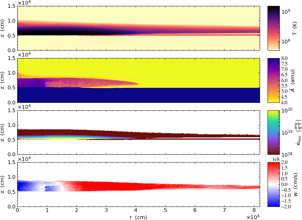
Figure 1: Helium flame spreading across the surface of a neutron star. Shown are temperature (top), the mean molecular weight of the ash (second), the nuclear energy generation rate (third), and the velocity out of the simulation plane (bottom). The out-of-plane velocity contours indicate where the Coriolis force has created a hurricane-like wind structure which confines the flame, leading to an inclined front. It is at such an interface that the temperature and burning rate are highest.

Figure 2: Vertical profiles at several radial distances from the vertical axis through the plots shown in Figure 1. These profiles sample the region behind and ahead of the flame.

3 Large Scale Simulations and Algorithmic Developments

The 2D calculations shown in the previous section require about 10k node-hours of computational time to get to about 10 ms (running on the Edison machine at NERSC). We expect qualitatively different results in 3D calculations: for example, the shear from the hurricane structure acting along the flame front may cause instabilities that can affect the flame propagation. With our current simulation methodology, a 3D version of this calculation is estimated to require 10M node-hours or more—this is about the size of an annual allocation. This simulation covers less than 1% of the neutron star surface, so a fully resolved calculation of burning over the entire neutron star is out of reach: a naive scaling calculation suggests that 15 years of Moore’s Law improvements are required.

Improvements are needed to push the scale of simulations to the point where we can model XRBs at the full star scale with resolved nuclear physics. As the computational cost is roughly a product of the number of zones, the number of zone updates, and the cost per zone update, we need to look for improvements in each of these. The number of zones depends on the physical model employed, the meshing strategy, and the accuracy required. The number of zone updates depends on the smallest zone size and the largest characteristic speed in the model. The computational cost per zone update is dominated by the time spent in the reactions and equation of state. We discuss a few possible improvements that can come both from implementing new algorithms and from exploiting new hardware.

Machine architectures are evolving, with heterogeneous architectures becoming more common. Our recent development in Castro has focused on moving the hydrodynamics to GPUs [29]. The XRB problem is an ideal case for this, since hydrodynamics with constant gravity (for plane-parallel domains) ports in a straightforward manner to GPUs. The current GPU version of the Castro hydrodynamics solver is about $10\times$ faster using GPUs on a node than the entire node of CPU cores (comparing 4 NVIDIA Volta GPUs to a dual-socket IBM Power9 CPU using 40 cores). We see similar speed ups with reaction networks, with these GPU ports under active development. This means a GPU calculation could lower the above costs by a factor of 10. GPU offloading of the reaction networks will also allow us to explore larger networks and more detailed nuclear physics.

Another way we can reduce the number of zones for given accuracy is to use a more accurate hydrodynamic method. We are developing fully fourth-order (in space and time) coupling of hydrodynamics and reactions using the method of spectral deferred corrections (SDC) in Castro, instead of the more commonly employed Strang splitting [31]. This provides us with two benefits. First, the improved coupling actually reduces the stiffness of the reactions, requiring fewer righthand side calls and therefore reducing the expense of the reactions. Second, by moving to fourth order, we may also be able to reduce our resolution requirements needed for converged flames. For smooth wave solutions we may expect to need around half the number of zones per dimension, and since computational work scales like $(\Delta x)^{4}$ in 3D, this could lower costs by a factor of around 10.

As an example of the improvements in coupling between hydro and reactions, Figure 3 shows the mass fraction of helium behind a detonation over the course of 2 timesteps. For this test, a 19 isotope reaction network was used. The points represent individual calls to the righthand side function of our reaction network, and the density of points indicates how hard the integrator is working. We use the same tolerances for both the Strang-split method and the SDC method. For the SDC method, we are using a second-order accurate method based on [32]. We predict a time-centered advection term, ${\left[\bm{\mathcal{A}}\left({\,\bm{\mathcal{U}}}\right)\right]}^{n+1/2}_{i}$ using standard unsplit Godunov methods, but explicitly include a reactive source term in the tracing of the interface states, ${\bf R}({\,\bm{\mathcal{U}}}_{i})$. We can then solve the reactive system, using this advective term as a piecewise-constant-in-time source

$$\frac{d{{\,\bm{\mathcal{U}}}_{i}}}{dt}=-{\left[\bm{\mathcal{A}}\left({\,\bm{\mathcal{U}}}\right)\right]}^{n+1/2}_{i}+{\bf R}({\,\bm{\mathcal{U}}}_{i})$$ (1)

This system can be integrated with standard ODE methods. To achieve second-order accuracy, we need to iterate, using the updated ${\,\bm{\mathcal{U}}}$ to create a reactive source included in the predictor for the advective update, and then reintegrate the system. The result of this iteration is that the advection sees the effects of reactions over the timestep and the reactions see the effects of advection. For the zone tracked in Figure 3, each SDC iteration called the righthand side function of the network 2 times less than the Strang case. This savings is dependent on the network and thermodynamic state, but our tests thus far show that the SDC methods need fewer network calls to integrate a timestep. We also clearly see how the Strang system evolves in a discontinuous fashion. We are continuing to develop this new integration strategy, with full fourth-order in space and time reacting hydrodynamics methods to follow shortly. The XRB simulations are our target application. We note that there has been some development in the community on implicit time-integration methods for compressible flow, but for the XRB problem, the wide range of Mach number seen in the domain (exceeding unity near the top of the atmosphere, ahead of the flame) removes much of the advantages of implicit timestepping, so we focus on explicit methods.

For the ODE integrations shown we use the variable-order, variable-step integrator VODE [33] with its implementation of the backward-differentiation formulas. We note that for both Strang splitting and SDC, VODE must start the integration at first order and correspondingly small timesteps since no higher-order information about the solution is available (our reaction network right-hand sides provide only the first time derivative of the solution). Based on testing with a 13-isotope approximate alpha-chain network, VODE takes many small timesteps (e.g. $\sim 200$) before it can stably increase to a high order representation of the solution, but after it does so, it can often complete the integration in only a handful of steps (e.g. $\sim 5$–$6$). Observing that during a Castro timestep, the first Strang step is a direct continuation of the integration in the second Strang step of the previous Castro timestep, we explored saving the VODE state following the second Strang step and restarting VODE during the first Strang step. This approach allowed us to start the first Strang step with a high order representation of the solution and complete it in very few VODE timesteps ($\lesssim 10$ steps), speeding up the Castro timestep advance by 50% for our detonation test problem using the 13-isotope network. However, this came at the memory cost of storing $7N_{eq}+90$ scalar variables on our grid, where for our networks $N_{eq}=N_{spec}+2$ (in addition to the number of species $N_{spec}$ we also integrate temperature and specific energy). For a large-scale science problem with a large network, this could quickly become prohibitive, so we are exploring ways to mitigate either the memory requirements for restarting the integration or the small timestep start up costs for the integration method.

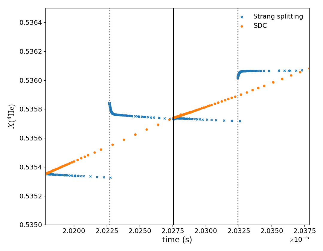
Figure 3: Helium mass fraction as a function of time over two timesteps for a detonation test problem with a 19-isotope reaction network. The points represent individual calls to the righthand side function of our reaction network (see Eq. 1) and the density of points indicates how hard the integrator is working. For the Strang case, we see that the first half of the reactions brings us off of the smooth solution (represented by the SDC curve), then the advection overcorrects, resulting in a discontinuous jump, and finally the second half of the reactions works to bring the state back to the solution curve.

Other ways to make the simulation less expensive can include a subgrid model. Flame models are commonly used for Type Ia supernovae. There however, the flame is thin compared to the scale height, so a simple model can represent the unresolved flame on the grid. For the XRB, the flame thickness is a non-trivial fraction of the pressure scale height and further, the laminar flame properties will change strongly over the height of the burning layer (see [9]). This makes traditional flame models a poor fit. Methods that use even something as simple as subzone burning (e.g. [34]) may help capture the energetics with lower resolution. This can be implemented using the AMR machinery. This may help a little, but will still be insufficient for full star models.

If we continue to resolve the flame structure, then we need to be smarter (and more aggressive) about our grid refinement strategy. Currently, we put the entire fuel layer on the finest grid, but for the material ahead of the flame, we could keep it at lower resolution until the flame reaches it. The main obstacle is that we need to keep the fuel ahead of the flame in hydrostatic equilibrium, and keeping it refined accomplishes this well. Using well-balanced schemes [35] can help us retain hydrostatic equilibrium (HSE) in the lower refined regions, reducing the number of zones needed to maintain fidelity, but we would still need a way to regrid the layer ahead of the flame to higher resolution to accurately capture the burning dynamics. To accomplish this, we envision building a refinement strategy that does interpolation of the data onto the newly refined grids enforcing hydrostatic equilibrium. This can allow us to keep only a narrow fully refined region that “slides” along the surface of the neutron star keeping pace with the advancing flame. When using mesh refinement the overall costs are dominated by the number of zones at the finest resolution, so such a scheme would greatly reduce the computational costs. This is a longer term development.

All of the above developments still involve fully compressible hydrodynamics, but multiscale methods [36] where we couple different hydrodynamics solvers together in a single simulation may ultimately be needed to model the full star while resolving the burning front. Such techniques rely on it being possible to decompose the dynamics of the system into two scales, e.g. a short and a long lengthscale, and that the processes at each scale are at most weakly coupled with each other. In the context of XRBs, one possibility for multiscale modeling would be to model the large scale dynamics using a shallow water model (like that of [8]) to capture the effects of the Coriolis force, and use a low Mach number or a fully compressible model in the vicinity of the burning front to capture the turbulent burning processes. Given that the computational costs of the shallow water model would be negligible compared to those of the low Mach/compressible model, the overall cost of this multiscale model would be determined by the size of the low Mach/compressible region only. This approach would therefore allow us to capture dynamics across the full star without sacrificing resolution around the flame. As with the more aggressive gridding strategy above, the hybrid approach reduces the number of zones with the largest computational cost through mesh refinement, and also reduces the computational costs where possible by employing cheaper physical models in regions where this is possible. An example of coupling compressible and low Mach number models implemented using the AMReX framework, but in a terrestrial context, is [37]. An initial implementation, [38], in an astrophysical context, coupling shallow water to compressible models in both Newtonian and relativistic gravity, indicates that considerable computational efficiencies are possible, but that close attention to the coupling between the models is needed.

4 Summary

XRBs are multiscale, multiphysics problems that are challenging to model. Nevertheless, significant progress has been made in multidimensional models of these events, through a set of complementary algorithmic approaches. Future advances in computer architectures and algorithms will allow for even more realistic models of these events, and help us connect to observations, ultimately telling us about the neutron star itself.

The work at Stony Brook was supported by DOE/Office of Nuclear Physics grant DE-FG02-87ER40317 and contract 7418390 with Lawrence Berkeley National Laboratory as part of the Exascale Compute Project ExaStar collaboration. The work at LBNL was supported by the DOE Office of Advanced Scientific Computing Research under Contract No, DE-AC02-05CH11231. YC is supported by the European Union Horizon 2020 research and innovation programme under the Marie Sklodowska-Curie Global Fellowship grant agreement No 703916. An award of computer time was provided by the Innovative and Novel Computational Impact on Theory and Experiment (INCITE) program. This research used resources of the Oak Ridge Leadership Computing Facility at the Oak Ridge National Laboratory, which is supported by the Office of Science of the U.S. Department of Energy under Contract No. DE-AC05-00OR22725. This research used resources of the National Energy Research Scientific Computing Center, which is supported by the Office of Science of the U.S. Department of Energy under Contract No. DE-AC02-05CH11231. Visualizations were done using yt [39]. This research has made use of NASA’s Astrophysics Data System Bibliographic Services.

References

- [1] Suleimanov V, Poutanen J and Werner K 2011 A&A 527 A139 (Preprint 1009.6147)
- [2] Kajava J J E, Nättilä J, Poutanen J, Cumming A, Suleimanov V and Kuulkers E 2017 MNRAS 464 L6–L10 (Preprint 1608.06801)
- [3] Steiner A W, Lattimer J M and Brown E F 2010 Astrophysical Journal 722 33–54 (Preprint 1005.0811)
- [4] Özel F, Baym G and Güver T 2010 Phys. Rev. D 82 101301 (Preprint 1002.3153)
- [5] Bhattacharyya S and Strohmayer T E 2006 636 L121–L124 (Preprint arXiv:astro-ph/0509369)
- [6] Bhattacharyya S and Strohmayer T E 2007 666 L85–L88
- [7] Galloway D K and Keek L 2017 ArXiv e-prints (Preprint 1712.06227)
- [8] Spitkovsky A, Levin Y and Ushomirsky G 2002 Astrophysical Journal 566 1018–1038
- [9] Timmes F X 2000 ApJ 528 913–945 source code obtained from http://cococubed.asu.edu/code_pages/kap.shtml
- [10] Woosley S E, Heger A, Cumming A, Hoffman R D, Pruet J, Rauscher T, Fisker J L, Schatz H, Brown B A and Wiescher M 2004 Astrophysical Journal Supplement 151 75–102
- [11] Fisker J L, Schatz H and Thielemann F K 2008 ApJS 174 261–276
- [12] Schatz H, Bildsten L, Cumming A and Wiescher M 1999 Astrophysical Journal 524 1014–1029 (Preprint arXiv:astro-ph/9905274)
- [13] Schatz H, Aprahamian A, Barnard V, Bildsten L, Cumming A, Ouellette M, Rauscher T, Thielemann F and Wiescher M 2001 Physical Review Letters 86 3471–3474 (Preprint arXiv:astro-ph/0102418)
- [14] Schatz H 2006 International Symposium on Nuclear Astrophysics - Nuclei in the Cosmos p 2.1
- [15] Lin D J, Bayliss A and Taam R E 2006 ApJ 653 545–557
- [16] Malone C M, Nonaka A, Almgren A S, Bell J B and Zingale M 2011 Astrophysical Journal 728 118 (Preprint 1012.0609)
- [17] Malone C M, Zingale M, Nonaka A, Almgren A S and Bell J B 2014 Astrophysical Journal 788 115
- [18] Zingale M, Malone C M, Nonaka A, Almgren A S and Bell J B 2015 Astrophysical Journal 807 60 (Preprint 1410.5796)
- [19] Almgren A S, Bell J B, Rendleman C A and Zingale M 2006 Astrophysical Journal 637 922–936 paper I
- [20] Zingale M, Timmes F X, Fryxell B, Lamb D Q, Olson K, Calder A C, Dursi L J, Ricker P, Rosner R, MacNeice P and Tufo H M 2001 Astrophysical Journal Supplement 133 195–220
- [21] Harpole A and Hawke I 2018 ArXiv e-prints (Preprint 1806.07301)
- [22] Cavecchi Y, Watts A L, Braithwaite J and Levin Y 2013 Monthly Notices of the Royal Astronomical Society 434 3526–3541 (Preprint 1212.2872)
- [23] Cavecchi Y, Watts A L, Levin Y and Braithwaite J 2015 MNRAS 448 445–455 (Preprint 1411.2284)
- [24] Cavecchi Y, Levin Y, Watts A L and Braithwaite J 2016 MNRAS 459 1259–1275 (Preprint 1509.02497)
- [25] Wilson-Hodge C A, Ray P S, Gendreau K, Chakrabarty D, Feroci M, Maccarone T, Arzoumanian Z, Remillard R A, Wood K, Griffith C and STROBE-X Collaboration 2017 American Astronomical Society Meeting Abstracts (American Astronomical Society Meeting Abstracts vol 229) p 309.04
- [26] Zhang S N et al. 2016 Space Telescopes and Instrumentation 2016: Ultraviolet to Gamma Ray (Proc. SPIE vol 9905) p 99051Q (Preprint 1607.08823)
- [27] in ’t Zand J J M et al. 2018 Science China Physics, Mechanics & Astronomy 62 29506 ISSN 1869-1927 URL https://doi.org/10.1007/s11433-017-9186-1
- [28] Almgren A S, Beckner V E, Bell J B, Day M S, Howell L H, Joggerst C C, Lijewski M J, Nonaka A, Singer M and Zingale M 2010 Astrophysical Journal 715 1221–1238 (Preprint 1005.0114)
- [29] Zingale M, Almgren A S, Barrios Sazo M G, Beckner V E, Bell J B, Friesen B, Jacobs A M, Katz M P, Malone C M, Nonaka A J, Willcox D E and Zhang W 2017 ArXiv e-prints Accepted to Proceedings of AstroNum 2017 (Preprint 1711.06203)
- [30] Katz M P, Zingale M, Calder A C, Swesty F D, Almgren A S and Zhang W 2016 Astrophysical Journal 819 94 (Preprint 1512.06099)
- [31] Strang G 1968 SIAM J. Numerical Analysis 5 506–517
- [32] Nonaka A, Bell J B, Day M S, Gilet C, Almgren A S and Minion M L 2012 Combustion Theory and Modelling 16 1053–1088 (Preprint https://doi.org/10.1080/13647830.2012.701019) URL https://doi.org/10.1080/13647830.2012.701019
- [33] Brown P N, Byrne G D and Hindmarsh A C 1989 SIAM J. Sci. Stat. Comput. 10 1038–1051
- [34] Wang W, Shu C W, Yee H and Sj??green B 2012 Journal of Computational Physics 231 190 – 214 ISSN 0021-9991 URL http://www.sciencedirect.com/science/article/pii/S0021999111005250
- [35] Käppeli R and Mishra S 2016 A&A 587 A94
- [36] Weinan E 2011 Principles of multiscale modeling (Cambridge University Press)
- [37] Motheau E, Duarte M, Almgren A and Bell J B 2018 Journal of Computational Physics 372 1027–1047 ISSN 00219991 URL https://linkinghub.elsevier.com/retrieve/pii/S0021999118300469
- [38] Harpole A 2018 Multiscale modelling of neutron star oceans Ph.D. thesis University of Southampton URL https://eprints.soton.ac.uk/id/eprint/422175
- [39] Turk M J, Smith B D, Oishi J S, Skory S, Skillman S W, Abel T and Norman M L 2011 Astrophysical Journal Supplement 192 9 (Preprint 1011.3514)