CASTRO: A New Compressible Astrophysical Solver. I. Hydrodynamics and Self-Gravity
Abstract
We present a new code, CASTRO, that solves the multicomponent compressible hydrodynamic equations for astrophysical flows including self-gravity, nuclear reactions and radiation. CASTRO uses an Eulerian grid and incorporates adaptive mesh refinement (AMR). Our approach to AMR uses a nested hierarchy of logically-rectangular grids with simultaneous refinement in both space and time. The radiation component of CASTRO will be described in detail in the next paper, Part II, of this series.
1 Introduction
In this paper, Part I of a two-part series, we present a new code, CASTRO, that solves the multicomponent compressible hydrodynamic equations with a general equation of state for astrophysical flows. Additional physics include self-gravity, nuclear reactions, and radiation. CASTRO uses an Eulerian grid and incorporates adaptive mesh refinement (AMR). Our approach to AMR uses a nested hierarchy of logically-rectangular grids with simultaneous refinement of the grids in both space and time. Spherical (in 1D), cylindrical (in 1D or 2D), and Cartesian (in 1D, 2D or 3D) coordinate systems are supported. The radiation component of CASTRO will be described in detail in the next paper, Part II, of this series.
There are a number of other adaptive mesh codes for compressible astrophysical flows, most notably, ENZO (O’Shea et al., 2005), FLASH (Fryxell et al., 2000), and RAGE (Gittings et al., 2008). CASTRO differs from these codes in several ways. CASTRO uses an unsplit version of the piecewise parabolic method, PPM, with new limiters that avoid reducing the accuracy of the scheme at smooth extrema; the other codes are based on operator-split hydrodynamics, though the most recent release of FLASH, version 3.2, includes an unsplit MUSCL-Hancock scheme. The different methodologies also vary in their approach to adaptive mesh refinement. RAGE uses a cell-by-cell refinement strategy while the other codes use patch-based refinement. FLASH uses equal size patches whereas ENZO and CASTRO allow arbitrary sized patches. ENZO and FLASH enforce a strict parent-child relationship between patches; i.e., each refined patch is fully contained within a single parent patch; CASTRO requires only that the union of fine patches be contained within the union of coarser patches with a suitable proper nesting. Additionally, FLASH and RAGE use a single time step across all levels while CASTRO and ENZO support subcycling in time. All four codes include support for calculation of self-gravity.
It is worth noting that CASTRO uses the same grid structure as the low Mach number astrophysics code, MAESTRO (see, e.g., Nonaka et al. (2010)). This will enable us to map the results from a low Mach number simulation, such as that of the convective period and ignition of a Type Ia supernova, to the initial conditions for a compressible simulation such as that of the explosion itself, thus taking advantage of the accuracy and efficiency of each approach as appropriate.
2 Hydrodynamics
In CASTRO we evolve the fully compressible equations forward in time. The equations expressing conservation of mass, momentum, and total energy are:
| (1) | |||||
| (2) | |||||
| (3) |
Here , , and are the mass density, velocity vector, and total energy per unit mass, respectively. The total energy, , where is the specific internal energy. The pressure, is defined by a user-supplied equation of state, and is the gravitational acceleration vector. The source terms, , , and are user-specified external source terms for the mass, momentum, and energy equations, respectively. For reacting flows, we evolve equations for mass fractions, :
| (4) |
where the production rates, , for species are defined by a user-supplied reaction network. The reaction network also determines the energy generation rate . The mass fractions are subject to the constraint that . Again, a user-specified external source, , may be specified. Finally, CASTRO includes passively advected quantities, , and auxiliary variables, that satisfy
| (5) | |||||
| (6) |
Advected and auxiliary variables are updated similarly, but they differ in their usage. In particular, auxiliary variables are passed into the equation of state routines. Examples of auxiliary and advected variables, respectively, might include the electron fraction, , used in simulations of core collapse supernovae, and angular momentum in two-dimensional simulations of a rotating star in cylindrical (axisymmetric) coordinates. Both of these evolution equations include user-specified sources, and . We refer to as the conserved variables.
3 Equation of State and Reaction Network
CASTRO is written in a modular fashion so that the routines for the equation of state and reaction network can be supplied by the user. However, for the test problems presented later we use routines that come with the CASTRO distribution.
Each equation of state must provide an interface for obtaining thermodynamic quantities from , and . One equation of state which is supplied with the CASTRO distribution is the gamma-law equation of state, which relates pressure and temperature, , to and via:
| (7) |
Here, is the ratio of specific heats (e.g. for a monatomic gas), is Boltzmann’s constant, is the mass of the proton, and the mean molecular weight, , is determined by
| (8) |
with the atomic weight of species .
The CASTRO distribution also includes more complex equations of state describing stellar matter, including the Helmholtz equation of state (Timmes & Swesty, 2000; Fryxell et al., 2000) which includes degenerate/relativistic electrons, ions (as a perfect gas), and radiation, and the Lattimer-Swesty equation of state, which describes dense nuclear matter (Lattimer & Swesty, 1991). For tabular equations of state, it is common that , , and are inputs, in which case a Newton-Raphson iteration is typically used to invert the equation of state.
CASTRO can support any general reaction network that takes as inputs the density, temperature, and mass fractions, and returns updated mass fractions and the energy release (or decrease). The input temperature is computed from the equation of state before each call to the reaction network. In general, we expect the reaction network to evolve the species according to:
| (9) |
Reaction rates can be extremely temperature-sensitive, so in most cases, the reaction network should be written to evolve the temperature for the purposes of evaluating the rates. Close to nuclear statistical equilibrium, the energy release and change in abundances can rapidly change sign if the rates are not evaluated with a temperature field consistent with the evolving energy (Müller, 1986). At the end of the burning step, we use the energy release to update the total energy, . The density remains unchanged during the burning.
4 Gravity
CASTRO supports several different options for how to specify and/or compute the gravitational acceleration. The simplest option is a gravitational field that is constant in space and time; this can be used for small-scale problems in which the variation of gravity throughout the computational domain is negligible. This option is available in 1D Cartesian coordinates, 2D cylindrical or Cartesian coordinates, and 3D Cartesian coordinates.
A second approach uses a monopole approximation to compute a radial gravity field consistent with the mass distribution. Because the algorithm subcycles in time we construct a separate 1D radial density profile at each level at each time needed. Once the radial density profile is defined, gravity is computed as a direct integral of the mass enclosed. This field is then interpolated back onto the original grids.
The most general option is to solve the Poisson equation for self-gravity, i.e. solve
| (10) |
for , and define This can be used in any of the coordinate systems. At boundaries away from the star we set inhomogeneous Dirichlet boundary conditions for ; these values are determined by computing the monopole approximation for on the coarsest level, integrating this profile radially outward to create and interpolating onto the domain boundaries to define the boundary conditions for the solve. Boundaries that pass through the center of the star use symmetry boundary conditions.
The Poisson equation is discretized using standard finite difference approximations and the resulting linear system is solved using geometric multigrid techniques, specifically V-cycles and red-black Gauss-Seidel relaxation. For multilevel calculations, special attention is paid to the synchronization of the gravitational forcing across levels, which will be discussed in Section 6.
There is also an option to add the gravitational forcing due to a specified point mass to either of the self-gravity options described above.
5 Single-Level Integration Algorithm
The time evolution of can be written in the form
| (11) |
where is the flux vector, are the reaction source terms, and are the non-reaction source terms, which includes any user-defined external sources, . We use Strang splitting (Strang, 1968) to discretize the advection-reaction equations. In other words, to advance the solution, by one time step, we first advance the nuclear reaction network by ,
| (12a) | |||
| then advect the solution by , ignoring the reaction terms, | |||
| (12b) | |||
| and finally advance the nuclear reaction network by another , | |||
| (12c) | |||
The construction of is purely explicit, and based on an unsplit Godunov method. The solution, and source terms, are defined on cell centers; we predict the primitive variables, , from cell centers at time to edges at time and use an approximate Riemann solver to construct fluxes, on cell faces. This algorithm is formally second-order in both space and time.
5.1 Single-Level Flow Chart
At the beginning of each time step, we assume that, in the case of self-gravity, is defined consistently with the current mass distribution in The algorithm at a single level of refinement is composed of the following steps:
- Step 1:
-
Advance the nuclear reaction network through a time interval of .
Define with the exception of
(13) (14) where and are computed using calls to the user-defined reaction network. Note that is unchanged during this step.
- Step 2:
-
Advect the solution through .
Advance the solution using time-centered fluxes and an explicit representation of the source term, neglecting the contribution from reactions which are taken into account in Steps 1 and 4 (the asterisk superscript notation indicates that we will later correct this state to effectively time-center the source terms):
(15) where
(16) The construction of the fluxes is described in detail in Section 5.2. We note that in the single-level algorithm we can use the gravitational forcing computed in Step 3 of the previous time step, since the density has not changed.
After the advective update, we ensure that the solution is physically meaningful by forcing the density to exceed a non-negative, user-defined minimum value. We also ensure that the mass fractions are all non-negative and sum to one.
We also have an option for a user-defined sponge in order to prevent the velocities in the upper atmosphere from becoming too large, and subsequently, the time step from becoming too small. We multiply the velocity by where is the sponge strength, and is a smooth function of density that varies from 0 to 1. Full details of the sponge are given in Zingale et al. (2009). Finally, we adjust to be consistent with .
- Step 3:
-
Correct the solution with time-centered source terms and compute gravity at .
We correct the solution by effectively time-centering the source terms. First, we correct with updated external sources:
(17) Next, we evaluate gravity using If using full gravity we solve
(18) where we supply an initial guess for from the previous solve. In the single-level algorithm described here, is saved to be used as in Step 2 of the next time step. This suffices in the single-level algorithm because does not change between the end of Step 3 of one time step and the start of Step 2 of the next time step.
We then correct the solution with the updated gravity:
(19) (20) For all other conserved variables other than and . We note here that the time discretization of the gravitational forcing terms differs from that in the FLASH (Fryxell et al., 2000) and ENZO (O’Shea et al., 2005) codes, where the gravitational forcing at is computed by extrapolation from values at and (see also Bryan et al. 1995). Our discretization of the gravitational terms is consistent with our predictor-corrector approach in the handling of other source terms.
- Step 4:
-
Advance the nuclear reaction network through a time interval of .
Define with the exception of
(21) (22) We also include an option to modify any component of the new-time state as needed to account for special user requirements.
- Step 5:
-
Compute the new time step.
The time step is computed using the standard CFL condition for explicit methods, with additional constraints (such as one based on rate of burning) possible as needed. The user sets a CFL factor, between 0 and 1. The sound speed, , is computed by the equation of state, and for a calculation in dimensions,
(23) where
(24) is the minimum taken over all computational grid cells in the domain.
This concludes the single-level algorithm description. We note that whenever the kinetic energy dominates the total energy, making the calculation of from numerically unreliable, we use a method similar to the dual-energy approach described in Bryan et al. (1995) to compute the internal energy with sufficient precision. In practice, this involves evolving in time and using this solution when appropriate.
5.2 Construction of Fluxes
We use an unsplit Godunov method with characteristic tracing and full corner coupling in 3D (Miller & Colella, 2002) to compute time-centered edge states. We have replaced the PPM limiters in Miller & Colella (2002) with an updated PPM algorithm that is designed to preserve accuracy at smooth extrema and is insensitive to asymmetries caused by roundoff error (Colella & Sekora, 2008; McCorquodale & Colella, 2010). CASTRO also has options to use the unsplit piecewise-linear algorithm described in Colella (1990); Saltzman (1994), or to retain the PPM limiters in Miller & Colella (2002), which were originally developed in Colella & Woodward (1984) using a split integrator.
There are four major steps in the construction of the face-centered fluxes, that are used in Step 2 in Section 5.1 to update the solution. We also include details on the solution of the Riemann problem. In summary,
Step 2.1: Rewrite the state, , in terms of primitive variables, .
Step 2.2: Construct a piecewise parabolic approximation of within each cell.
Step 2.3: Predict average values of on edges over the time step using characteristic extrapolation.
Step 2.4: Compute fluxes, using an approximate Riemann problem solver.
We expand each of these steps in more detail below.
- Step 2.1:
-
Compute primitive variables and source terms.
We define . The pressure, , is computed through a call to the equation of state using , and . Note that we also include in ; this quantity is used in the approximate Riemann solver to avoid an EOS call to evaluate the energy flux, analogous to the effective dynamics for in the Colella & Glaz (1985) approximate Riemann solver.
For the overall integration algorithm, we want to include the effect of source terms except for reactions in the characteristic tracing (Step 2.2). (Reactions are treated separately using a symmetric operator split approach in Steps 1 and 4 of the algorithm.) The time evolution equations written in terms of the primitive variables, and omitting contributions from reactions, are
where
(25) Here, is the sound speed, defined as , with , with the entropy. The remaining thermodynamic derivatives are , , and . Often, the equation of state is a function of , , and , and returns derivatives with these quantities held constant. In terms of the latter derivatives, our required thermodynamic derivatives are:
- Step 2.2:
-
Reconstruct parabolic profiles within each cell.
In this step we construct a limited piecewise parabolic profile of each in (we use to denote an arbitrary primitive variable from from ). These constructions are performed in each coordinate direction separately. The default option in CASTRO is to use a new limiting procedure that avoids reducing the order of the reconstruction at smooth local extrema. The details of this construction are given in Colella & Sekora (2008); McCorquodale & Colella (2010). In summary:
-
•
Step 2.2a: For each cell, we compute the spatial interpolation of to the high and low faces of cell using a limited cubic interpolation formula. These interpolants are denoted by and .
-
•
Step 2.2b: Construct quadratic profiles using , and .
(27) (28) (29) where is the mesh spacing in the direction of interpolation. Also, as in Miller & Colella (2002), we compute a flattening coefficient, , used in the edge state prediction to further limit slopes near strong shocks. The computation of is identical to the approach used in FLASH (Fryxell et al., 2000), except that a flattening coefficient of 1 indicates that no additional limiting takes place, whereas a flattening coefficient of 0 means we effectively drop order to a first-order Godunov scheme, which is opposite of the convention used in FLASH.
-
•
- Step 2.3:
-
Characteristic extrapolation.
We begin by extrapolating to edges at The edge states are dual-valued, i.e., at each face, there is a left state and a right state estimate, denoted and (we write the equations in 1D for simplicity). The spatial extrapolation is one-dimensional, i.e., transverse derivatives are omitted and accounted for later.
-
•
Step 2.3a: Integrate the quadratic profiles. We are essentially computing the average value swept out by the quadratic profile across the face assuming the profile is moving at a speed , where is a standard wave speed associated with gas dynamics.
Define the following integrals, where :(30a) (30b) Substituting (27) gives:
(31a) (31b) -
•
Step 2.3b: Obtain a left and right edge state at by applying a characteristic tracing operator (with flattening) to the integrated quadratic profiles. Note that we also include the explicit source term contribution.
(32a) (32b) In non-Cartesian coordinates, volume source terms are added to the traced states. Here, and are the standard right column and left row eigenvectors associated with the equations of gas dynamics (see Toro 1997).
An unsplit approximation that includes full corner coupling is constructed by constructing increasingly accurate approximations to the transverse derivatives. The details follow exactly as given in Section 4.2.1 in Miller & Colella (2002), except for the solution of the Riemann problem, which is described in Step 2.4.
-
•
- Step 2.4:
-
Compute fluxes
The fluxes are computed using an approximate Riemann solver. The solver used here is essentially the same as that used in Colella et al. (1997), which is based on ideas discussed in Bell et al. (1989). This solver is computationally faster and considerably simpler than the approximate Riemann solver introduced by Colella & Glaz (1985). The Colella and Glaz solver was based on an effective dynamics for and was designed for real gases that are well-approximated by this type of model. The approximate Riemann solver used in CASTRO is suitable for a more general convex equation of state.
As with other approximate Riemann solvers, an important design principle is to avoid additional evaluations of the equation of state when constructing the numerical flux. For that reason, we include in and compute . The information carried in is overspecified but it allows us to compute an energy flux without an inverse call to the equation of state.
The numerical flux computation is based on approximating the solution to the Riemann problem and evaluating the flux along the ray. The procedure is basically a two-step process in which we first approximate the solution in phase space and then interpret the phase space solution in real space.
-
•
Step 2.4a: To compute the phase space solution we first solve for and , the pressure between the two acoustic waves and the velocity of the contact discontinuity, respectively. These quantities are computed using a linearized approximation to the Rankine-Hugoniot relations. We first define by using the cell-centered values on either side of the interface. Next, we compute Lagrangian sound speeds, and and the corresponding Eulerian sound speeds . Then,
(33a) (33b) From and we can compute
(34a) (34b) (34c) (34d) where generically represents advected quantities (which includes transverse velocity components). Here, the notation refers to values on the left and right side of the contact discontinuity.
-
•
Step 2.4b: The next step in the approximate Riemann solver is to interpret this phase space solution. If then the contact discontinuity is moving to the right and numerical flux depends on the speed and structure of the acoustic wave connecting and associated with the eigenvalue. Similarly if then the contact is moving to the left and the numerical flux depends on the speed and structure of the acoustic wave connecting and associated with the eigenvalue. Here we discuss in detail the case in which the other case is treated analogously.
For we define and . If then the wave is a shock wave and we define a shock speed . For that case if then the shock is moving to the right and we define the Godunov state ; otherwise . The rarefaction case is somewhat more complex. If both and are negative, then the rarefaction fan is moving to the left and . Similarly, if both and are positive, then the rarefaction fan is moving to the right and . However, in the case in which , the rarefaction spans the ray and we need to interpolate the solution. For this case, we define
(35) where . This choice of corresponds to linearly interpolating through the rarefaction to approximate the state that propagates with zero speed.
As noted above the case in which is treated analogously. When we compute by averaging and . For the Riemann problem approximation, we allow for user-specified floors for , and to prevent the creation of non-physical values.
The fluxes can then be evaluated from the final . A small quadratic artificial viscosity that is proportional to the divergence of the velocity field is added to the flux in order to add additional dissipation at strong compressions. We also scale all the species fluxes so that they sum to the density flux, as in the sCMA algorithm described by Plewa & Müller (1999).
-
•
6 AMR
Our approach to adaptive mesh refinement in CASTRO uses a nested hierarchy of logically-rectangular grids with simultaneous refinement of the grids in both space and time. The integration algorithm on the grid hierarchy is a recursive procedure in which coarse grids are advanced in time, fine grids are advanced multiple steps to reach the same time as the coarse grids and the data at different levels are then synchronized.
The AMR methodology was introduced by Berger & Oliger (1984); it has been demonstrated to be highly successful for gas dynamics by Berger & Colella (1989) in two dimensions and by Bell et al. (1994) in three dimensions.
6.1 Creating and Managing the Grid Hierarchy
6.1.1 Overview
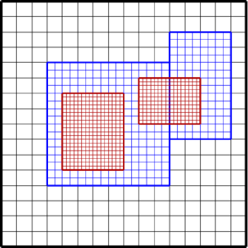
The grid hierarchy is composed of different levels of refinement ranging from coarsest () to finest (). The maximum number of levels of refinement allowed, , is specified at the start of a calculation. At any given time in the calculation there may not be that many levels in the hierarchy, i.e. can change dynamically as the calculation proceeds as long as Each level is represented by the union of non-overlapping rectangular grids of a given resolution. Each grid is composed of an even number of cells in each coordinate direction; cells are the same size in each coordinate direction but grids may have different numbers of cells in each direction. Figure 1 shows a cartoon of AMR grids in two dimensions with two levels of refinement.
In this implementation, the refinement ratio between levels and which we call is always two or four, with the same factor of refinement in each coordinate direction. The grids are properly nested, in the sense that the union of grids at level is contained in the union of grids at level . Furthermore, the containment is strict in the sense that, except at physical boundaries, the level grids are large enough to guarantee that there is a border at least level cells wide surrounding each level grid (grids at all levels are allowed to extend to the physical boundaries so the proper nesting is not strict there). The parameter is two for factor two refinement, and one for factor four refinement, since four ghost cells are needed for the PPM algorithm.
6.1.2 Error Estimation and Regridding
We initialize the grid hierarchy and regrid following the procedure outlined in Bell et al. (1994). Given grids at level we use an error estimation procedure to tag cells where the error, as defined by user-specified routines, is above a given tolerance. Typical error criteria include first or second derivatives of the state variables or quantities derived from the state variables, or the state variables or derived quantities themselves. A user can specify that any or all of the criteria must be met to refine the cell; one can also specify criteria that ensure that a cell not be refined. For example, one could specify that a cell be refined if and ( or ), where and are constants specified by the user.
The tagged cells are grouped into rectangular grids at level using the clustering algorithm given in Berger & Rigoutsos (1991). These rectangular patches are refined to form the grids at level . Large patches are broken into smaller patches for distribution to multiple processors based on a user-specified max_grid_size parameter.
At the beginning of every level time steps, where is specified by the user at run-time, new grid patches are defined at all levels and higher if In regions previously covered by fine grids the data is simply copied from old grids to new; in regions which are newly refined, data is interpolated from underlying coarser grids.
6.1.3 Enlarging the Domain
The finest resolution of a calculation can vary in time; however, the coarsest resolution covering the domain does not change during a single run. However, a feature has been added to the CASTRO distribution that allows a user to restart a calculation in a larger domain covered by a coarser resolution, provided the data exists to initialize the larger domain. This is useful in simulations during which a star expands dramatically, for example. Using this strategy one could periodically stop the simulation, double the domain size, and restart the calculation in the larger domain.
6.2 Multilevel Algorithm
6.2.1 Overview
The multilevel time stepping algorithm can most easily be thought of as a recursive procedure. In the case of zero or constant gravity, to advance level the following steps are taken. Here the phrase, “Advance ” refers to Steps 1–4 of the single-level algorithm described in the previous section.
-
•
If compute the new time steps for all levels as follows
-
–
compute the appropriate time step for each level, using the procedure described in Step 5 of the previous section,
-
–
define as the ratio of the level 0 cell size to the level cell size
-
–
define
-
–
define for all ,
-
–
-
•
Advance at level in time as if it is the only level, filling boundary conditions for from level if level , and from the physical domain boundaries.
-
•
If
-
–
Advance at level () for time steps with time step
-
–
Synchronize the data between levels and
-
*
Volume average at level onto level grids.
-
*
Correct in all level cells adjacent to but not covered by the union of level grids through an explicit refluxing operation as described in Berger & Colella (1989).
-
*
-
–
6.2.2 Monopole Gravity
When we use the monopole gravity assumption in a multilevel simulation, we can no longer exploit the fact that at level at the end of Step 3 of one time step is unchanged when one reaches the beginning of Step 2 of the next level time step. If then potential changes in come from two sources:
-
•
at level under the level grids is replaced by the volume average of at level ;
-
•
the explicit refluxing step between levels and modifies on all level cells adjacent to but not covered by the union of level grids.
In addition, because the grids are dynamically created and destroyed through regridding, at the beginning of Step 2 of a level time step, there may not be a value for from the previous step, because this region of space was previously not covered by level grids.
In order to address all of these changes, we simply compute at the beginning of Step 2 of each time step at each level, rather than copying it from from Step 3 of the previous time step as in the single-level algorithm. This captures any changes in grid structure due to regridding, and reflects any changes in density due to refluxing or volume averaging.
6.2.3 Full Gravity Solve
Overview
Solving the Poisson equation for self-gravity on a multilevel grid hierarchy introduces additional complications. We start by defining some necessary notation. We define as an approximation to at level with the assumption that Dirichlet boundary conditions are supplied on the boundary of the union of level grids (we allow more general boundary conditions at physical boundaries), and define a level solve as the process of solving
at level
We define as the composite grid approximation to on levels through , and define a composite solve as the process of solving
on levels through The solution to the composite solve satisfies
at level , but satisfies
for only on the regions of each level not covered by finer grids or adjacent to the boundary of the finer grid region. In regions of a level grid covered by level grids the solution is defined as the volume average of the solution at ; in level cells immediately adjacent to the boundary of the union of level grids, a modified interface operator is used that reflects the geometry of the interface (see, e.g., Almgren et al. (1998) for details of the multilevel cell-centered interface stencil).
In an algorithm without subcycling one can perform a composite solve at every time step, as described in Ricker (2008), to solve for on all levels. Because the CASTRO algorithm uses subcycling in time, however, we must use level solves at times when the solution is not defined at all levels, and then synchronize the solutions at different levels as appropriate. Even without changes in due to volume averaging and refluxing, replacing a composite solve by separate level solves generates a mismatch in the normal gradient of at the boundary between each level. We correct these mismatches with a multilevel correction solve, which is a two-level composite solve for a correction to In addition to correcting the solutions once the mismatch is detected, we add a correction term to later level solve solutions in order to minimize the magnitude of the correction that will be needed.
Multilevel Algorithm
At the start of a calculation, we perform a composite solve from level 0 through to compute at all levels. In addition, after every regridding step that creates new grids at level and higher, a composite solve from level through is used to compute at those levels.
Following an approach similar to that described in Miniati & Colella (2007), at the start and end of each level time step we perform a level solve to compute The difference between and at the start of the time step is stored in This difference is added to at the beginning and end of this level time step. Thus is identical to at the start of the time step; at the end of the time step it is an approximation to what the solution to the composite solve would be. In the event that the density does not change over the course of the time step, the effect of this lagged correction is to make at the end of the time step identical to at that time, thus there is no mismatch between levels to correct. In general, when the density is not constant, the effect of the lagged correction is to make the correction solve that follows the end of the time step much quicker. We now describe the two-level correction step. In the discussion below, we will refer to the two levels involved in a correction solve as the “coarse” and “fine” levels.
At the end of level time steps, when the level solution has reached the same point in time as the level solution, and after the volume averaging and refluxing steps above have been performed, we define two quantities on the coarse grid. The first is the cell-centered quantity, which carries the change in density at the coarse level due only to refluxing. The second is the face-centered flux register,
| (36) |
which accounts for the mismatch in the normal gradient of at coarse-fine interfaces. Here and represent area weighting factors on the coarse and fine levels, respectively. We define the composite residual, to be zero in all fine cells and in all coarse cells away from the union of fine grids, and
| (37) |
on all cells adjacent to the union of fine grids, where refers to the discrete divergence at the coarse level, where the only non-zero contribution comes from on the coarse-fine interface. We then solve
| (38) |
and define the update to gravity at both levels,
| (39) |
This update is used to correct the gravitational source terms. We define the new-time state after volume averaging but before refluxing as and the contributions to the solution on the coarse grid from refluxing as Then we can define the sync sources for momentum on the coarse and fine levels, , and , respectively as follows:
These momentum sources lead to the following energy sources:
The state at the coarse and fine levels is then updated using:
| , | ||||
| , |
(The factor of follows from the time-centering of the sources.)
To complete the correction step,
-
•
we add directly to and and interpolate to any finer levels and add it to the current at those levels. We note that at this point at levels and is identical to the solution that would have been computed using a two-level composite solve with the current values of density. Thus the new, corrected, at each level plays the role of in the next time step.
-
•
if level , we transmit the effect of this change in to the coarser levels by updating the flux register between level and level In particular, we set
(40)
Performance Issues
The multilevel algorithm is not as computationally expensive as it might appear. Because multigrid is an iterative solver, the cost of each solve is proportional to the number of V-cycles, which is a function of the desired reduction in residual. We can reduce the number of V-cycles needed in two ways. First, we can supply a good initial guess for the solution; second, we can lower the desired reduction in residual.
In the case of level solves, we always use from a previous level solve, when available, as a guess in the current level solve. Thus, even in a single-level calculation, from the beginning of the time step is used as a guess in the level solve at the end of the time step. If no regridding occurs, then at the end of one time step can be used as a guess for the level solve at the start of the next time step. The extent to which changes in a time step dictates the extent to which a new computation of gravity is needed, but this also dictates the cost of the update.
Similarly, there is no point in solving for to greater accuracy than we solve for When we do the correction solve for , we require only that the residual be reduced to the magnitude of the final residual from the level solve, not that we reduce the correction residual by the same factor. Thus, if the right-hand-side for the correction solve is already small, the cost of the correction solve will be significantly less than that of the initial level solve.
7 Software Design and Parallel Performance
7.1 Overview
CASTRO is implemented within the BoxLib framework, a hybrid C++ /Fortran90 software system that provides support for the development of parallel structured-grid AMR applications. The basic parallelization strategy uses a hierarchical programming approach for multicore architectures based on both MPI and OpenMP. In the pure-MPI instantiation, at least one grid at each level is distributed to each core, and each core communicates with every other core using only MPI. In the hybrid approach, where on each socket there are cores which all access the same memory, we can instead have one larger grid per socket, with the work associated with that grid distributed among the cores using OpenMP.
In BoxLib, memory management, flow control, parallel communications and I/O are expressed in the C++ portions of the program. The numerically intensive portions of the computation, including the multigrid solvers, are handled in Fortran90. The fundamental parallel abstraction in both the C++ and the Fortran90 is the MultiFab, which holds the data on the union of grids at a level. A MultiFab is composed of FAB’s; each FAB is an array of data on a single grid. During each MultiFab operation the FAB’s composing that MultiFab are distributed among the cores. MultiFab’s at each level of refinement are distributed independently. The software supports two data distribution schemes, as well as a dynamic switching scheme that decides which approach to use based on the number of grids at a level and the number of processors. The first scheme is based on a heuristic knapsack algorithm as described in Crutchfield (1991) and in Rendleman et al. (2000). The second is based on the use of a Morton-ordering space-filling curve.
Each processor contains meta-data that is needed to fully specify the geometry and processor assignments of the MultiFab’s. At a minimum, this requires the storage of an array of boxes specifying the index space region for each AMR level of refinement. One of the advantages of computing with fewer, larger grids in the hybrid OpenMP–MPI approach is that the size of the meta-data is substantially reduced.
7.2 Parallel Output
Data for checkpoints and analysis are written in a self-describing format that consists of a directory for each time step written. Checkpoint directories contain all necessary data to restart the calculation from that time step. Plotfile directories contain data for postprocessing, visualization, and analytics, which can be read using amrvis, a customized visualization package developed at LBNL for visualizing data on AMR grids, or VisIt (VisIt User’s Manual, 2005). Within each checkpoint or plotfile directory is an ASCII header file and subdirectories for each AMR level. The header describes the AMR hierarchy, including number of levels, the grid boxes at each level, the problem size, refinement ratio between levels, step time, etc. Within each level directory are the MultiFab files for each AMR level. Checkpoint and plotfile directories are written at user-specified intervals.
For output, each processor writes its own data to the appropriate MultiFab files. The output streams are coordinated to only allow one processor to write to a file at one time and to try to maintain maximum performance by keeping the number of open data streams, which is set at run time, equal to the number of files being written. Data files typically contain data from multiple processors, so each processor writes data from its associated grid(s) to one file, then another processor can write data from its associated grid(s) to that file. A designated I/O Processor writes the header files and coordinates which processors are allowed to write to which files and when. The only communication between processors is for signaling when processors can start writing and for the exchange of header information. We also use the C++ setbuf function for good single file performance. While I/O performance even during a single run can be erratic, recent timings on the Franklin machine (XT4) at NERSC indicate that CASTRO’s I/O performance, when run with a single level composed of multiple uniformly-sized grids, matches some of the top results for the N5 IOR benchmark (roughly 13GB/s) (Franklin Performance Monitoring, 2010). For more realistic simulations with multiple grids at multiple levels, CASTRO is able to write data at approximately 5 GB/s sustained, over half of the average I/O benchmark reported speed.
7.3 Parallel Restart
Restarting a calculation can present some difficult issues for reading data efficiently. In the worst case, all processors would need data from all files. If multiple processors try to read from the same file at the same time, performance problems can result, with extreme cases causing file system thrashing. Since the number of files is generally not equal to the number of processors and each processor may need data from multiple files, input during restart is coordinated to efficiently read the data. Each data file is only opened by one processor at a time. The IOProcessor creates a database for mapping files to processors, coordinates the read queues, and interleaves reading its own data. Each processor reads all data it needs from the file it currently has open. The code tries to maintain the number of input streams to be equal to the number of files at all times.
Checkpoint and plotfiles are portable to machines with a different byte ordering and precision from the machine that wrote the files. Byte order and precision translations are done automatically, if required, when the data is read.
7.4 Parallel Performance
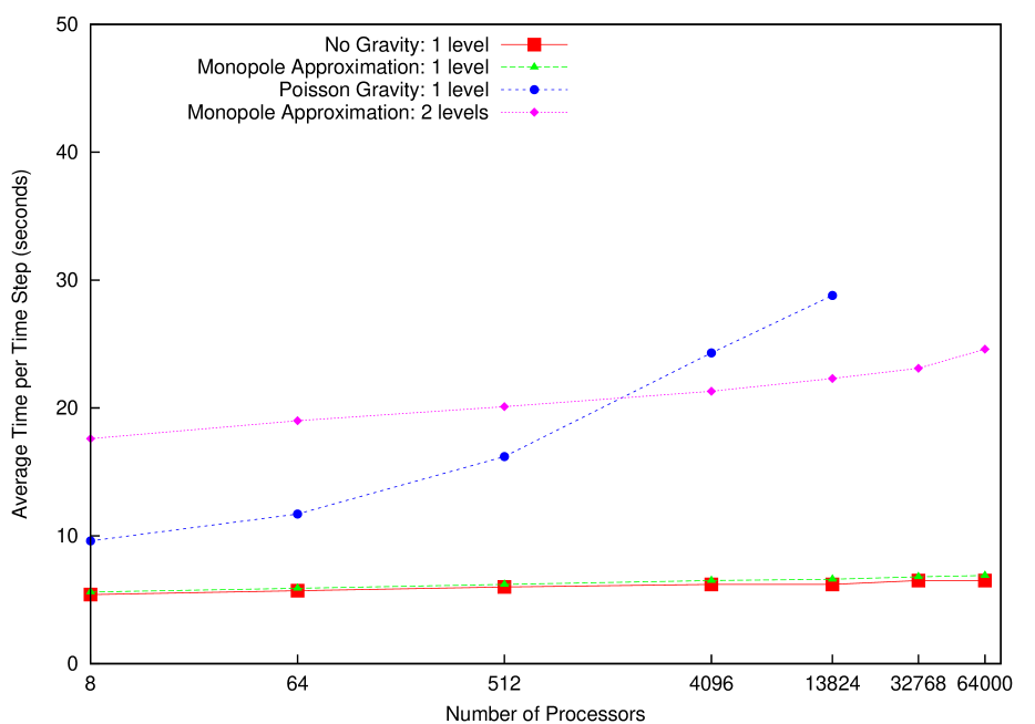
In Figure 2 we show the scaling behavior of the CASTRO code, using only MPI-based parallelism, on the jaguarpf machine at the Oak Ridge Leadership Computing Facility (OLCF). A weak scaling study was performed, so that for each run there was exactly one grid per processor. We ran the code with gravity turned off, with the monopole approximation to gravity, and with the Poisson solve for gravity. The monopole approximation to gravity adds very little to the run time of the code; with and without the monopole approximation the code scales excellently from 8 to 64,000 processors. For the 64,000 processor case without gravity, the time for a single core to advance one cell for one time step is 24.8 s.
Good scaling of linear solves is known to be much more difficult to achieve; we report relatively good scaling up to only 13,824 processors in the pure-MPI approach. An early strong scaling study contrasting the pure-MPI and the hybrid-MPI-OpenMP approaches for a domain shows that one can achieve at least a factor of 3 improvement in linear solver time by using the hybrid approach at large numbers of processors. Improving the performance of the linear solves on the new multicore architectures is an area of active research; more extensive development and testing is underway.
We also ran a scaling study with a single level of local refinement using the monopole gravity approximation. In this MPI-only study, there is one grid at each level for each processor. Because of subcycling in time, a coarse time step consists of a single step on the coarse grid and two steps on the fine grid. Thus, we would expect that the time to advance the multilevel solution by one coarse time step would be a factor of three greater than the time to advance the single-level coarse solution by one coarse time step, plus any additional overhead associated with AMR. From the data in the figure we conclude that AMR introduces a modest overhead, ranging from approximately 5% for the 8 processor case to 19% for the 64,000 processor case. By contrast, advancing a single-level calculation at the finer resolution by the same total time, i.e., two fine time steps, would require a factor of 16 more resources than advancing the coarse single-level solution.
8 Test Problems
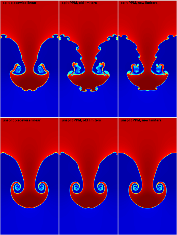
In this section we present a series of calculations demonstrating the behavior of the hydrodynamics, self-gravity, and reaction components of CASTRO. The first set contains three one-dimensional shock tube problems, including Sod’s problem, a double rarefaction problem, and a strong shock problem. We follow this with Sedov-Taylor blast waves computed in 1D spherical coordinates, 2D cylindrical and Cartesian coordinates, and 3D Cartesian coordinates. Our final pure-hydrodynamics test is a 2D Rayleigh-Taylor instability. We use this problem to contrast the differences in the flow found using dimensionally split and unsplit methods with piecewise linear, PPM with the old limiters, and PPM with the new limiters.
We then present two examples that test the interaction of the self-gravity solvers with the hydrodynamics in 3D Cartesian coordinates. In the first case a star is initialized in hydrostatic equilibrium and we monitor the maximum velocities that develop; in the second, the homologous dust collapse test problem, a uniform-density sphere is initialized at a constant low pressure, and collapses under its own self-gravity. These tests more closely examine the 3D spherical behavior we expect to be present in simulations of Type Ia and Type II supernovae.
We perform a test of the coupling of the hydrodynamics to reactions. This test consists of a set of buoyant reacting bubbles in a stratified stellar atmosphere. We compare the CASTRO results to those of the FLASH code.
Finally, we note that a previous comparison of CASTRO to our low Mach number hydrodynamics code, MAESTRO, can be found in Nonaka et al. (2010). In that test, we took a 1-d spherical, self-gravitating stellar model and watched it hydrostatically adjust as we dumped energy into the center of the star. The resulting temperature, pressure, and density profiles agreed very well between the two codes.
8.1 Shock Tube Problems
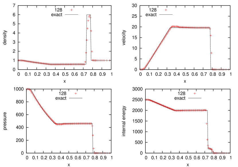
To test the behavior of the hydrodynamics solver, we run several different 1D shock tube problems. The setup for these problems consists of a left and right state, with the interface in the center of the domain. All calculations use a gamma-law equation of state with We show results from each problem run using 1D Cartesian coordinates, but we have verified that the results are identical when each problem is run in 2D or 3D Cartesian coordinates and the interface is normal to a coordinate axis. The length of the domain is always taken as 1.0, with the interface in the center. We use a base grid of 32 cells, with two additional levels of factor 2 refinement, for an effective resolution of 128 cells. The refinement criteria are based on gradients of density and velocity. In the case of the double rarefaction we also present results from runs with two levels of factor 4 refinement (effective resolution of 512 cells) and three levels of factor 4 refinement (effective resolution of 2048 cells). In each case, analytic solutions are found using the exact Riemann solver from Toro (1997). All calculations are run with the new PPM limiters and a CFL number of 0.9. For each problem we show density, pressure, velocity, and internal energy.
8.1.1 Sod’s Problem
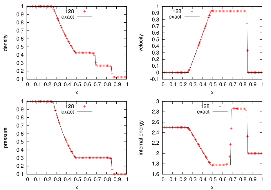
The Sod problem (Sod, 1978) is a simple shock tube problem that exhibits a shock, contact discontinuity, and a rarefaction wave. The non-dimensionalized initial conditions are:
| (41) |
This results in a rightward moving shock and contact discontinuity, and a leftward moving rarefaction wave. Figure 3 shows the resulting pressure, density, velocity, and internal energy at s. We see excellent agreement with the exact solution.
8.1.2 Double Rarefaction
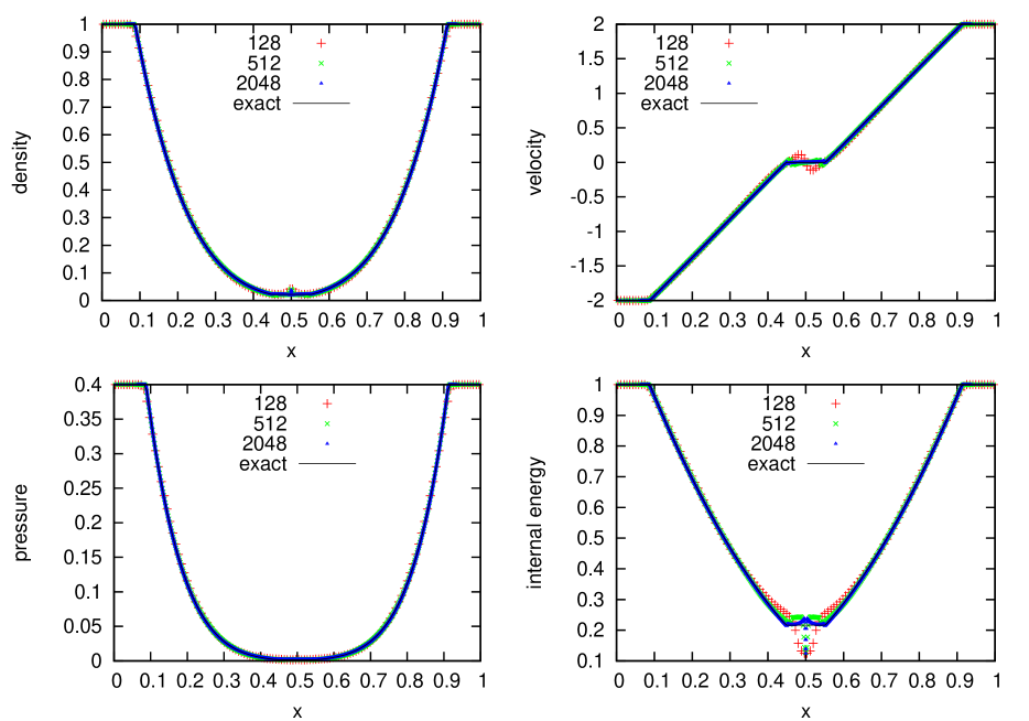
The double rarefaction problem tests the behavior of the hydrodynamics algorithm in regions where a vacuum is created. We run the problem as described in Toro (1997). The non-dimensionalized initial conditions are:
| (42) |
This results in two rarefaction waves propagating in opposite directions away from the center. As a result, matter is evacuated from the center, leaving behind a vacuum. Figure 4 shows the CASTRO solutions at s. The agreement with the exact solution is excellent at the 128-cell resolution for density, pressure and velocity; the internal energy is more sensitive, but clearly converges to the analytic solution except at the center line. This is a very common pathology for this problem, since the internal energy, , is derived from equation (7) using values of and which are both approaching zero in the center of the domain (Toro, 1997).
8.1.3 Strong Shock
The final shock-tube problem we try is a strong shock. We initialize the problem as described in Toro (1997). The initial conditions are:
| (43) |
The initial pressure jump of six orders of magnitude results in a strong rightward moving shock. This large dynamic range can cause trouble for some hydrodynamics solvers. The shock is followed very closely by a contact discontinuity. A leftward moving rarefaction is also present. Figure 5 shows the CASTRO results at s. We see good agreement between the CASTRO results and the exact solution.
8.2 Sedov
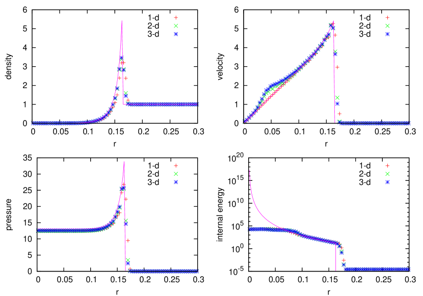
Another standard hydrodynamics test is the Sedov-Taylor blast wave. The problem setup is very simple: a large amount of energy is deposited into the center of a uniform domain. This drives a blast wave (spherical or cylindrical, depending on the domain geometry). An analytic solution is provided by Sedov (1959). We use a publicly available code described by Kamm & Timmes (2007) to generate the exact solutions.
The Sedov explosion can test the geometrical factors in the hydrodynamics scheme. A cylindrical blast wave (e.g. a point explosion in a 2D plane) can be modeled in 2D Cartesian coordinates. A spherical blast wave can be modeled in 1D spherical, 2D axisymmetric (cylindrical -), or 3D Cartesian coordinates.
In the Sedov problem, the explosion energy, (in units of energy, not energy/mass or energy/volume), is deposited into a single point, in a medium of uniform ambient density, , and pressure, . Initializing the problem can be difficult because the small volume is typically only one cell in extent, which can lead to grid imprinting in the solution. A standard approach (see for example Fryxell et al. 2000; Omang et al. 2006 and the references therein) is to convert the explosion energy into a pressure contained within a certain volume, , of radius as
| (44) |
This pressure is then initialized to in all of the cells where . We use the gamma-law equation of state with .
To further minimize any grid effects, we do subsampling in each cell: each cell is divided it into subcells in each coordinate direction, each subcell is initialized independently, and then the subcells are averaged together (using volume weighting for spherical or cylindrical coordinates) to determine the initial state of the full cell.
For these runs, we use , , , , and . A base grid with cm is used with three levels of factor 2 refinement. For most geometries, we model the explosion in a domain ranging from 0 to 1 cm in each coordinate direction. In this case, the base grid would have 32 cells in each coordinate direction and the finest mesh would correspond to 256 cells in each coordinate direction. For the 2D axisymmetric case, we model only one quadrant, and the domain ranges from 0 to 0.5 cm. All calculations were run with a CFL number of 0.5, and the initial time step was shrunk by a factor of 100 to allow the point explosion to develop. We refine on regions where , , , or .
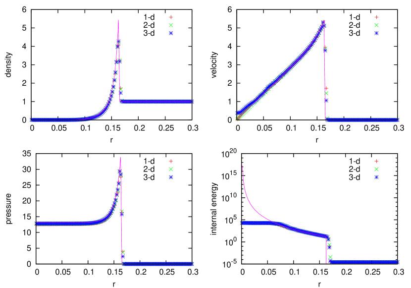
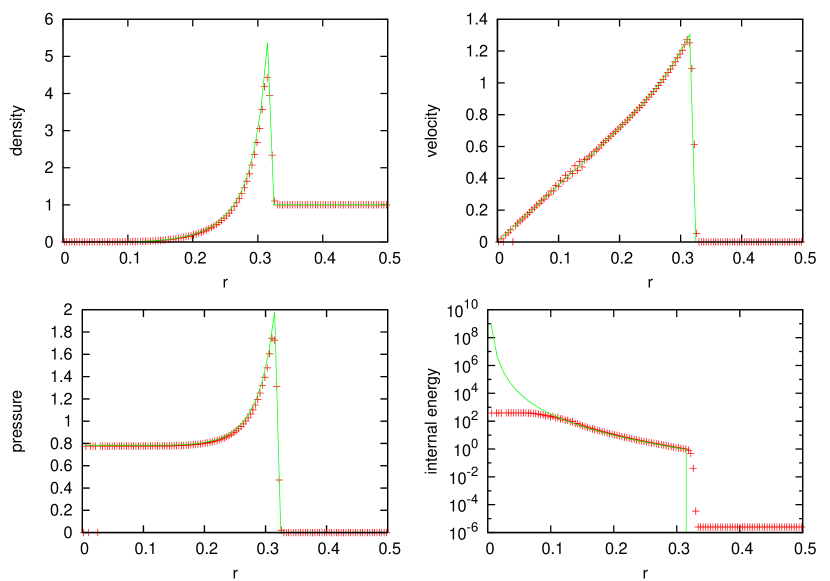
Figure 6 shows the CASTRO solution to a spherical Sedov explosion at time s, run in 1D spherical, 2D cylindrical, and 3D Cartesian coordinates. For the 2D and 3D solutions, we compute the radial profile by mapping each cell into its corresponding radial bin and averaging. The radial bin width was picked to match the width of a cell at the finest level of refinement in the CASTRO solution. The density, velocity, and pressure plots match the exact solution well. As with the double rarefaction problem, the internal energy is again the most difficult quantity to match due to the vacuum region created at the origin. Figure 7 shows the same set of calculations run with 4 levels of factor 2 refinement. Here the agreement is even better. Figure 8 shows the CASTRO solution at time s to a cylindrical Sedov explosion, run in 2D Cartesian coordinates.
8.3 Rayleigh-Taylor
The Rayleigh-Taylor instability results when a dense fluid is placed over a less-dense fluid in a gravitational field (Taylor, 1950; Layzer, 1955; Sharp, 1984). The interface is unstable and a small perturbation will result in the growth a buoyant uprising bubbles and dense, falling spikes of fluid. This instability provides a mechanism for mixing in many astrophysical systems. Despite its seemingly simplistic nature, only the linear growth regime is understood analytically (see for example Chandrasekhar 1961). In the non-linear regime, Rayleigh-Taylor instability calculations are often used as a means of code validation (Dimonte et al., 2004).
For our purposes, the R-T instability provides a good basis to compare different choices of the advection algorithm. We model a single-mode Rayleigh-Taylor instability—a perturbation consisting of a single wavelength that disturbs the initial interface. Short-wavelength perturbations have a faster growth rate than long-wavelength perturbations, so grid effects can easily drive the instability on smaller scales than our initial perturbation. No viscous terms are explicitly modeled.
We choose the density of the dense fluid to be and the light fluid is . The gravitational acceleration is taken to be in the vertical direction. The gamma-law equation of state is used with . Our domain has a width of cm and a height of cm. The initial interface separating the high and low density fluid is centered vertically at , with the density in the top half taken to be and the density in the lower half . Since and , are constant, we can analytically integrate the equation of hydrostatic equilibrium to get the pressure in both the high and low-density regions of the domain:
| (45) |
where is the vertical coordinate, and is the pressure at the base of the domain. We take .
To initiate the instability, the interface is perturbed by slightly shifting the density, keeping the interface centered vertically in the domain. We define the perturbed interface height, , to be a function of position in the -direction as
| (46) |
with the amplitude, cm. We note that the cosine part of the perturbation is done symmetrically, to prevent roundoff error from introducing an asymmetry in the flow. The density is then perturbed as:
| (47) |
The profile provides a slight smearing of the initial interface, over a smoothing length . We take cm.
In Figure 9, we present simulation results for the Rayleigh-Taylor problem at s for several different variants of the hydrodynamics. All calculations were run with grid cells. In the bottom right image we show the results obtained using the unsplit PPM with the new limiter used in CASTRO. The left and middle images on the bottom row are results using the unsplit piecewise linear method and unsplit PPM with limiters as in Miller & Colella (2002), respectively. The results with all three methods are reasonably good; however, the piecewise linear and original PPM limiter both exhibit mild anomalies at the tip of both the bubble and the spike.
In the upper row, we present results for the Rayleigh-Taylor problem using operator-split analogs of the unsplit methods. The details of the algorithms such as limiters, Riemann solver, etc. are the same as in the unsplit methods; the only difference is the use of operator splitting. We note that all three of the operator-split methods produce spurious secondary instabilities. This behavior is a direct result of the operator-split approach. Physically, for these low Mach number flows, the density field is advected by a nearly incompressible flow field, and remains essentially unchanged along Lagrangian trajectories. However, in regions where there is significant variation in the local strain rate, an operator-split integration approach alternately compresses and expands the fluid between subsequent sweeps. This alternating compression / expansion provides the seed for the anomalies observed with operator-split methods.
We note that both the CPU time and the memory usage are roughly a factor of two larger for the unsplit algorithm than for the split algorithm in this two-dimensional implementation. For a pure hydrodynamics problem with gamma-law equation of state this factor is nontrivial; for a simulation that uses the full self-gravity solver, a realistic reaction network, a costly equation of state, or significant additional physics, the additional cost of the hydrodynamic solver may be negligible.
In 3D one might expect the ratio of CPU time for the unsplit algorithm relative to the split algorithm to be be even larger than in 2D because of the additional Riemann solves required to construct the transverse terms. However, this effect is counterbalanced by the need to advance ghost cells in the split algorithm to provide boundary conditions for subsequent sweeps. Consequently, we observe an increase in CPU time that is slightly less than the factor of two observed in 2D. The 3D implementation of the unsplit algorithm in CASTRO uses a strip-mining approach that only stores extra data on a few planes at a time, so we see an increase of less than 10% in the memory required for the unsplit integrator compared to the split integrator in 3D.
8.4 Stationary Star Gravity
A challenging problem for a hydrodynamics code is to keep a star in hydrostatic equilibrium. Because of the different treatment of the pressure, density, and gravitational acceleration by the hydrodynamics algorithm, small motions can be driven by the inexact cancellation of and . This is further exaggerated by modeling a spherical star on a 3D Cartesian grid. Here we test the ability of CASTRO to maintain hydrostatic equilibrium for a spherical, self-gravitating star.
Our initial model is a nearly-Chandrasekhar mass, carbon-oxygen white dwarf, which is generated by specifying a core density (), temperature ( K), and a uniform composition () and integrating the equation of hydrostatic equilibrium outward while constraining the specific entropy, , to be constant. In discrete form, we solve:
| (48) | |||||
| (49) |
with cm. We begin with a guess of and and use the equation of state and Newton-Raphson iterations to find the values that satisfy our system. Since this is a spherical, self-gravitating star, the gravitation acceleration, , is updated each iteration based on the current value of the density. Once the temperature falls below K, we keep the temperature constant, and continue determining the density via hydrostatic equilibrium until the density falls to , after which we hold the density constant. This uniquely determines the initial model. We note that this is the same procedure we follow to initialize a convecting white dwarf for the multilevel low Mach number code, MAESTRO, described in Nonaka et al. (2010).
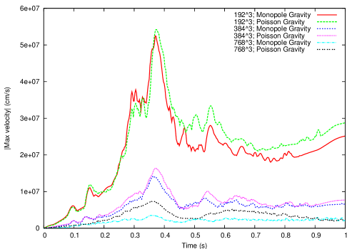
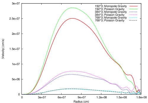
We map the model onto a ( cm)3 domain with 1923, 3843, and 7683 grid cells, and center the star in the domain. We let the simulation run to 1 s, and compare the maximum magnitude of velocity vs. time and the magnitude of velocity vs. radius at s, a time greater than two sound-crossing times. We only consider regions of the star at cm, which corresponds to a density of . Note that the density reaches the floor of 10 at cm. We turn on the sponge at the radius where and the sponge reaches its full strength at the radius where with a sponge strength of . We use a CFL of 0.9 and no refinement. We use the Helmholtz equation of state (Timmes & Swesty, 2000; Fryxell et al., 2000) and no reactions are modeled.
Figure 10 shows a plot of the maximum magnitude of velocity vs. time. At each of the three resolutions, we show the results using a monopole gravity approximation and Poisson solve for gravity. We note that in each simulation, the maximum velocity is not strictly increasing, leading us to believe that over longer periods of time the velocities will remain small. We note that sound speed at the center of the star is approximately cm/s, so at the highest resolution, the peak velocity is less than 1% of the sound speed. The monopole and Poisson cases match up very well, except for the finest resolution. The reason why we see larger peak velocities in the finest resolution Poisson solver simulation is due to the large velocities at the edge of the star.
Figure 11 shows a plot of the magnitude of velocity vs. radius at s. Again, at each of the three resolutions, we show the results using a monopole gravity approximation and Poisson solve for gravity. Here, we see clear second order convergence in the max norm, and the monopole and Poisson simulations agree best at the highest resolution. We also see how in the finest resolution runs, the velocities at the edge of the star can become large, but this is likely outside the region of interest for a typical simulation.
8.5 Homologous Dust Collapse
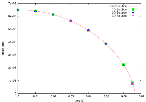
As a second test of the gravity solver in CASTRO we implement the homologous dust collapse test problem, a ‘pressure-less’ configuration that collapses under its own self-gravity. An analytic solution that describes the radius of the sphere as a function of time is found in Colgate & White (1966). Our implementation of this problem follows that described in FLASH 3.2 User’s Guide (2009); Monchmeyer & Muller (1989). The problem is initialized with a sphere with a large, uniform density, , of radius . The pressure everywhere should be negligible, i.e., the sound crossing time should be much longer than the free-fall collapse time (see, for example, FLASH 3.2 User’s Guide 2009). Colgate & White (1966) use . We choose a value that does not appear to affect the dynamics. As the sphere collapses, the density inside should remain spatially constant, but increase in value with time.
Following FLASH 3.2 User’s Guide (2009), we take and . The pressure is not specified, so we take it to be dyn cm Outside of the sphere, we set the density to . Finally, since the sharp cutoff at the edge of the sphere is unphysical, we smooth the initial profile by setting
| (50) |
with the smoothing length, . We use the gamma-law equation of state with .
Figure 12 shows the radius vs. time for the 1D, 2D, and 3D simulations as compared to the exact solution. In all three cases we see excellent agreement with the exact solution.
8.6 Reacting Bubbles in a Stellar Atmosphere
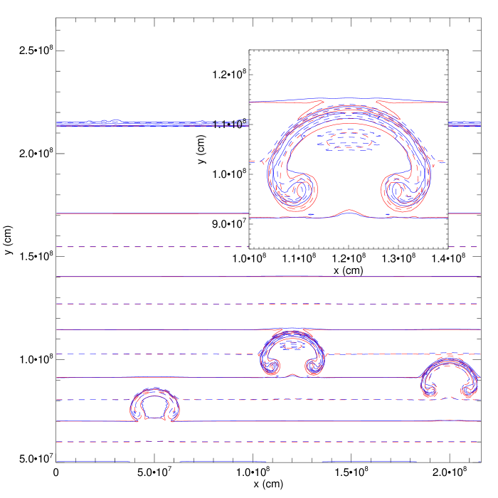
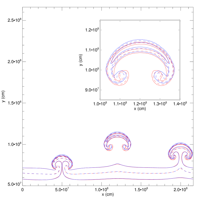
A final test is a code comparison of the evolution of three reacting bubbles in a plane-parallel stellar atmosphere. This problem is almost identical to the setup described in Section 4.2 of Almgren et al. (2008) with two minor differences. First, we eliminate the stably stratified layer at the base of the atmosphere by setting the lower extrema of the domain to cm—this way, the bottommost row of cells in the domain is initialized with the specified base density () and temperature. Second, we set the base temperature of the atmosphere to K (instead of K) to minimize the amount of reactions occurring near the lower domain boundary. Three temperature perturbations are seeded in pressure-equilibrium with a range of heights and widths as specified by equation (87) and Table 1 of Almgren et al. (2008). We use a uniform computation grid of cells and a domain width of cm.
We compare the evolution to the FLASH code (Fryxell et al., 2000), version 2.5, using the standard dimensionally-split PPM hydrodynamics module that comes with FLASH. The lower boundary condition in both cases provides hydrostatic support by integrating the equation of hydrostatic equilibrium together with the equations of state into the ghost cells, assuming a constant temperature, as described in Zingale et al. (2002). The left and right boundary is periodic. We use the same single step () reaction module described in Almgren et al. (2008). Both codes use the general stellar equation of state described in Fryxell et al. (2000); Timmes & Swesty (2000) with the Coulomb corrections enabled.
8.7 Type Ia Supernova
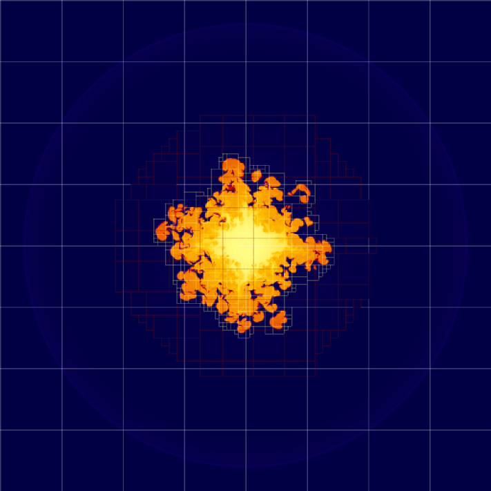
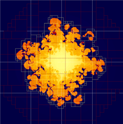
As a final example, in Figure 15 we show a 2D snapshot of temperature from a 3D calculation of a Type Ia supernova (Ma & Aspden, 2010; Ma et al., 2010). This simulation uses a realistic stellar equation of state and a turbulent flame model, and is typical of more realistic CASTRO applications. The domain is 5.12 x cm on a side, and is covered with 512 grids. There are two levels of factor two refinement, with approximately 1.8% of the domain covered by level 2 grids with an effective resolution of 2.5 x cm. Figure 16 is a close-up of the center of the domain so that the level 2 grids are more visible.
9 Summary
We have described a new Eulerian adaptive mesh code, CASTRO, for solving the multicomponent compressible hydrodynamic equations with a general equation of state for astrophysical flows. CASTRO differs from existing codes of its type in that it uses unsplit PPM for its hydrodynamic evolution, subcycling in time, and a nested hierarchy of logically-rectangular grids. Additional physics includes self-gravitation, nuclear reactions, and radiation. Radiation will be described in detail in the next paper, Part II, of this series.
CASTRO is currently being used in simulations of Type Ia supernovae and core-collapse supernovae; examples of simulations done using CASTRO can be found in Joggerst et al. (2009); Woosley et al. (2009). Further details on the CASTRO algorithm can be found in the CASTRO User Guide (CASTRO User Guide, 2009).
References
- Almgren et al. (1998) Almgren, A. S., Bell, J. B., Colella, P., Howell, L. H., & Welcome, M. L. 1998, Journal of Computational Physics, 142, 1
- Almgren et al. (2008) Almgren, A. S., Bell, J. B., Nonaka, A., & Zingale, M. 2008, Astrophysical Journal, 684, 449
- Bell et al. (1994) Bell, J., Berger, M., Saltzman, J., & Welcome, M. 1994, SIAM J. Sci. Statist. Comput., 15, 127
- Bell et al. (1989) Bell, J. B., Colella, P., & Trangenstein, J. A. 1989, Journal of Computational Physics, 82, 362
- Berger & Colella (1989) Berger, M. J., & Colella, P. 1989, Journal of Computational Physics, 82, 64
- Berger & Oliger (1984) Berger, M. J., & Oliger, J. 1984, Journal of Computational Physics, 53, 484
- Berger & Rigoutsos (1991) Berger, M. J., & Rigoutsos, J. 1991, IEEESMC, 21, 1278
- Bryan et al. (1995) Bryan, G. L., Norman, M. L., Stone, J. M., Cen, R., & Ostriker, J. P. 1995, Computer Physics Communications, 89, 149
- CASTRO User Guide (2009) CASTRO User Guide. 2009, https:ccse.lbl.gov/Research/CASTRO/CastroUserGuide.pdf
- Chandrasekhar (1961) Chandrasekhar, S. 1961, Hydrodynamic and hydromagnetic stability, ed. S. Chandrasekhar, dover reprint, 1981
- Colella (1990) Colella, P. 1990, Journal of Computational Physics, 87, 171
- Colella & Glaz (1985) Colella, P., & Glaz, H. M. 1985, Journal of Computational Physics, 59, 264
- Colella et al. (1997) Colella, P., Glaz, H. M., & Ferguson, R. E. 1997, unpublished manuscript
- Colella & Sekora (2008) Colella, P., & Sekora, M. D. 2008, Journal of Computational Physics, 227, 7069
- Colella & Woodward (1984) Colella, P., & Woodward, P. R. 1984, Journal of Computational Physics, 54, 174
- Colgate & White (1966) Colgate, S. A., & White, R. H. 1966, ApJ, 143, 626
- Crutchfield (1991) Crutchfield, W. Y. 1991, Load Balancing Irregular Algorithms, Tech. Rep. UCRL-JC-107679, LLNL
- Dimonte et al. (2004) Dimonte, G. et al. 2004, Physics of Fluids, 16, 1668
- FLASH 3.2 User’s Guide (2009) FLASH 3.2 User’s Guide. 2009, http://flash.uchicago.edu/website/codesupport/
- Franklin Performance Monitoring (2010) Franklin Performance Monitoring. 2010, N5 IOR Aggregate Write, http://www.nersc.gov/nusers/systems/franklin/monitor.php
- Fryxell et al. (2000) Fryxell, B. et al. 2000, Astrophysical Journal Supplement, 131, 273
- Gittings et al. (2008) Gittings, M. et al. 2008, Computational Science and Discovery, 1, 015005
- Joggerst et al. (2009) Joggerst, C. C., Almgren, A., Bell, J., Heger, A., Whalen, D., & Woosley, S. E. 2009, Astrophysical Journal
- Kamm & Timmes (2007) Kamm, J. R., & Timmes, F. X. 2007, submitted to ApJ supplement, May 2007, see http://cococubed.asu.edu/code_pages/sedov.shtml
- Lattimer & Swesty (1991) Lattimer, J. M., & Swesty, F. D. 1991, Nuclear Physics A, 535, 331, code obtained from http://www.astro.sunysb.edu/dswesty/lseos.html
- Layzer (1955) Layzer, D. 1955, ApJ, 122, 1
- Ma & Aspden (2010) Ma, H., & Aspden, A. J. 2010, Private communication
- Ma et al. (2010) Ma, H., Woosley, S., Almgren, A., & Bell, J. 2010, in American Astronomical Society Meeting Abstracts, Vol. 215, American Astronomical Society Meeting Abstracts, 343.01–+
- McCorquodale & Colella (2010) McCorquodale, P., & Colella, P. 2010, Journal of Computational Physics, to appear
- Miller & Colella (2002) Miller, G. H., & Colella, P. 2002, Journal of Computational Physics, 183, 26
- Miniati & Colella (2007) Miniati, F., & Colella, P. 2007, Journal of Computational Physics, 227, 400
- Monchmeyer & Muller (1989) Monchmeyer, R., & Muller, E. 1989, A&A, 217, 351
- Müller (1986) Müller, E. 1986, A&A, 162, 103
- Nonaka et al. (2010) Nonaka, A., Almgren, A. S., Bell, J. B., Lijewski, M. J., Malone, C., & Zingale, M. 2010, ApJS, submitted
- Omang et al. (2006) Omang, M., Børve, S., & Trulsen, J. 2006, Journal of Computational Physics, 213, 391
- O’Shea et al. (2005) O’Shea, B. W., Bryan, G., Bordner, J., Norman, M. L., Abel, T., Harkness, R., & Kritsuk, A. 2005, in Lecture Notes in Computational Science and Engineering, Vol. 41, Adaptive Mesh Refinement – Theory and Applications, ed. T. Plewa, T. Linde, & V. G. Weirs (Springer), 341–350
- Plewa & Müller (1999) Plewa, T., & Müller, E. 1999, Astronomy and Astrophysics, 342, 179
- Rendleman et al. (2000) Rendleman, C. A., Beckner, V. E., Lijewski, M., Crutchfield, W. Y., & Bell, J. B. 2000, Computing and Visualization in Science, 3, 147
- Ricker (2008) Ricker, P. M. 2008, ApJS, 176, 293
- Saltzman (1994) Saltzman, J. 1994, Journal of Computational Physics, 115, 153
- Sedov (1959) Sedov, L. I. 1959, Similarity and Dimensional Methods in Mechanics (Academic Press), translated from the 4th Russian Ed.
- Sharp (1984) Sharp, D. H. 1984, Physica D Nonlinear Phenomena, 12, 3
- Sod (1978) Sod, G. A. 1978, Journal of Computational Physics, 27, 1
- Strang (1968) Strang, G. 1968, SIAM J. Numerical Analysis, 5, 506
- Taylor (1950) Taylor, G. 1950, Royal Society of London Proceedings Series A, 201, 192
- Timmes & Swesty (2000) Timmes, F. X., & Swesty, F. D. 2000, Astrophysical Journal Supplement, 126, 501
- Toro (1997) Toro, E. F. 1997, Riemann Solvers and Numerical Methods for Fluid Dynamics (Springer)
- VisIt User’s Manual (2005) VisIt User’s Manual. 2005, https://wci.llnl.gov/codes/visit/home.html
- Woosley et al. (2009) Woosley, S. E. et al. 2009, Journal of Physics Conference Series, 180, 012023
- Zingale et al. (2009) Zingale, M., Almgren, A. S., Bell, J. B., Nonaka, A., & Woosley, S. E. 2009, Astrophysical Journal, 704, 196
- Zingale et al. (2002) Zingale, M. et al. 2002, Astrophysical Journal Supplement, 143, 539
