Rotational effects in thermonuclear type I bursts: equatorial crossing and directionality of flame spreading

Abstract

In a previous study on thermonuclear (type I) bursts on accreting neutron stars we addressed and demonstrated the importance of the effects of rotation, through the Coriolis force, on the propagation of the burning flame. However, that study only analysed cases of longitudinal propagation, where the Coriolis force coefficient $2\Omega\cos\theta$ was constant. In this paper, we study the effects of rotation on propagation in the meridional (latitudinal) direction, where the Coriolis force changes from its maximum at the poles to zero at the equator. We find that the zero Coriolis force at the equator, while affecting the structure of the flame, does not prevent its propagation from one hemisphere to another. We also observe structural differences between the flame propagating towards the equator and that propagating towards the pole, the second being faster. In the light of the recent discovery of the low spin frequency of burster IGR J17480-2446 rotating at 11 Hz (for which Coriolis effects should be negligible) we also extend our simulations to slow rotation.

1 Introduction

Type I bursts are a phenomenon measured in more than 100 accreting Neutron Stars (NSs) in low mass X-ray binaries (see MINBAR at http://burst.sci.monash.edu/minbar, Galloway et al., 2010). During the bursts the matter accreted by the NS burns unstably after reaching the critical column density (see e.g. Fujimoto et al., 1981). The time scales for different bursts can vary, but in general they last from tens to hundreds of seconds depending on different factors like the reactions taking place, the ignition depth, the diffusion of photons through the non-burning layers and the propagation of the flame across the surface (see for example Lewin et al., 1993; Strohmayer & Bildsten, 2006, for reviews).

Flame propagation during type I bursts is an essential component of burst dynamics. Even if the accreted material is more or less homogeneously distributed, it would be improbable that it would ignite simultaneously everywhere on the surface (Bildsten, 1995). After ignition is triggered at one location, flame propagation is important to understand the observations of the rise of the lightcurve, but there is more: NS parameters, like mass and radius, could be derived from the lightcurves (see, e.g. Güver et al., 2010; Steiner et al., 2010; Suleimanov et al., 2011; Zamfir et al., 2012; Miller, 2013, for a recent review) and whether the flame is burning across the full surface or only on one hemisphere, could have implications on the inferred parameters.

Previously, Spitkovsky et al. (2002) employed analytical arguments and shallow water numerical simulations to demonstrate the defining role of rotation on the flame structure. Recently, Cavecchi et al. (2013) presented vertically resolved simulations of propagating deflagrations in rotating oceans on the surface of NSs; they analysed the effects of rotation by means of 2D numerical hydrodynamics simulations, using a code described in Braithwaite & Cavecchi (2012) and its modifications in Cavecchi et al. (2013). The main conclusions of the latter paper were twofold. First, in the presence of rotation the fluid is not free to move, so that, after ignition, it expands vertically and tries to spill over sideways on to the cold fluid. However, the Coriolis force prevents such motion, diverting the fluid in the perpendicular direction and creating hurricanes of fire that extend to two to three Rossby radii $R_{\rm Ro}=\sqrt{(}gH)/2\Omega$ (where $g$ is the gravitational acceleration at the surface of the NS, $H$ the scale height of the fluid and $\Omega$ the angular velocity of the star). In this way the interface between the hot and cold fluid, the flame front, where most of the burning is happening, is along a line inclined at an angle $\sim H/R_{\rm Ro}$: this is in agreement with what Spitkovsky et al. (2002) proposed. Secondly, inspection of the simulations revealed that the main driver of the propagation, what makes the cold fluid ignite, is the conduction across the front (helped by fluid motion induced by the baroclinicity at the hot-cold fluid interface). Therefore, the speed is proportional to the thermal conductivity, $1/\kappa_{\rm{c}}$, where $\kappa_{\rm{c}}$ is the opacity of the fluid. The timescales for conduction are slow, but the front is not vertical, it is inclined as mentioned above, therefore there is a geometrical factor, given by the inverse of the inclination angle, of the order of $R_{\rm Ro}/H$ that speeds up the propagation bringing it to values comparable to observations (Cavecchi et al., 2013). This relation implied that the speed of the flame should be proportional to the Rossby radius and therefore to $1/\Omega$.

However, Cavecchi et al. (2013) considered only longitudinal propagation, using a constant value of the Coriolis parameter for each run. Smaller values of the spin exhibited faster propagation, but also less confinement. This raised a very interesting question. Near the equator, the Coriolis force vanishes and consequently so does the confinement of the fluid. Could this prevent the propagation of the fluid from one hemisphere to the other by quenching the flame? We address this question in this paper.

For this work, while keeping the 2D setup, we have added the possibility for the Coriolis parameter to vary with a cosine dependence on the horizontal coordinate in order to mimic the variation of the Coriolis force with latitude and analysed the behaviour of the flame while approaching the equator. The structure of this paper is the following: in the next section we report the results of our simulations regarding meridional propagation and in Section 3 we draw our conclusions.

2 Meridional propagation

In Cavecchi et al. (2013) the question was raised whether a flame igniting somewhere in one hemisphere could cross the equator and reach the other hemisphere. The concern was that since the Coriolis force vanishes at the equator, it would no longer be able to balance the horizontal pressure gradient during the crossing, and the deflagration would become de-confined and would fizzle out. This section is devoted to the study of the flame propagation with non-constant Coriolis parameter that goes to zero and switches sign in the middle of our computational domain, but first we describe some necessary changes to the code and the caveats.

2.1 Equations of motions

Cast in spherical coordinates, with $r$ along the outgoing radial direction, $\varphi$ increasing from west to east and $\theta$ going from north to south, the north being defined by the positive direction of the rotation axis, the equations of motion read:

$$\frac{\rm{D}{U^{\rm r}}}{\rm{D}t}-\frac{{U^{\theta}}^{2}+{U^{\varphi}}^{2}}{r}= 2\Omega\sin\theta{U^{\varphi}}-\frac{1}{\rho}\frac{\partial P}{\partial r}+\frac{\partial\tilde{\phi}}{\partial r}+\frac{{F^{\rm r}}}{\rho}$$ (1)

$$\frac{\rm{D}{U^{\varphi}}}{\rm{D}t}+\frac{{U^{\rm r}}{U^{\varphi}}}{r}+\frac{{U^{\theta}}{U^{\varphi}}}{r\tan\theta}= -2\Omega\cos\theta{U^{\theta}}-2\Omega\sin\theta{U^{\rm r}}+$$

$$-\frac{1}{\rho}\frac{1}{r\sin\theta}\frac{\partial P}{\partial\varphi}+\frac{1}{r\sin\theta}\frac{\partial\tilde{\phi}}{\partial\varphi}+\frac{{F^{\varphi}}}{\rho}$$ (2)

$$\frac{\rm{D}{U^{\theta}}}{\rm{D}t}+\frac{{U^{\rm r}}{U^{\theta}}}{r}-\frac{{U^{\varphi}}^{2}}{r\tan\theta}= 2\Omega\cos\theta{U^{\varphi}}-\frac{1}{\rho}\frac{1}{r}\frac{\partial P}{\partial\theta}+\frac{1}{r}\frac{\partial\tilde{\phi}}{\partial\theta}+\frac{{F^{\theta}}}{\rho}$$ (3)

$$\frac{\rm{D}\rho}{\rm{D}t}=-\rho\left\{\frac{\partial{U^{\rm r}}}{\partial r}+\frac{1}{\rho}\frac{1}{r\sin\theta}\right. \left.\frac{\partial{U^{\varphi}}}{\partial\varphi}+\frac{1}{r}\frac{\partial{U^{\theta}}}{\partial\theta}+\frac{2{U^{\rm r}}}{r}+\frac{{U^{\theta}}}{r\tan\theta}\right\}$$ (4)

Where $\rm{D}/\rm{D}t$ expresses the total derivative

$$\frac{\rm{D}}{\rm{D}t}=\frac{\partial}{\partial t}+{U^{\rm r}}\frac{\partial}{\partial r}+{U^{\varphi}}\frac{1}{r\sin\theta}\frac{\partial}{\partial\varphi}+{U^{\theta}}\frac{1}{r}\frac{\partial}{\partial\theta},$$ (5)

and the three velocities are ${U^{\rm r}}=\dot{r}$, ${U^{\varphi}}=r\sin\theta\dot{\varphi}$, ${U^{\theta}}=r\dot{\theta}$. $\Omega$ is the angular velocity, and $\tilde{\phi}=-gr+\Omega^{2}r^{2}\sin^{2}\theta/2$ is the potential corrected for the centrifugal forces. ${F^{*}}$ are the viscous forces per unit volume.

The form of $\tilde{\phi}$ clearly shows that the coordinate surfaces $r=\rm{const}$ are not potential surfaces anymore and this results in a component of the potential force in the horizontal direction. However, as is customary in geophysical sciences (White et al., 2005), if we are interested in a thin layer whose mass is not contributing significantly to the gravitational force, we can approximate the potential surfaces to spheres and also drop any curvature term not proportional to $1/\tan\theta$. In doing so, we set $r=R_{\rm S}+x$, with $R_{\rm S}\gg x$, so that we can approximate $r$ to $R_{\rm S}$, apart from where differentiation is involved, and $\tilde{\phi}=-gx$, where we safely remove the constant $-gR_{\rm S}$ from the potential (the dependence of the potential on the colatitude should not be present, otherwise fake vorticity is introduced, see White et al., 2005); finally, we can reduce the $r$ component of the momentum equation to the hydrostatic equilibrium one. In summary we have:

$$\frac{1}{\rho}\frac{\partial P}{\partial x}= \frac{\partial\tilde{\phi}}{\partial x}$$ (6)

$$\frac{\rm{D}{U^{\varphi}}}{\rm{D}t}+\frac{{U^{\theta}}{U^{\varphi}}}{R_{\rm S}\tan\theta}= -2\Omega\cos\theta{U^{\theta}}-\frac{1}{\rho}\frac{1}{R_{\rm S}\sin\theta}\frac{\partial P}{\partial\varphi}+$$

$$+\frac{1}{R_{\rm S}\sin\theta}\frac{\partial\tilde{\phi}}{\partial\varphi}+\frac{{F^{\varphi}}}{\rho}$$ (7)

$$\frac{\rm{D}{U^{\theta}}}{\rm{D}t}-\frac{{U^{\varphi}}^{2}}{R_{\rm S}\tan\theta}= 2\Omega\cos\theta{U^{\varphi}}-\frac{1}{\rho}\frac{1}{R_{\rm S}}\frac{\partial P}{\partial\theta}+\frac{1}{R_{\rm S}}\frac{\partial\tilde{\phi}}{\partial\theta}+\frac{{F^{\theta}}}{\rho}$$ (8)

$$\frac{\rm{D}\rho}{\rm{D}t}=-\rho\left\{\frac{\partial{U^{\rm r}}}{\partial x}+\right. \left.\frac{1}{R_{\rm S}\sin\theta}\frac{\partial{U^{\varphi}}}{\partial\varphi}+\frac{1}{R_{\rm S}}\frac{\partial{U^{\theta}}}{\partial\theta}+\frac{{U^{\theta}}}{R_{\rm S}\tan\theta}\right\}$$ (9)

with

$$\frac{\rm{D}}{\rm{D}t}=\frac{\partial}{\partial t}+{U^{\rm r}}\frac{\partial}{\partial x}+{U^{\varphi}}\frac{1}{R_{\rm S}\sin\theta}\frac{\partial}{\partial\varphi}+{U^{\theta}}\frac{1}{R_{\rm S}}\frac{\partial}{\partial\theta}$$ (10)

The error in these expressions is then of order the eccentricity squared $e^{2}$ or the angular velocity measured in units of the (Newtonian) break-up velocity $\mu$ (van der Toorn & Zimmerman, 2008, $e=\sqrt{a^{2}-b^{2}}/a$, $\mu=a^{3}\Omega^{2}/G/M$, where $a$ and $b$ are the major and minor axis of the ellipsoid which would better approximate the star). An approximate estimation of $e$ and $\mu$ can be derived following Morsink et al. (2007). They present interpolating formulae to estimate $b$ (their $R(0)$) given the mass $M$, the radius $R_{\rm S}$ (their $R_{\rm eq}$) and $\Omega=2\pi\nu$. In this study, we use $M=1.4\rm{M_{\odot}}$ and $R_{\rm S}=(30/\pi)10^{5}$ cm; the spin frequency $\nu$ is at most $10^{3}$ Hz: in this case the maximum value for both $e$ and $\mu$ is $\sim 0.2$. Our reference case has $\nu=450$ Hz, with $e$ and $\mu$ $\sim 0.04$, resulting in an error of at most a few percent.

We use the hydrostatic numerical scheme described in Braithwaite & Cavecchi (2012), as modified in Cavecchi et al. (2013), and further include the terms that account for the spherical geometry. To do so, we change the vertical coordinate from $x$ to pressure $\sigma$. This is a hybrid coordinate system that relies on the hydrostatic approximation. $\sigma$ is defined in the following way: $P=\sigma P_{\ast}+P_{\rm{top}}$ with $P_{\ast}=P_{\rm{bot}}-P_{\rm{top}}$ (see Kasahara, 1974; Braithwaite & Cavecchi, 2012). In this coordinate system the upper boundary is fixed in pressure and the lower in space. $P_{\ast}$ is the pressure difference between bottom and top and changes as the fluid moves around. This system is well suited for NS oceans where the domain is much more extended horizontally than vertically and the hydrostatic assumption is justified; it also allows the grid to follow the vertical expansion of the fluid without the need for excessive memory (see Braithwaite & Cavecchi, 2012, for a more detailed discussion). After setting $R_{\rm S}\sin\theta{\rm{d}}\varphi={\rm{d}}y$, $R_{\rm S}{\rm{d}}\theta={\rm{d}}z$, ${U^{\rm r}}={U^{\rm x}}$, ${U^{\varphi}}=-{U^{\rm y}}$, ${U^{\theta}}={U^{\rm z}}$ and $\phi=-\tilde{\phi}=gx$ for convenience, our equations read

$$\frac{\partial\sigma}{\partial x}= -\frac{g\rho}{P_{\ast}}$$ (11)

$$\frac{\rm{D}{U^{\rm y}}}{\rm{D}t}+\frac{{U^{\rm z}}{U^{\rm y}}}{R_{\rm S}\tan\theta}= 2\Omega\cos\theta{U^{\rm z}}-\frac{\sigma}{\rho}\frac{\partial P_{\ast}}{\partial y}-\frac{\partial\phi}{\partial y}+\frac{{F^{\rm y}}}{\rho}$$ (12)

$$\frac{\rm{D}{U^{\rm z}}}{\rm{D}t}-\frac{{U^{\rm y}}^{2}}{R_{\rm S}\tan\theta}= -2\Omega\cos\theta{U^{\rm y}}-\frac{\sigma}{\rho}\frac{\partial P_{\ast}}{\partial z}-\frac{\partial\phi}{\partial z}+\frac{{F^{\rm z}}}{\rho}$$ (13)

$$\frac{\rm{D}\rho}{\rm{D}t}+\rho\left\{\frac{\partial\dot{\sigma}}{\partial\sigma}+\frac{\partial{U^{\rm y}}}{\partial y}\right.+ \left.\frac{\partial{U^{\rm z}}}{\partial z}+\frac{{U^{\rm z}}}{R_{\rm S}\tan\theta}\right\}=0$$ (14)

with

$$\frac{\rm{D}}{\rm{D}t}=\frac{\partial}{\partial t}+\dot{\sigma}\frac{\partial}{\partial\sigma}+{U^{\rm y}}\frac{\partial}{\partial y}+{U^{\rm z}}\frac{\partial}{\partial z}$$ (15)

and

$${\bm{\nabla}}_{\sigma}=\frac{\partial}{\partial y}+\frac{\partial}{\partial z}$$ (16)

Continuity Eq. (14) changes into an equation for $P_{\ast}$

$$\frac{\partial P_{\ast}}{\partial t}=-I_{\sigma=1}$$ (17)

with

$$I\equiv\int^{\sigma}_{0}\!\!\left({\bm{\nabla}}_{\sigma}\!\cdot\!(P_{\ast}{\bf U})+\frac{P_{\ast}{U^{\rm z}}}{R_{\rm S}\tan\theta}\right)\,{\rm d}\sigma^{\prime}$$ (18)

and

$$\dot{\sigma}=\frac{1}{P_{\ast}}\left(\sigma I_{\sigma=1}-I\right)$$ (19)

just as in Braithwaite & Cavecchi (2012), but with the new definition of $I$ with the extra term in $1/\tan\theta$ due to the use of spherical coordinates.

As for the energy equation, equation 11 in Cavecchi et al. (2013), it involves only scalar terms and they do not change, apart from the total derivative and the conduction term. As for this latter (Eq28 of Cavecchi et al., 2013) a similar treatment as above (see equation 3.17 of White et al., 2005, translating $a=R_{\rm S}$ and $\phi=\pi/2-\theta$) leads to

$$Q_{\rm{cond}}=\frac{1}{P_{\star}}\left\{{\bm{\nabla}}_{\sigma}\left[\frac{16\sigma_{B}T^{3}}{3\kappa_{\rm{c}}\rho}\left(\frac{P_{\star}}{\rho}{\bm{\nabla}}_{\sigma}T+{\bm{\nabla}}_{\sigma}\phi\frac{\partial T}{\partial\sigma}\right)\right]+\right.\\ +\frac{\partial}{\partial\sigma}\left[\frac{16\sigma_{B}T^{3}}{3\kappa_{\rm{c}}P_{\star}}\left({\bm{\nabla}}_{\sigma}\phi^{2}\frac{\partial T}{\partial\sigma}+\frac{P_{\star}}{\rho}{\bm{\nabla}}_{\sigma}\phi{\bm{\nabla}}_{\sigma}T\right.+\right.\\ \left.\left.\left.+g^{2}\frac{\partial T}{\partial\sigma}\right)\right]+\frac{16\sigma_{B}T^{3}}{3\kappa_{\rm{c}}\rho\tan\theta}\left(\frac{P_{\star}}{\rho}\frac{\partial T}{\partial z}+\frac{\partial\phi}{\partial z}\frac{\partial T}{\partial\sigma}\right)\right\}$$ (20)

where $\sigma_{\rm B}$ is the Stefan–Boltzmann constant and $\kappa_{\rm{c}}$ is the opacity, our parametrization of thermal conductivity, whose importance as the leading mechanism responsible for flame propagation was demonstrated in Cavecchi et al. (2013).

Thus, all our equations of motion look like those of Braithwaite & Cavecchi (2012) and Cavecchi et al. (2013). The only essential differences are the cosine dependence of the Coriolis force and the terms in $1/\tan\theta$. These we have implemented to simulate the variation of the Coriolis parameter from pole to pole and the effects of curvature.

A final remark regards the derivatives in the ‘$y$’ direction: this is the longitudinal direction and it is clear that dealing with it requires particular care, since we are dealing with circles of different length. As a first approximation we assume symmetry along the longitudinal direction, therefore setting to zero every derivative along $y$. The symmetry of our problems allows for such simplification: when igniting at the pole every longitude should be treated equally, while when igniting at the equator we are implying a ring ignition.

2.2 Initial setup

Name	$\kappa_{\rm{c}}$ [cm2 g-1]	$\nu$ [Hz]	$\delta$ [$10^{5}$ cm]
P1 / E1	$7\times 10^{-2}$	$10$	—
P2 / E2	$7\times 10^{-2}$	$100$	$6.03$
P3 / E3	$7\times 10^{-2}$	$450$	$2.77$
P4 / E4	$7\times 10^{-2}$	$1000$	$1.85$
P5 / E5	$7$	$450$	$2.77$
P6 / E6	$7\times 10^{-1}$	$450$	$2.77$
P7 / E7	$7\times 10^{-3}$	$450$	$2.77$

Table 1: Numerical parameters for the various simulations. $\kappa_{\rm{c}}$ is the opacity, $\nu$ is the spin frequency of the star. $\delta$ is the theoretical half width of the equatorial belt where the Coriolis force is not capable of confining the fluid. Simulations with $\nu=10$ Hz are not confined. All simulations have vertical resolution of $m_{\rm{x}}=96$. The horizontal resolution is $m_{\rm{z}}=480$ for the setups igniting at the pole (P) and it is $m_{\rm{z}}=240$ for those igniting at the equator (E).

We set up our simulations in a similar fashion to Cavecchi et al. (2013). In particular, the fluid is initially at rest and is made of pure helium, burning into carbon according to

$$Q_{\rm{n}}=5.3\times 10^{18}\rho_{5}^{2}\left(\frac{Y}{T_{9}}\right)^{3}e^{-4.4/T_{9}}\;\textrm{erg g${}^{-1}$ s${}^{-1}$},$$ (21)

where $T_{9}$ is temperature in units of $10^{9}$ K, $\rho_{5}$ is density in units of $10^{5}$ g cm^-3 and $Y$ is the mass fraction of helium. The temperature distribution is vertically constant with a horizontal dependence as:

$$T=T_{0}+\frac{\delta T}{1+\exp[(z-0.9\;\rm{km})/0.36\;\rm{km}]}$$ (22)

so that there is a greater temperature at one end of the domain, designed to ignite the fluid, whilst the distribution is flat in the rest of the domain, see Cavecchi et al. (2013) for details. Here we use $T_{0}=2\times 10^{8}$ K and $\delta T=2.81\times 10^{8}$ K. The lower value, $T_{0}=2\times 10^{8}$ K, is chosen to be neither too low, since the whole ocean must be close to ignition, nor so high as to trigger self ignition (see the ocean temperature profiles of Bildsten, 1995; Cumming & Bildsten, 2000, but note that the rate of energy production of the triple $\alpha$ reactions used by the latter authors is 1.9 times the rate used in this paper, since the authors apply this approximation to take carbon burning into account). The opacity $\kappa_{\rm{c}}$ is constant in each simulation, but different for different simulations (see Table 1 of this paper and the discussion at the end of section 2.2 of Cavecchi et al., 2013). The stellar spin $\nu$ varies between simulations from $10$ to $10^{3}$ Hz (see Table 1), while the surface gravity is $g=2\times 10^{14}$ cm s^-2. The horizontal length of the domain, the hemicircumference of the star, is $3\times 10^{6}$ cm, corresponding to $R_{\rm S}=(30/\pi)$ km, while in the vertical direction we include layers from $P_{\rm{top}}=10^{22}$ Pa to $P_{\rm{bot}}=e^{1.7}\times 10^{22}$ Pa. In the simulations for polar ignition the cosine term in the Coriolis force goes from $1$ to $-1$ across the domain. In the simulations for equatorial ignition, it goes from $0$ to $-1$.

The horizontal boundaries are symmetric in pressure difference $P_{\ast}$, temperature $T$ and composition. They are antisymmetric in the horizontal velocities. At the upper and lower boundaries, we use symmetric conditions for the temperature, composition and horizontal velocities. However, we include a cooling term, that affects the top of the simulation, based on an approximation of heat losses (see Cavecchi et al., 2013). We do not include any heat flux from the bottom boundary. In the case of equatorial ignition, the symmetry allows us to simulate just one hemisphere; simulations with polar ignition model the entire surface. We assume axisymmetry in both cases, thus limiting the simulations to 2D. The simulations have the same vertical resolution $m_{\rm{x}}=96$ grid points and horizontal resolutions of $m_{\rm{z}}=480$ for those that ignite at the pole and $m_{\rm{z}}=240$ for those igniting at the equator: that is equivalent to $6250$ cm in both cases. Artificial diffusivities are $\nu_{1}=0.03$ and $\nu_{2}=0.5$ (see Braithwaite & Cavecchi, 2012, for a description of the diffusion schemes implemented).

2.3 Polar ignition and equatorial crossing

Our key goal was to find out whether flames always crossed the equator, or whether the loss of Coriolis confinement led to quenching. We found that in every case we studied the fluid was eventually burning over the whole star. The simulations with the slowest rotation, $\nu=10$ Hz, were qualitatively different since the Rossby radius is larger than the star and no effective confinement is ever realized: this is discussed in more detail below (see Section 2.5). On the other hand, all the other runs developed a well defined flame front that crossed the equator in all cases.

Figure 1 shows the crossing of the equator for our reference run P3. The flame proceeds from the pole to the equator with a configuration similar to that described in Cavecchi et al. (2013) (see Figure 1, panel at $\approx 3.53$ s), the difference being a decreasing Coriolis force and increasing $R_{\rm Ro}$. This manifests itself as a flame front which is increasingly close to being horizontal and a speed up of flame propagation. When the flame is near enough to the equator, the Coriolis force is no longer able to significantly confine the hot fluid and this starts spilling over the cold fluid around the equator; the fluid is stopped in the Southern hemisphere once the Coriolis force is significant again (panel at $\approx 4.42$ s). As the burning layer on the other side is heating the layer below, the flame front is nearly horizontal. Thus, in the equatorial region the flame propagates vertically downwards (panels at $\approx 4.68$ - $\approx 4.94$ s). After consuming the equatorial belt the flame propagates in the Southern hemisphere (last panel of Figure 1, see also Section 2.4).

It is useful to define the equatorial belt as the region where the Coriolis force plays no essential dynamical role. Its extent is limited by the latitude on both sides of the equator where the distance to the equator is equal to the Rossby radius $R_{\rm Ro}=\sqrt{gH}/2\Omega\cos\theta$ at that point (and symmetrically on the other side):

$$z-\frac{\pi}{2}R_{\rm S}=\frac{\sqrt{gH}}{2\Omega\cos(z/R_{\rm S})}$$ (23)

The solutions to Eq. (23) can be transformed to the belt half width, $\delta=z-\frac{\pi}{2}R_{\rm S}$. Theoretical belt widths for each simulation are reported in Table 1 and drawn on Figures 1 - 3 and 5 for comparison with the results. Simulations with $\nu=10$ Hz do not have a belt width, in the sense that Eq. (23) does not have a meaningful solution since the Rossby radius is bigger than the star.

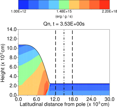
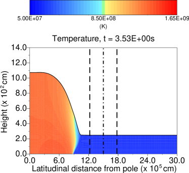
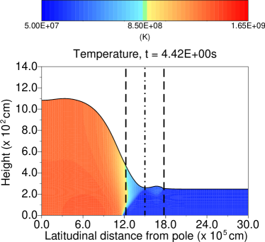
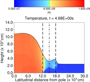
a) b)
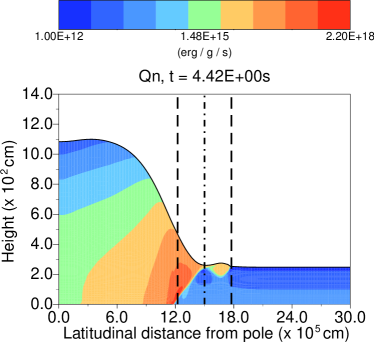
c) d)
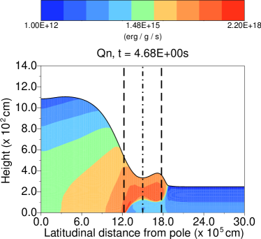
e) f)

Figure 1: The crossing of equator of P3 ($\nu=450$ Hz, $\kappa_{\rm{c}}=7\times 10^{-2}$ cm² g^-1). Heating rate due to nuclear burning, $Q_{\rm n}/{\tilde{c}_{\rm P}}$ as in equation 23 of Cavecchi et al., (2013), scaled by the gas constant value to make it in erg g^-1 s^-1 (left-hand column, logarithmic scale)${}^{\ref{note:units}}$ and temperature (right-hand column, linear scale). Vertical lines indicate the equator (dash dotted) and the belt (dashed, see Eq 23). The flame propagates confined by the Coriolis force in the Northern hemisphere. When it reaches the belt, confinement is not enough and the hot fluid begins spilling over the cold one. At the southern extreme of the belt Coriolis force is effective again and the fluid is confined again.

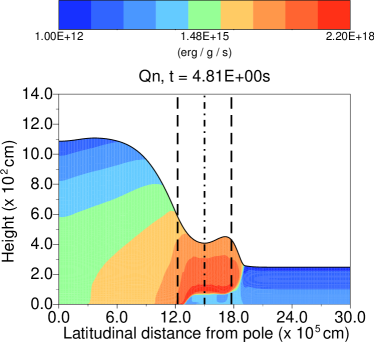
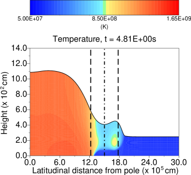
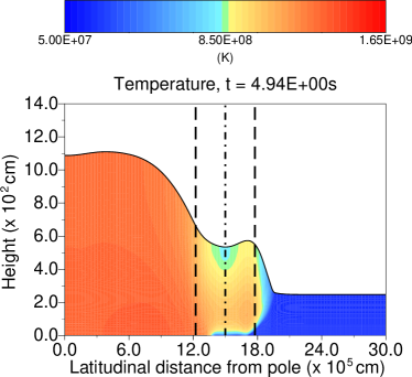
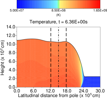
g) h)
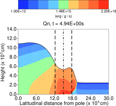
i) j)
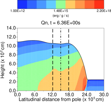
k) l)

Figure 1: Continued. The crossing of the equator of P3: the flame burns with a horizontal front and eventually continues the propagation in the Southern hemisphere being confined again.

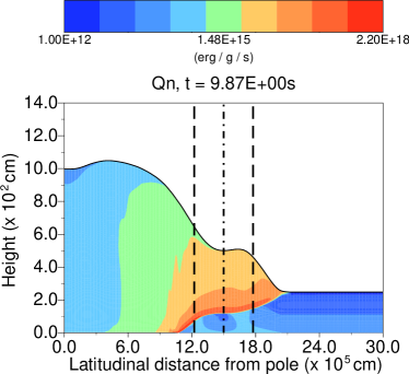
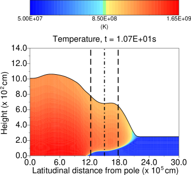
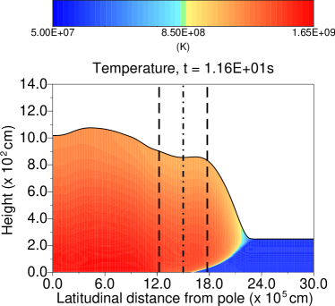
a) b)
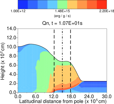
c) d)
e) f)

Figure 2: The crossing of equator of P5 ($\nu=450$ Hz, $\kappa_{\rm{c}}=7$ cm² g^-1). Same as Figure 1. The flame begins propagation in the Southern hemisphere before having reached the bottom of the simulation because of the higher opacity.

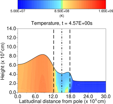
Figure 3: The crossing of equator of P7 ($\nu=450$ Hz, $\kappa_{\rm{c}}=7\times 10^{-3}$ cm² g^-1). Only the temperature profile is plotted. Vertical lines indicate the equator (dash dotted) and the belt (dashed, see Eq 23).

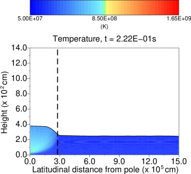
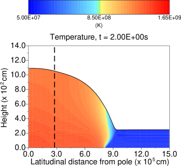
Figure 4: The ignition and propagation of the flame of E3. Same as Figure 3. Apart from an initial transitional stage, the propagation is identical to the southern propagation of simulation P3.

The behaviour of simulations P2, $\nu=10^{2}$ Hz, and P4, $\nu=10^{3}$ Hz, are qualitatively similar, the only difference being the variation in the Coriolis force confinement with $1/\nu$ dependence on spin frequency. Changing the thermal conductivity makes a greater qualitative impact on the flame’s dynamics, In Figure 2 we show for comparison the crossing of the equator in run P5, where the conductivity is much lower. As before, around the equator, the flame front is almost horizontal and ignition propagates vertically (first two panels of Figure 2). However, in this case, the vertical propagation is slow enough that the flame passes the equatorial belt before it has reached the bottom of the simulation. Note that temperature contours are more horizontal than in the case of P3. On the other hand, Figure 3 shows the behaviour of the flame when conductivity is higher, as in the case of P7. Here also the flame stalls at the Northern boundary of the belt and a second flame ignites on the Southern boundary, but the second flame first reaches the bottom of the simulation and only then merges with the first one at the equator, before resuming the propagation towards the south pole. Another important difference is that, in this latter case, the north hemisphere has already cooled significantly when the flame is passing the equator. When the flame has reached the south pole, the temperature at the north pole is $\sim 7.7\times 10^{8}$ K as opposed to $1.2\times 10^{9}$ K at the south pole. All these aspects can be explained in terms of conduction timescales in the different regimes. Finally, in Figure 4 we show for comparison what happens when the ignition is at the equator, under the same conditions of spin and conductivity, for the case of $\nu=450$ Hz. Note how at early stages the burning develops mostly within the belt and, after the initial transitional stage, the propagation is almost identical to the second part of the simulation for polar ignition.

2.4 Directionality of flame propagation

Here we will describe in more detail the features of the track followed by the propagating flame as a function of time and position on the star. In order to follow the propagation, we define the position of the flame as the horizontal position, at each time, where the burning rate is maximum.

Figure 5 plots position versus time for the flame front for our reference run P3 (in red) and for comparison shows the propagation for the same parameters in the case of equatorial ignition (run E3, in black). As for run P3, in Figure 5, near $t=0$ s, there is a transitional phase when the flame is starting, then the proper propagation begins. At $t\sim 4.5$ s there is a noticeable decrease in the speed. That feature is due to the effect of the belt on the flame structure. Indeed, the forward section of the front is inside the belt and the hot fluid is already slipping through it. The temperature contours in panel (b) of Figure 1 clearly show the passage of the fluid. The missing heating contribution of the slipping fluid is noticeable in the decrease of speed of the front.

When the hot fluid is within the belt, the most vigorously burning side is still the northern one, as can be seen in panel (e) of Figure 1 and in Figure 5 until times $t\lesssim 5$ s. At $t\sim 5$ s, the flat flame reaches the bottom and starts propagating into the Southern hemisphere. This can be recognized in the sudden jump past the equator in Figure 5. From then on, the flame continues again under the effect of an increasing Coriolis force. This second part of the propagation overlaps almost perfectly with that of the flame igniting at the equator as can be seen in the figure, where the black crosses are almost invisible below the red ones, apart from the initial transitional stages of the ignition at the equator. Now we want to draw attention to an unexpected fact: the propagation in the Northern hemisphere is not a mirror image of the propagation in the Southern hemisphere.

Having verified that this was not a numerical effect, we proceeded to explore the physical cause of the phenomenon. In previous runs, where the terms with $1/\tan\theta$ were not implemented yet, we saw the same effect. In the production simulations, we find that the asymmetry decreases for increasing spin and for increasing conduction. Therefore, we think that the asymmetry may originate in the balance between heat gains and losses and the asymmetry of propagation regimes. At a given colatitude, the fluid propagating towards the equator is more confined behind the front than it is in front of it, while, when the flame propagates towards the pole, confinement is smaller behind and higher in front of the flame. Higher confinement at the front probably reduces heat losses via surface cooling, speeding up the flame, while higher confinement in the back prevents the hot fluid from contributing to the heating of the cold fluid, slowing down the flame. The absolute value of the rate of change of confinement (i.e. of the Rossby Radius) depends only on the colatitude, but its sign depends on the direction of the propagation, hence the asymmetry. Since this effect scales inversely with spin frequency, this would explain the decreasing effect with increasing spin.

This dependence of propagation speed on the direction of propagation is an important fact that should be taken into account when simulating flame propagation. Prompted by these considerations, we tried to fit the propagation of the flame in both the hemispheres (see Table 2). If one assumes for the speed of the flame front the $1/\nu$ dependence described in Cavecchi et al. (2013) and Spitkovsky et al. (2002), then $v_{\rm{flame}}=\dot{z}\propto 1/\cos\theta$, with $\theta=z/R_{\rm S}$, and

$$\dot{\theta}=\frac{\dot{\theta}_{0}}{\cos\theta}$$ (24)

That leads to

$$\sin\theta=\dot{\theta}_{0}t+I$$ (25)

where $I$ is a constant of integration that takes into account the fact that the fit does not start at $t=0$ in our simulations. The results of the fit of a line to $\sin\theta$ versus time are reported in Table 2, for both cases of propagation towards the equator and towards the pole; they are valid between $t_{1}$ and $t_{2}$.

However, as it should be expected, those fits were not very good: instead we found that a law of the kind

$$\sin\theta=At^{3}+Bt^{2}+Ct+D$$ (26)

gives much better fits, as evaluated by the averaged weighted sum of the residuals:

$$\chi=\sqrt{\frac{1}{N-N_{\rm p}}\sum_{1}^{N}(\frac{\sin\theta_{\rm i,fit}-\sin\theta_{\rm i}}{\delta\sin\theta})^{2}}$$ (27)

where $\delta\sin\theta=\cos\theta\delta z/R_{\rm S}$ is the error in the position of the flame given by propagating the error on the position on the grid and $N_{\rm p}$ is the number of parameters fitted. Table 2 reports the values for the fits. The time between $t_{2}$ for the case going from pole to equator and $t_{1}$ when going from equator to pole is approximately the ‘stalling’ time at the equator. These empirical fits could be used for simulating flame propagation using a prescription of the type Eq. (26) when dealing with meridional propagation or at least, since in general different conditions of the ocean may affect the propagation time, they should give a measure of the asymmetry of the propagation towards or away from the equator.

Finally, a remark on the equatorial crossing. Looking at Table 2 and comparing the values of $t_{2}$ for the P-E section to those of $t_{1}$ for the E-P one, we have an idea of the equatorial crossing time. This ranges from $0.32$ to $2.64$ s, depending on the effective opacity and, for our fiducial opacity $\kappa_{\rm{c}}=0.07$ cm² g^-1, it is on average $\sim 0.55$ s.

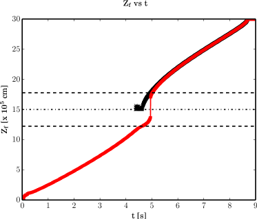
Figure 5: Horizontal position of the propagating front for simulation P3 (red) and E3 (black). Horizontal lines indicate the equator (dash dotted) and the belt as given by equation Eq. (23). For run P3, the crossing of the equator is clearly visible as the almost vertical transition around $t=5$ s. For run E3, the irregularities at the beginning correspond to the initial transient phase of flame ignition. The two simulations coincide to high degree, but the propagation from the equator to the south pole is not a mirror image of the propagation from the north pole to the equator.

Type	Run	$t_{1}$ [s]	$t_{2}$ [s]	$A$ [$10^{-2}$ s-3]	$B$ [$10^{-2}$ s-2]	$C$ [$10^{-1}$ s-1]	$D$ []	$\chi_{3}$	$\dot{\theta}_{0}$ [$10^{-1}$ s-1]	$I$ []	$\chi_{1}$
P–E	2	$0.50$	$2.04$	$-19.56$	$94.31$	$-9.05$	$0.32$	$0.36$	$4.73$	$-0.27$	$3.21$
P–E	3	$0.26$	$4.39$	$-0.42$	$2.26$	$1.82$	$0.06$	$0.51$	$2.03$	$0.07$	$1.02$
P–E	4	$0.22$	$6.09$	$-0.12$	$0.34$	$1.68$	$0.08$	$0.18$	$1.43$	$0.14$	$1.38$
P–E	5	$0.55$	$9.26$	$-0.09$	$1.21$	$0.42$	$0.11$	$0.29$	$0.89$	$0.07$	$1.51$
P–E	6	$0.37$	$6.30$	$-0.26$	$2.60$	$0.72$	$0.08$	$0.17$	$1.42$	$0.04$	$2.51$
P–E	7	$0.14$	$4.25$	$-0.03$	$-0.65$	$2.43$	$0.07$	$0.20$	$2.07$	$0.10$	$2.81$
E–P	2	$2.59$	$3.51$	$-56.51$	$506.48$	$-158.41$	$17.71$	$0.67$	$-7.85$	$2.87$	$1.32$
E–P	3	$4.96$	$8.70$	$-0.15$	$1.63$	$-2.59$	$2.04$	$0.77$	$-2.37$	$2.16$	$1.97$
E–P	4	$6.63$	$12.44$	$0.04$	$-2.09$	$1.12$	$1.04$	$0.32$	$-1.56$	$2.05$	$1.12$
E–P	5	$11.90$	$18.80$	$-0.06$	$2.24$	$-3.92$	$3.46$	$0.54$	$-1.24$	$2.45$	$2.14$
E–P	6	$7.44$	$12.50$	$-0.12$	$2.51$	$-3.24$	$2.48$	$0.25$	$-1.71$	$2.27$	$1.22$
E–P	7	$4.57$	$8.43$	$-0.33$	$5.72$	$-5.57$	$2.64$	$0.34$	$-2.37$	$2.06$	$0.85$

Table 2: Numerical parameters for the fits to the flame position during propagation. $A$, $B$ $C$ and $D$ should be used for Eq. (26), while $\dot{\theta}_{0}$ and $I$ apply to Eq. (25). The first values are for flames going from pole to equator (P-E), the second ones from equator to pole (E-P). The parameters of the simulations can be read in Table 1 with the corresponding number to those reported in the second column. Also reported are the $\chi$ values as from Eq. (27) for the cases of linear $\chi_{1}$ and cubic $\chi_{3}$ interpolation.

2.5 Flame on slowly rotating NSs

From previous studies, it was clear that the Coriolis force is important for flame propagation, but there exist cases, like IGR J17480-2446 spinning at $\nu=11$ Hz (see Altamirano et al., 2010; Cavecchi et al., 2011) where the rotation cannot provide confinement; nonetheless, they show pulsations during type I bursts. We therefore studied cases of low rotation.

We simulated a non rotating star, even though our initial conditions are not strictly speaking appropriate for this case, since there is no Coriolis force to confine the initial hot fluid. In this simulation the fluid spreads over the entire surface almost instantaneously and eventually burns, after $\sim 30$ s, in what is practically a 1D configuration. However, since most if not all NSs rotate we do not discuss this simulation any further.

We then considered a case with $\nu=10$ Hz, comparable to the frequency of IGR J17480-2446, for both polar and equatorial ignition. We found that, on one hand, after the fluid has oscillated a few times, simulation E1 ignites at $t\sim 4.5$ s. The temperature quickly exceeds $10^{9}$ K, starting the runaway, and the flame is visibly burning almost the whole domain, not being substantially confined (see Figure 6) similarly to the regimes of self-ignition. On the other hand, simulation P1, after a similar sloshing, has not yet ignited significantly after $t\sim 28$ s, but the temperature has been increasing at the pole, where $T\sim 10^{9}$ K, while most of the fluid is still cold. Since the temperature is increasing and fluid is burning at the pole, it is possible that at later times the burning could become significant, but we do not count this as a flame ignited at the initial ‘hot-spot’ and then propagated. Indeed, in the case of polar ignition the fluid that is hot at the pole is slowly heating the rest, but spreading over most of the surface. What we see confirms the fact that a sufficient amount of matter needs to be confined for ignition to happen. The difference in behaviour between simulation E1 and P1 is probably due to the difference in the extent of the two simulations.

3 Discussion and conclusions

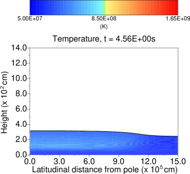
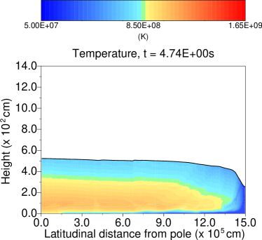
Figure 6: The late ignition of simulation E1 ($\nu=10$ Hz).

In Cavecchi et al. (2013), we showed the importance of the Coriolis force confinement for flame propagation considering only cases of spreading under constant Coriolis parameter. However, we did not consider meridional propagation, where Coriolis effect diminishes from pole to equator, and a question arose about whether the flame could cross the equator, where the confinement is absent. Moreover, we did not consider cases where the spin frequency was incapable of providing confinement at any latitude on the star. We analysed these problems in this paper.

First of all, we reported on our simulations that show how a flame ignited at one pole can successfully reach the equator and cross it to proceed to the other hemisphere, at least for $\nu\geq 10^{2}$ Hz. We also showed how thermal conductivity can affect the propagation and the general temperature profile over the surface. Finally, we showed that in our simulations there is a difference in the propagation of the flame from pole to equator and from equator to pole.

Equatorial crossing implies that the full star is probably burning during type I bursts, as is usually assumed. However, depending on the conductivity and the details of heat transport, one hemisphere may be significantly cooler than the other. For example, in the case of simulation P7 (Section 2.3 and Figure 3), where the conductivity is high enough, the highest temperature at the south pole is $\sim 1.6$ times the coolest one at the north pole, when propagation has finished. The thermal time scale in the vertical direction above the burning layer is, conservatively, $\lesssim 1$ s (Cumming & Bildsten, 2000; Weinberg et al., 2006), while in the horizontal direction it is longer by a factor approximately given by the square of the ratio of the length scales $(R_{\rm S}/H)^{2}\sim 10^{6}-10^{4}$, where $H$ is the thickness of the fluid above the burning layer and $R_{\rm S}$ is the star radius. Since the propagation takes up to few seconds, the difference in temperature at the bottom should be reflected in the emitting layers of the photosphere. This should be taken into account when analysing light curves which fit only one temperature. The temperature derived would be an average of the surface distribution and, for example, could affect conclusions about NS radius.

We found that the flame takes up to a few seconds to cross the equator, and, for realistic values of the opacity ($\kappa_{\rm{c}}\approx 0.07$ cm² g^-1, our fiducial value), the time needed decreases below 1s; of the order the time it takes to the flame to propagate downwards. This result has implications for all models and interpretations that have invoked any form of “stalling” of the flame at the equator. For example, the values we measure are too short compared to the times that Bhattacharyya & Strohmayer (2006) needed to explain double peak bursts, which are of the order of a few seconds. Those authors required the flame propagation to stop at the equator in order to explain bursts with double peaks: our simulations show that hydrodynamics alone does not allow for sufficient stalling. Of course, other mechanisms to stall the flame are still possible: in particular the role of magnetic field has to be considered carefully; as must the important case when the flame ignites at mid latitudes, so that there is not a single ring of fire propagating from pole to pole: this could imply that less burning fluid reaches the equatorial band, leading to a possible flume out. We plan to address this problem in a subsequent paper.

The asymmetry we found in the propagation from pole to equator as compared to from equator to pole, led us to provide a very basic fitting formula that could be used in order to simulate the propagation of a flame in a parametrized way, or at least provide a measure of the asymmetry between the two regimes. In particular, one can derive how much faster propagation from equator to pole is with respect to propagation from pole to equator. Note for example that the papers of Bhattacharyya & Strohmayer (2006) and, more recently, Chakraborty & Bhattacharyya (2014) assumed that the velocity of the flame depends only on the latitude and not also on the direction.

Finally, it is interesting to consider the simulations at frequency $\nu=10$ Hz. In such simulations the Coriolis force was not strong enough to confine the hot fluid. However, the fluid did eventually ignite, albeit on a much longer timescale and the flame and front were significantly different in nature with respect to the other, confined, cases: a great fraction of the fluid ignited almost simultaneously and only propagated through a small distance, similar to the regime of self ignition. The time needed for local ignition to finally happen probably depends on the interplay between the small confinement provided by the weak Coriolis force, the extent of the domain, as evidenced by the difference between the equatorial ignition and the polar ignition, the cooling prescription and the burning rate and energy release. However, one more conclusion can be drawn: our simulations support the arguments used by Cavecchi et al. (2011), who suggested that in the pulsar IGR J17480-2446 spinning at $11$ Hz, the presence of a hot-spot could not be achieved by the Coriolis force effects and therefore proposed that the surface asymmetries responsible for the strong measured pulsations might be caused by magnetic confinement.

Acknowledgements. We thank Frank Timmes for making his astrophysical routines publicly available. We also thank an anonymous referee for useful comments that improved this manuscript. YC and AW acknowledge support from an NWO Vrije Competitie grant ref. no. 614.001.201 (P.I. Watts). This paper benefitted from NASA’s Astrophysics Data System.

References

- Altamirano et al. (2010) Altamirano D., Watts A., Kalamkar M., Homan J., Yang Y. J., Casella P., Linares M., Patruno A., Armas Padilla M., Cavecchi Y., Degenaar N., Kaur R., van der Klis M., Rea N., Wijnands R., 2010, Astron. Telegram, 2932, 1
- Bhattacharyya & Strohmayer (2006) Bhattacharyya S., Strohmayer T. E., 2006, ApJ, 636, L121
- Bildsten (1995) Bildsten L., 1995, ApJ, 438, 852
- Braithwaite & Cavecchi (2012) Braithwaite J., Cavecchi Y., 2012, MNRAS, 427, 3265
- Cavecchi et al. (2011) Cavecchi Y., Patruno A., Haskell B., Watts A. L., Levin Y., Linares M., Altamirano D., Wijnands R., van der Klis M., 2011, ApJ, 740, L8
- Cavecchi et al. (2013) Cavecchi Y., Watts A. L., Braithwaite J., Levin Y., 2013, MNRAS, 434, 3526
- Chakraborty & Bhattacharyya (2014) Chakraborty M., Bhattacharyya S., 2014, ApJ, 792, 4
- Cumming & Bildsten (2000) Cumming A., Bildsten L., 2000, ApJ, 544, 453
- Fujimoto et al. (1981) Fujimoto M. Y., Hanawa T., Miyaji S., 1981, ApJ, 247, 267
- Galloway et al. (2010) Galloway D., in’t Zand J., Chenevez J., Keek L., Brandt S., 2010, in 38th COSPAR Scientific Assembly Vol. 38 of COSPAR Meeting, The Multi-INstrument Burst ARchive (MINBAR). p. 2445
- Güver et al. (2010) Güver T., Özel F., Cabrera-Lavers A., Wroblewski P., 2010, ApJ, 712, 964
- Kasahara (1974) Kasahara A., 1974, Mon. Weather Rev., 102, 509
- Lewin et al. (1993) Lewin W. H. G., van Paradijs J., Taam R. E., 1993, Space Sci. Rev., 62, 223
- Miller (2013) Miller M. C., 2013, preprint: 1312.0029
- Morsink et al. (2007) Morsink S. M., Leahy D. A., Cadeau C., Braga J., 2007, ApJ, 663, 1244
- Spitkovsky et al. (2002) Spitkovsky A., Levin Y., Ushomirsky G., 2002, ApJ, 566, 1018
- Steiner et al. (2010) Steiner A. W., Lattimer J. M., Brown E. F., 2010, ApJ, 722, 33
- Strohmayer & Bildsten (2006) Strohmayer T., Bildsten L., 2006,in Lewin W., van der Klis M., eds, Compact stellar X-ray sources, Cambridge Univ. Press, Cambridge, p. 113
- Suleimanov et al. (2011) Suleimanov V., Poutanen J., Revnivtsev M., Werner K., 2011, ApJ, 742, 122
- van der Toorn & Zimmerman (2008) van der Toorn R., Zimmerman J. T. F., 2008, Geophys. Astrophys. Fluid Dyn., 102, 349
- Weinberg et al. (2006) Weinberg N. N., Bildsten L., Schatz H., 2006, ApJ, 639, 1018
- White et al. (2005) White A. A., Hoskins B. J., Roulstone I., Staniforth A., 2005, Q. J. R. Meteorol. Soc., 131, 2081
- Zamfir et al. (2012) Zamfir M., Cumming A., Galloway D. K., 2012, ApJ, 749, 69