Fast and slow magnetic deflagration fronts in Type I X-ray bursts

Abstract

Type I X-ray bursts are produced by thermonuclear runaways that develop on accreting neutron stars. Once one location ignites, the flame propagates across the surface of the star. Flame propagation is fundamental in order to understand burst properties like rise time and burst oscillations. Previous work quantified the effects of rotation on the front, showing that the flame propagates as a deflagration and that the front strongly resembles a hurricane. However the effect of magnetic fields was not investigated, despite the fact that magnetic fields strong enough to have an effect on the propagating flame are expected to be present on many bursters. In this paper we show how the coupling between fluid layers introduced by an initially vertical magnetic field plays a decisive role in determining the character of the fronts that are responsible for the Type I bursts. In particular, on a star spinning at 450 Hz (typical among the bursters) we test seed magnetic fields of $10^{7}-10^{10}$ G and find that for the medium fields the magnetic stresses that develop during the burst can speed up the velocity of the burning front, bringing the simulated burst rise time close to the observed values. By contrast, in a magnetic slow rotator like IGR J17480–2446, spinning at $11$ Hz, a seed field $\gtrsim 10^{9}$ G is required to allow localized ignition and the magnetic field plays an integral role in generating the burst oscillations observed during the bursts.

1 Introduction

The Type I Bursts are X-ray flashes that last for tens to hundreds of seconds and are extremely bright, being able to produce up to $10^{38}$ erg/s. They are observed in approximately 100 sources, which are all low mass X-ray binaries where the accreting compact object is a neutron star (NS). The bursts are thermonuclear runaways that ignite in the accreted layers on the surface of the neutron stars (see Strohmayer & Bildsten, 2006; Galloway et al., 2008, for reviews). It is usually thought that ignition takes place at one position and then propagates across the surface (Shara, 1982). Thus, the observed lightcurve is the result of the convolution of the local emission evolution at every point on the surface and the propagation of the flame.

Type I burst provide a very promising means to extract information about the underlying NS, such as mass and radius that could put constraints on the equation of state of the matter in the core of the star (Strohmayer & Bildsten, 2006; Miller, 2013). However, many questions still remain open about the bursts, for example regarding what the most likely ignition site is, what nuclear reactions take place and how does the flame spreads over the surface. In order to disentangle the information we seek from the lightcurve, it is fundamental to understand how the flame propagates. The propagation mechanism is the focus of this paper.

Early discussion about possible mechanisms and the resulting flame velocity can be found in Wallace & Woosley (1981), Fryxell & Woosley (1982a), Fryxell & Woosley (1982b), Bildsten (1995) and Zingale et al. (2001) (see also Simonenko et al. 2012a, b). Spitkovsky et al. (2002) (from now on SLU02) suggested that localized ignition relies on confinement of the hot fluid. If not confined, the hot fluid would spread out over the surface, dissipate its heat and as a consequence no ignition would take place. In the presence of confinement, on the other hand, the heat would not dissipate and the flame would spread thanks to some heat transport mechanism at work between the hot and the cold fluid. Since most of the bursters spin faster than $\sim 100$ Hz, the authors suggested that the Coriolis force could provide the necessary confinement creating hurricane-like systems. The horizontal scale of both the ignition and the propagating front is that of a Rossby deformation radius, $R_{\rm{R}}=\sqrt{gH}/2\Omega$, where $g$ is the gravitational acceleration, $H$ the scale height of the fluid and $\Omega$ the angular velocity of the star. This was convincingly demonstrated by ab initio numerical simulations of Cavecchi et al. (2013, 2015). SLU02 also discussed the frictional coupling between the top and bottom layers and this is very important for this work (see below), but limited themselves to parametrizing its effect on the flame velocity. The simulations of Cavecchi et al. (2013, 2015) obtained propagation time scales in good agreement but generally somewhat longer than the observed rise times. Furthermore, they found that the principal mechanism responsible for the heat transport was the top-to-bottom conduction across the flame front. These simulations were performed without any magnetic field, which we show in this paper dramatically changes the velocity and the character of the flame.

Moreover, Cavecchi et al. (2011) discussed a very peculiar source, IGR J17480–2446 (from now on IGR J17480, see also Linares et al., 2011, Motta et al., 2011), which is spinning at approximately 11 Hz. This source is very important, since at 11 Hz the Coriolis force is not effective in confining the hot fluid, the Rossby radius being greater than the star’s radius. Nonetheless, IGR J17480 shows bursts and burst oscillations. The latter are fluctuations in the burst luminosity that are caused by an asymmetry in the emitting pattern modulated by the rotation of the star (first discovered by Strohmayer et al. 1996, they are seen in many bursters at different rotation rates, see Watts 2012 for a review). IGR J17480 is an accretion powered millisecond pulsar: fluctuations are also seen in the persistent emission, which implies that the accretion flow is channelled by a significant magnetic field (see Patruno & Watts, 2012, for a review on the behaviour of accretion powered X-ray pulsars). Finally, the burst oscillations and accretion powered oscillations of IGR J17480 are in phase. Based on this evidence, Cavecchi et al. (2011) proposed that the magnetic field could be the source of flame confinement in this case and estimated that a field $\gtrsim 10^{9}$ G was necessary.

In this paper we explore the effects of the magnetic field on the flame propagation of Type I Bursts in order to establish its interaction with the Coriolis force. We explore conditions that apply to the bursting X-ray pulsars, where the extra coupling between the layers provided by the magnetic field threading them is likely to affect the speed of flame propagation, increasing it and thus bringing our results to better agreement with the observations. We also dedicate a section specifically to the case of slow rotators like IGR J17480 where the magnetic field is needed to provide the extra confinement that the Coriolis force is not able to provide. In Section 2 we present the results of analytical calculation and the numerical simulations and in Section 3 we draw our conclusions.

2 The interaction between the magnetic field and the burning front

Here we will describe the results of our analytical calculations and numerical simulations, but first we summarize the numerical setup common to all runs.

2.1 Numerical setup

We use the code described in Braithwaite & Cavecchi (2012) and Cavecchi et al. (2013). An important assumption behind our simulations is hydrostatic equilibrium. This approach is particularly well suited for fluids whose horizontal stretch is much greater than the vertical extent, as in the case of the accreted layers of NSs. We use the so called $\sigma$ coordinate system (see Kasahara, 1974), a kind of pressure coordinate system. In the $\sigma$ coordinate system, the physical height of the fluid is fixed at the bottom to a constant value ($0$ cm in our case), while for every other grid point the physical height will change according to the fluid evolution. On the other hand, the pressure at the top is held constant throughout the simulation, while the bottom pressure will change according to the motion of the fluid. Of the various coordinate systems used in atmospheric physics, this is the logical choice in this context, as the computational domain can expand and contract to arbitrary degree in the vertical direction in response to the heating and cooling of the ocean.

The code uses finite differences and an explicit third-order low-storage Runge-Kutta scheme (Williamson, 1980) as the time stepper. The time step is limited by a Courant condition (see Braithwaite & Cavecchi, 2012). In our simulations the most limiting factors to the timestep are fluid motion and the magnetic field evolution. Spatial derivatives and integrals are fifth order accurate, while interpolations are sixth order (for details see Lele 1992 and Braithwaite & Cavecchi 2012). Variables are evaluated on a staggered grid: thermodynamic variables are defined at the centers of each grid cell, while velocities and magnetic field components are face centred. The staggered grid ensures good conservation of mass, energy, momentum and divergence of magnetic field (Braithwaite & Cavecchi, 2012, for the simulations in this paper, the average $\nabla B/{\rm{{B}}}_{0}$ is at maximum $10^{-12}$). The relation between density, pressure, temperature and composition is calculated with the routine helmeos of Timmes & Swesty (2000) where electrons can be arbitrarily degenerate and relativistic, ions are considered ideal gas and radiation pressure is also taken into account.

In this paper we use Cartesian coordinates, as in Cavecchi et al. (2013), but we set our coordinates system such that $x$ is pointing in the vertical direction, $z$ in the horizontal direction parallel to plane of the simulations (the direction of flame propagation) and $y$ is pointing out of the plane. We also neglect one horizontal direction, assuming symmetry along the $y$ direction. This configuration will help us elucidate most clearly the role of magnetic field in setting the fronts propagation speed. Vertically, our fluid is initially between $P_{\rm T}=10^{22}$ erg cm^-3 and $P_{\rm B}=e^{1.89}\times 10^{22}$ erg cm^-3, where $P_{\rm T}$ and $P_{\rm B}$ are the pressure at the top and at the bottom of the simulation. The value of 1.89 in the exponent for $P_{\rm B}$ implies that we are simulating approximately 1.89 scale heights. Horizontally, the domain is $6\times 10^{5}$ cm wide.

As in previous works, we set up an initial temperature profile which is meant to trigger the burst. It is independent of the vertical coordinate, but it has a horizontal dependence which is:

$$T=T_{0}+\frac{\delta T}{1+\exp[(z-z_{0})/\delta z]}$$ (1)

The parameters we use in this paper are $T_{0}=2\times 10^{8}$ K, $\delta T=2.81\times 10^{8}$ K, $z_{0}=9\times 10^{4}$ cm and $\delta z=3.6\times 10^{4}$ cm. $z_{0}$ corresponds to the position where the temperature is $T_{0}+\delta T/2$, while $\delta z$ is approximately the distance over which the temperature transitions from its maximum $T_{0}+\delta T$ to its minimum $T_{0}$.

We only consider helium burning via the triple-$\alpha$ reaction (Cumming & Bildsten, 2000)

$$Q_{\rm{n}}=5.3\times 10^{18}\rho_{5}^{2}\left(\frac{Y}{T_{9}}\right)^{3}e^{-4.4/T_{9}}\;\textrm{erg g${}^{-1}$ s${}^{-1}$},$$ (2)

and we simulate a fluid which is a mixture of helium and carbon.

We assume that the bottom boundary is not moving (no-slip condition). This is based on the consideration that the density of the burning layer becomes much smaller than the density of the ashes on which the layer rests. Therefore we allow for a buffer zone of pure carbon at the bottom of the simulation which is not affected by the flame propagation. In order to do so the initial composition is constant horizontally, but the helium fraction decreases downwards according to

$$Y=1-\frac{1}{1+\exp[-(\sigma-0.8)/1.6\times 10^{-2}]}$$ (3)

($\sigma=0$ at the top and $\sigma=1$ at the bottom). Erring on the side of caution, we also impose a damping force to prevent motion in the carbon layer near the boundary. Reassuringly, in later tests it turned out that switching off the damping force makes very little difference. We calculate the acceleration terms $\partial_{t}{U_{\rm z}}$ and $\partial_{t}{U_{\rm y}}$ and then multiply them by

$$\chi=\left\{\begin{array}[]{ccl}1&\sigma<0.82\\ \cos^{4}\left(\frac{\sigma-0.82}{0.1}\frac{\pi}{2}\right)&0.82<\sigma<0.92\\ 0&\sigma>0.92\end{array}\right.$$ (4)

The choice of this functional form for $\chi$ is made to ensure smoothness and the fact that the damping only acts within the buffer zone of carbon.

In our initial configuration the magnetic field is purely vertical and has a homogeneous value ${\rm{{B}}}_{0}$, which is different for different simulations. The gravitational acceleration is $g=2\times 10^{14}$ cm s^-2 and we use the plane-parallel approximation and a constant Coriolis parameter $f=2\Omega$ (the $f$-plane approximation). The fluid is initially at rest, with the horizontal velocities ${U_{\rm z}}={U_{\rm y}}=0$ cm s^-1. The physical conduction is calculated with an opacity fixed to $\kappa_{\rm{c}}=0.07$ cm² g^-1 (see details in Cavecchi et al., 2013).

On the horizontal components of the velocity we impose symmetric boundary conditions at the vertical boundaries and reflective conditions at the horizontal boundaries. For the horizontal components of the magnetic field we use antisymmetric boundary conditions both horizontally and vertically, while for the vertical component we use symmetric boundary conditions. By this choice, the field is forced to be perpendicular to the bottom and top surfaces. In all simulations presented here, we use horizontal and vertical resolutions of 192 and 90 grid points respectively. Our horizontal spatial resolution is therefore $3215$ cm, as in Cavecchi et al. (2013), which is greater than the scale height. This illustrates the suitability of the hydrostatic scheme. Our numerical hyperdiffusive scheme has viscosity parameters $\nu_{1}=0.03$ and $\nu_{2}=0.5$ (see Braithwaite & Cavecchi, 2012, for details). The corresponding values for the temperature and the helium fraction $Y$ numerical diffusivities are taken to be $1$ % of these. We also use an explicit hyperdiffusive scheme for the magnetic field to ensure stability and avoid zig-zags, it is calculated as a multiple of the one used for the velocity (Braithwaite & Cavecchi, 2012).

2.2 Analytical calculations

Run	${\rm{{B}}}_{0}\;(\textrm{G})$	$\nu\;(\textrm{Hz})$	$\tau_{\rm R}$ (s)	$\tau_{\rm fr}$ (s)	$R_{\rm{R}}$ (cm)	$v_{\rm f}$ (cm/s)	Strength
0	—	450	$1.77\times 10^{-4}$	—	$3.54\times 10^{4}$	$2.06\times 10^{5}$	—
1	$1\times 10^{7\phantom{0}}$	450	$1.77\times 10^{-4}$	$1.26\times 10^{-1}$	$7.91\times 10^{4}$	$7.28\times 10^{5}$	Weak
2	$1\times 10^{8\phantom{0}}$	450	$1.77\times 10^{-4}$	$1.26\times 10^{-3}$	$7.91\times 10^{4}$	$1.61\times 10^{6}$	Intermediate
3	$1\times 10^{9\phantom{0}}$	450	$1.77\times 10^{-4}$	$1.26\times 10^{-5}$	$7.91\times 10^{4}$	$4.78\times 10^{5}$	Intermediate-Strong
4	$1\times 10^{10}$	450	$1.77\times 10^{-4}$	$1.26\times 10^{-7}$	$7.91\times 10^{4}$	$1.29\times 10^{5}$	Strong
5	$1\times 10^{7\phantom{0}}$	011	$7.23\times 10^{-3}$	$1.26\times 10^{-1}$	$3.24\times 10^{6}$	—	Weak
6	$1\times 10^{8\phantom{0}}$	011	$7.23\times 10^{-3}$	$1.26\times 10^{-3}$	$3.24\times 10^{6}$	—	Intermediate - Strong
7	$1\times 10^{9\phantom{0}}$	011	$7.23\times 10^{-3}$	$1.26\times 10^{-5}$	$3.24\times 10^{6}$	$4.59\times 10^{5}$	Strong
8	$1\times 10^{10}$	011	$7.23\times 10^{-3}$	$1.26\times 10^{-7}$	$3.24\times 10^{6}$	$1.33\times 10^{5}$	Strong

Table 1: Values of the initial purely vertical magnetic field ${\rm{{B}}}_{0}$, the spin frequency $\nu=\Omega/2\pi$, the rotational $\tau_{\rm R}=1/f$ and effective frictional (magnetic) timescales Eq. (14) defined in Section 2.2, the Rossby radius $R_{\rm{R}}=\sqrt{gH}\tau_{\rm R}$ and the flame spread velocity $v_{\rm f}$ for the main runs discussed in the text. The last column reports the rough classification used in Section 2.3. The estimates for $\tau_{\rm fr}$ are obtained substituting the value of ${\rm{{B}}}_{0}$ in Eq. (16), using $\tau_{\rm burn}=0.1$ s and setting the numerical constants to $1$. For $R_{\rm{R}}$ we use $g=2\times 10^{14}$ cm s^-2 and $H=10^{3}$ cm. $v_{\rm f}$ is the value given by a linear fit to the horizontal position of maximum burning as a function of time.

As shown in (Cavecchi et al., 2013), when the flame propagates in the absence of a magnetic field, the burning front is located along an inclined but nearly horizontal surface that separates as yet unburnt fuel from actively burning material (see e.g. Figure 1, left panel). A strong vertical shear is set up within the front. In an atmosphere without friction the horizontal velocity is in (quasi) geostrophic balance with the horizontal pressure gradient. As a consequence, the vertical shear of the velocity is given by the thermal wind relation (a hurricane-like structure, see Pedlosky 1987 and SLU02 and Figure 1 right panel):

$${\partial v_{y}\over\partial x}={g\over f}{\partial\log\rho\over\partial z}$$ (5)

As the horizontal gradient of the density is concentrated within the burning front, so is the vertical shear of the horizontal fluid velocity. When a magnetic field is present, this shear directly couples to the pre-existing vertical magnetic field $B_{x}={\rm{{B}}}_{0}$ and generates the horizontal field $B_{y}$ via ${\rm{d}}B_{y}/{\rm{d}}t=B_{x}\partial v_{y}/\partial x$; here $d/dt$ is the Lagrangian derivative for the fluid element coming through the front.

The horizontal field generates magnetic stress that back-reacts on the shear flow. The result is that the geostrophic balance is (partially) broken, which can lead to faster penetration of the hot burning fluid in the top layers of the unburnt fuel. The acceleration of the front propagation due to the mechanical top-bottom momentum exchange was noted in SLU02 who introduced a phenomenological timescale $\tau_{\rm fr}$ for the frictional coupling and showed that the front velocity reaches maximum when $\tau_{\rm fr}\sim 1/f$. Here we study the effect of the back-reaction of the flow-generated magnetic field and show that it does indeed accelerate the front propagation for a certain range of magnetic field strengths (compare to sections 2.3 and 3.7 of SLU02).

Let $\vec{v}_{\rm h}$ be the horizontal velocity at the top side of the burning front. The vertical shear is, to order of magnitude, $v_{h}/h$ where $h$ is the vertical width of the front. The horizontal magnetic field generated in a fluid element upon its passage through the front is

$$\vec{B}_{\rm h}\sim B_{x}{\tau_{\rm n}\vec{v}_{\rm h}\over h}.$$ (6)

Here $\tau_{\rm n}$ is the nuclear burning time which is also the characteristic time for a fluid element to cross the front. The horizontal magnetic field causes horizontal acceleration of the top velocity of the burnt-fuel

$$\vec{a}_{\rm mag}\sim-{B_{x}\vec{B}_{\rm h}\over 4\pi\rho H},$$ (7)

where $\rho$ and $H$ are the density and scale height of the burning fluid (Heng & Spitkovsky, 2009). The overall horizontal acceleration of the burning fluid is caused by three physically distinct force fields: the horizontal pressure gradient, the Coriolis force, and the magnetic back-reaction force:

$$\vec{a}_{h}=\alpha_{1}g{H\over L}\vec{e}_{z}-\vec{f}\times\vec{v}_{h}-\alpha_{2}{{\rm{{B}}}_{0}^{2}\over 4\pi\rho H}{\tau_{\rm n}\over h}\vec{v}_{h},$$ (8)

where $\alpha_{1}$ and $\alpha_{2}$ are numerical coefficients of order $1$, $L$ is the horizontal extent of the front surface and we used ${{B}_{\rm x}}={\rm{{B}}}_{0}$, the seed field. To complete this equation, we note that first,

$$\vec{a}_{h}\sim\alpha_{0}\vec{v}_{h}/\tau_{\rm burn},$$ (9)

and secondly,

$$L\sim\tau_{\rm burn}\vec{v}_{h}\cdot\vec{e}_{z}.$$ (10)

Here $\tau_{\rm burn}\sim\tau_{\rm n}H/h$ is the timescale for the front to burn vertically through a patch of the ocean and $\alpha_{0}$ is a constant of order $1$. Eq. (9) reflects the fact that the fluid has time $\tau_{\rm burn}/\alpha_{0}$ to accelerate from zero to $\vec{v}_{h}$ as the front burns vertically through the ocean, while Eq. (10) reflects the fact that it is the velocity component $\vec{v}_{h}\cdot\vec{e}_{z}$ that is responsible for the hot fluid covering the unburnt cold fluid.

Eqs. (8), (9) and (10) form a closed system that can be solved for the two horizontal components of velocity $\vec{v}_{h}\cdot\vec{e}_{z}$ and $\vec{v}_{h}\cdot\vec{e}_{y}$. The $z$-component is representative of the horizontal velocity of the burning front (compare SLU02, equation 34); it is given by

$$v_{\rm f}\sim\vec{v}_{h}\cdot\vec{e}_{z}=\left[{{\alpha_{1}gH\over\tau_{\rm burn}}\frac{1/\tau}{f^{2}+1/\tau^{2}}}\right]^{1/2}.$$ (11)

Here

$$\tau=\left(\alpha_{2}{\tau_{\rm burn}\over\tau_{\rm A}^{2}}+\frac{\alpha_{0}}{\tau_{\rm burn}}\right)^{-1},$$ (12)

where

$$\tau_{\rm A}=H/v_{\rm A}={\sqrt{4\pi\rho}H/{\rm{{B}}}_{0}}$$ (13)

is the Alfvén crossing timescale and $v_{\rm A}={\rm{{B}}}_{0}/2\sqrt{\pi\rho}$ the Alfvén speed. It can be seen that the effective frictional time is given in our case by

$$\tau_{\rm fr}=\frac{\tau_{\rm A}^{2}}{\alpha_{2}\tau_{\rm burn}}$$ (14)

Let us consider several limits of this equation. In the non-magnetic limit, so that $\tau_{\rm A}\gg\tau_{\rm burn}$, the front velocity becomes (using $1/f\ll\tau_{\rm burn}$)

$$v_{\rm f}\sim\sqrt{\alpha_{1}\alpha_{0}}{\sqrt{gH}\over f\tau_{\rm burn}},$$ (15)

in agreement with Cavecchi et al. (2013) and SLU02. Note that $v_{\rm f}$ is independent of the magnetic field coupling. However, for higher magnetic fields

$$\tau_{\rm A}=0.01\left({H\over 10^{3}\hbox{ cm}}\right)\left({\rho\over 10^{5}\hbox{ g}/\hbox{cm}^{3}}\right)^{1/2}\left({{\rm{{B}}}_{0}\over 10^{8}\hbox{ G}}\right)^{-1}\hbox{s}$$ (16)

may well be much smaller than $\tau_{\rm burn}\sim\hbox{few}\times 0.1\hbox{s}$ so that $\tau\sim\tau_{\rm fr}$. So the next relevant comparison is that of the timescale $\tau_{\rm fr}$ with $\tau_{\rm R}=1/f$. In the strong-field case where $\tau_{\rm fr}\ll\tau_{\rm R}$, which corresponds to

$${\rm{{B}}}_{0}\gg\bar{{\rm{{B}}}_{0}} = 2.5\times 10^{8}\left({H\over 10^{3}\hbox{ cm}}\right)\left({\rho\over 10^{5}\hbox{ g}/\hbox{cm}^{3}}\right)^{1/2}\times$$ (17)

$$\left({\nu\over 400\hbox{ Hz}}\right)^{1/2}\left({\alpha_{2}\tau_{\rm burn}\over 0.1\hbox{ s}}\right)^{-1/2}\hbox{G},$$

the speed of the front becomes independent of the rotation rate:

$$v_{\rm f}\sim\sqrt{gH}\sqrt{\frac{\alpha_{1}\tau_{\rm fr}}{\tau_{\rm burn}}}\sim\sqrt{gH}\frac{\tau_{\rm A}}{\tau_{\rm burn}}\sqrt{\frac{\alpha_{1}}{\alpha_{0}}}.$$ (18)

Finally, in the intermediate regime of ${\rm{{B}}}_{0}\sim\bar{{\rm{{B}}}_{0}}$, i.e. $\tau_{\rm fr}\sim\tau_{\rm R}(\ll\tau_{\rm burn})$ the magnetic field strongly accelerates the speed of the flame propagation, reaching the maximum at ${\rm{{B}}}_{0}=\bar{{\rm{{B}}}_{0}}$:

$$\hbox{max}\left(v_{\rm f}\right)=\sqrt{\alpha_{1}/2}{\sqrt{gH}\over\sqrt{f\tau_{\rm burn}}}.$$ (19)

The analytic arguments of this section are confirmed by the direct numerical simulations described below.

2.3 Numerical simulations

We simulated different configurations varying the initial vertical magnetic field intensity and the spin frequency of the star. We consider ${\rm{{B}}}_{0}$ in the range $10^{7}-10^{10}$ G (broadly covering the range of magnetic fields in accretion powered X-ray pulsars Mukherjee et al. 2015) and $\nu=450$ Hz and $\nu=11$ Hz; a summary of the parameters for each run is reported in Table 1. We divide our simulations into three rough categories, which we call strong, intermediate and weak magnetic field based on the $\tau_{\rm R}/\tau_{\rm fr}$ ratio and the development of the hurricane structure. We discuss these cases separately, comparing them to the case of Run 0, which has no magnetic field present and is rotating at $\nu=450$ Hz. This simulation evolves as those discussed in Cavecchi et al. (2013). In particular, it has a well defined hurricane structure identifiable by the thermal wind (see Figure 1, right panel). It also has a well defined burning region without turbulence (Figure 1, left panel).

2.3.1 Strong magnetic field ($10^{10}$ G)

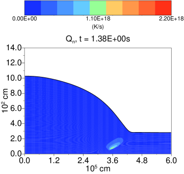
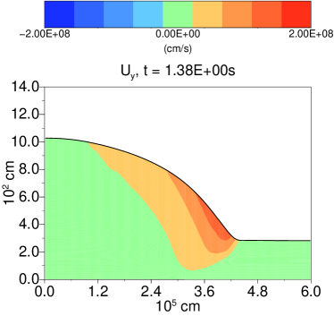
Figure 1: Burning rate (left) and velocity in the y direction (perpendicular to the plane of the simulation - right) for the the non magnetic case, Run 0, with $\nu=450$ Hz. The flame along the hot-cold fluid interface without turbulence and the thermal wind are clearly visible.

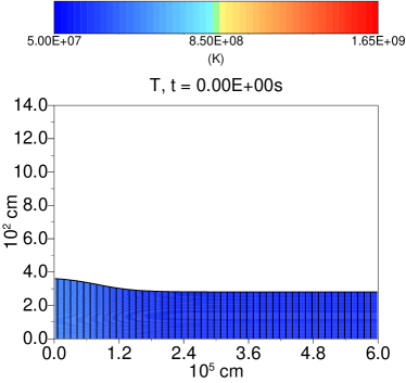
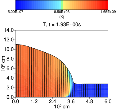
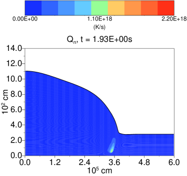
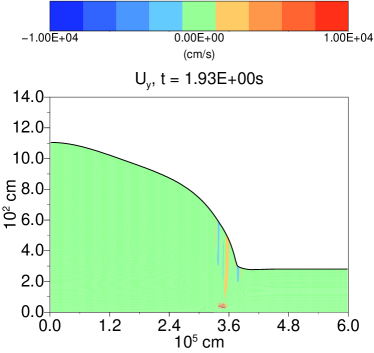
Figure 2: Upper panels: initial and late conditions of the propagating flame in the case of Run 4, ${\rm{{B}}}_{0}=10^{10}$ G and $\nu=450$ Hz. The magnetic field lines are superimposed on the temperature profile. The magnetic field is strong enough to prevent most of the fluid motion. Even when the flame is propagating, the magnetic field lines are barely bent. Lower panels: nuclear reaction rate (left) and velocity in the y direction (right) for the same simulation. The absence of ${U_{\rm y}}$ shows that the propagation is driven by the sole magnetic confinement, since the Coriolis force is almost completely suppressed, to the point that a different color scale is needed to highlight the small components of the velocity.

We start with the case of ${\rm{{B}}}_{0}=10^{10}$ G , Run 4. This field strength is at the upper end of the estimated burster magnetic field distribution. In this case the initial overpressure at the top of the temperature perturbation cannot bend the magnetic field lines significantly. Indeed, the frictional time scale is much faster than the rotational period (see Table 1). The initial motion is quickly suppressed and with no significant z velocity, no significant Coriolis force appears that can generate the thermal wind.

In Figure 2 we show the results for Run 4. The top left panel shows the initial configuration of the magnetic field superimposed on the temperature profile. This configuration is the same for all simulations, apart from the value of the seed magnetic field ${\rm{{B}}}_{0}$. On the right, we show the system at a later time: it can be seen that the field lines have not been bent significantly. The maximum bending is at the interface between hot and cold fluid, barely visible at $z\sim 3.6\times 10^{5}$ cm. We observed the trace particle sliding down the hot-cold interface when the flame is approaching. When the flame has passed, they move mostly vertically along the straightened back field lines. Eventually, they only follow the expansion of the fluid, not moving anymore with respect to the fluid itself.

We can compare this simulation to Run 0 (same spin, $\nu=450$ Hz, but without magnetic field) looking at the lower panels of Figure 2 and at Figure 1. The first significant feature is that no hurricane structure has developed, as can be seen by the absence of any strong velocity ${U_{\rm y}}$ perpendicular to the plane in Figure 2. Accordingly, the field has been bent in the y direction only slightly (${{B}_{\rm y}}/{{B}_{\rm x}}\sim 0.1$ at its maximum). The only exception is a weak component of ${U_{\rm y}}$ right above the flame, where a component of at maximum $1.5\times 10^{5}$ cm s^-1 is seen briefly oscillating back and forth. We can see also a very weak component of the velocity at the top of the front, this is associated with the Coriolis force reaction to the motion of the fluid at the top of the interface. The second feature is that after a steady state propagation has been established, the structure of the flame is very similar to the purely Coriolis confined one, even if the interface between hot and cold fluid is steeper, in the sense that there is no turbulence at the front, as opposed to what we see in the other simulations (see below). If we compare the estimated values for $\tau_{\rm R}$ and $\tau_{\rm fr}$ from Table 1 in the case of Run 4, we can see that the magnetic coupling should strongly dominate over the Coriolis force and therefore the length scale for the confinement should also be smaller than the Rossby radius.

In Cavecchi et al. (2013) we discussed how the propagation speed scales proportional to $\propto R_{\rm{R}}/H$, since $R_{\rm{R}}$ and $H$ set the inclination of the interface along which conduction can take place and the shallower the interface (longer $R_{\rm{R}}$) the more effective conduction is. In the general case, $R_{\rm{R}}$ should be replaced by the hot-cold fluid interface horizontal length scale, be it imposed by the Coriolis force or the magnetic field or a combination of the two forces. As a confirmation, we find that the flame speed in the present case is slower than in the case without magnetic field since the flame is confined over a shorter distance. This simulation corresponds to the case of strong friction discussed in Section 2.2. The overpressure on the left is acting on all the layers of fluid ahead, due to strong magnetic vertical coupling, and the velocity is predominantly in the z direction, i.e. the horizontal direction of flame propagation in our notation.

2.3.2 Weak magnetic field ($10^{7}$ G)

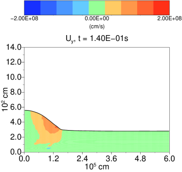
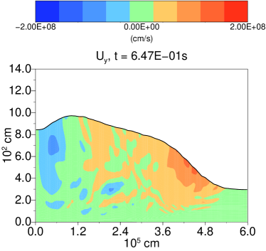
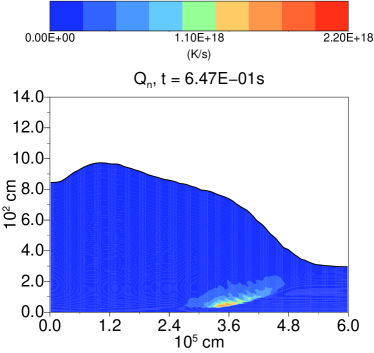
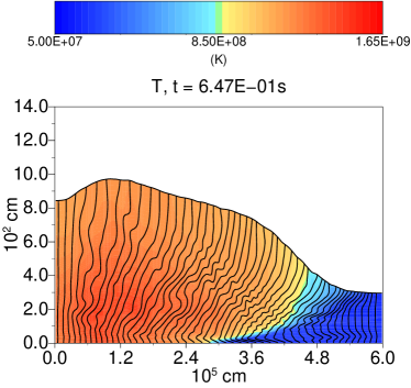
Figure 3: Results for Run 1, ${\rm{{B}}}_{0}=10^{7}$ G and $\nu=450$ Hz. Upper panel: velocity perpendicular to the plane ${U_{\rm y}}$ at an early (left) and later (right) stage. Initially the height peak described in the text is not present: it develops at $\sim 0.3$ s, when the flame has passed the peak horizontal position. Lower panel: burning rate (left) and temperature profile (right) in the steady state propagation regime. Field lines are overplotted on the temperature profile.

We move now to the other extreme of ${\rm{{B}}}_{0}=10^{7}$ G , Run 1. This approximately corresponds to the lower end of the magnetic field distribution for bursters. This case is much more dynamical. As can be seen in Figure 3 the late evolution of the flame and the field is strongly influenced by the motion of the fluid. Despite the fact that we call this case weak, it has to be borne in mind that even here the magnetic field is playing a role in the dynamics.

At the beginning, the magnetic field is not capable of confining the initial pressure imbalance of the fluid and the fluid spills over sideways. At $\nu=450$ Hz, the Coriolis force is strong enough to intervene and a hurricane structure begins to develop (Figure 3, upper left panel). The fluid motion drags the magnetic field along and strong horizontal components are generated. This agrees well with the fact that $\tau_{\rm R}\ll\tau_{\rm fr}$ (see Table 1). However, the flame is very different from Run 0 (the case without magnetic field) as can be seen comparing the lower left panel of Figure 3 to Figure 1. In the case with weak magnetic field, we can see that the hot-cold fluid interface is much more extended. As a consequence, when we measure the propagation speed, we find that in the case of ${\rm{{B}}}_{0}=10^{7}$ G the flame moves faster than in the case of no magnetic field. Note that the value reported in Table 1 is the result of a linear fit to the horizontal position of maximum burning as a function of time. In this particular case, we found that the position of the flame was better fitted by a parabola than a line. This means that the velocity was accelerating till the flame reached the boundary. The value we report is therefore an average value.

The reason for the longer interface and the higher speed is the reaction of the magnetic field which partly obstructs the Coriolis force. For example, it can be seen that the y component of the velocity, which characterizes the hurricane structure and ensures the Coriolis confinement, is smaller in absolute value than in the case with no magnetic field and is also limited to layers far above the level where most of the burning takes place. The magnetic field component ${{B}_{\rm y}}$ is maximum at the flame location and steadily decreases (apart from superimposed oscillations induced by waves, see below) once the flame has passed. The reduced confinement is responsible for the longer extent of the interface. This situation is analogous to the case when friction is beginning to be significant, but it is still weaker than the Coriolis force. When the flame reaches the right boundary, the helium fraction is higher than in the case of no rotation or strong magnetic field. This can be easily understood if we consider that given the higher propagation speed, the hot fluid burnt for less time.

Finally, we note that after the initial flame has developed, oscillations set in along the hot-cold fluid interface, near the flame. Here the baroclinicity is highest and Alfvén waves are excited and move along the magnetic field lines. The waves propagate also backwards, at the base of the field lines. These, in turn, excite other waves along the field lines behind the flame, leading to the intricate configuration shown in the right, lower panel of Figure 3.

There is an additional difference when comparing this case with the one of strong magnetic field or with the one of pure rotation: after $\sim 0.3$ s a peak forms in the height of the fluid (see Figure 3, upper right panel and lower panels). The position of the peak ($z\sim 1.0\times 10^{5}$ cm) does not seem to change appreciably for the rest of our simulation, and it is close to the position where our initial temperature perturbation was half of its maximum value ($z\sim z_{0}$ in Eq. 1). At this position the field lines are bent and remain bent for the rest of the simulation. When the flame reaches the boundary on the right, the fluid is still burning and eventually the peak disappears.

In order to confirm the correspondence with the initial perturbation, we ran a further simulation where the initial temperature distribution was given by Eq. (1), but with $z_{0}=1.5\times 10^{5}$ cm. We verified that also in this case a peak develops and it is now at $z\sim 1.5\times 10^{5}$ cm, i.e. where the centre of the new perturbation is. In both cases the magnetic field keeps memory of the initial perturbation. The damping factor described in Section 2.1 is not the origin of the peak, since simulations with higher vertical resolution, the same physical parameters, but without the damping showed the same behaviour. The peak was there and even more pronounced. Inspection of the temperature distribution shows that the base of the fluid, below the peak, has a higher temperature (see Figure 3, lower right panel). It appears that the heat is deposited in this region, mainly by viscous heating, following the waves that are localized below the peak. Our viscosity is mostly artificial and this may produce excessive heating, but if a similar heating process were proven to be physical, then such a peak could be the origin of an asymmetry in the emission during the burst rise and therefore lead to burst oscillations.

2.3.3 Intermediate strength magnetic field ($10^{8}$ - $10^{9}$ G)

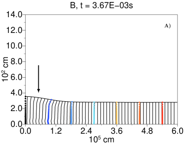
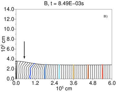
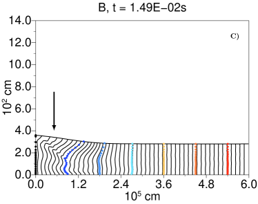
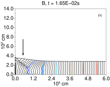
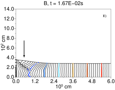
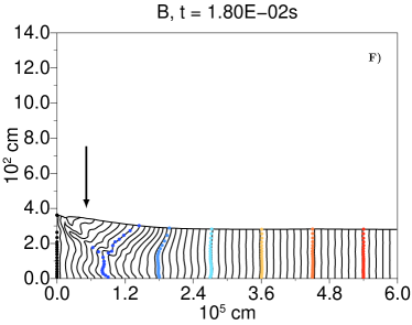
Figure 4: Run 2, $\nu=450$ Hz and ${\rm{{B}}}_{0}=10^{8}$ G . The initial evolution of the thermal structure on the left added at $t=0$ s to ignite the fluid. Shown are the magnetic field lines and tracer particles. The color of the particles is related to their initial horizontal position. The hot fluid that is trying to spill over is eventually blocked and directed downwards resulting in an early dilution of the original heat reservoir. The arrows indicate the horizontal position of the perturbation described in the text.

Finally, we address the case of intermediate strength magnetic field. The behaviour of Run 2, ${\rm{{B}}}_{0}=10^{8}$ G , is again different from the previous ones. In this case the initial heat reservoir perturbation that we impose on the temperature to trigger the burst is partly diluted during the very early stages of the simulation. The whole flame propagation is very chaotic.

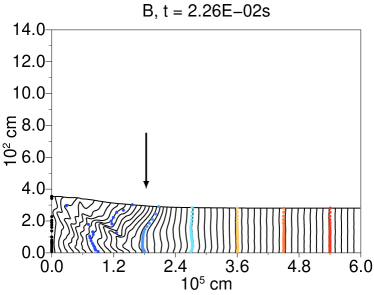
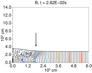
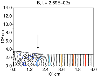
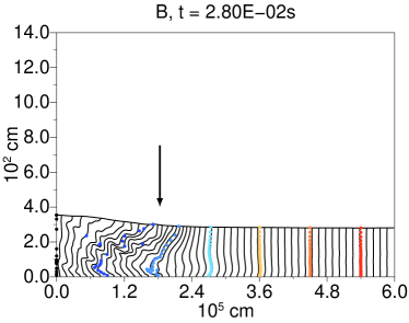
Figure 5: Continuation of the early evolution of Run 2 from Figure 4, ${\rm{{B}}}_{0}=10^{8}$ G $\nu=450$ Hz. Shown are the magnetic field lines with tracer particles superimposed. The arrows indicate the horizontal position of the later evolution of the perturbation described in the text.

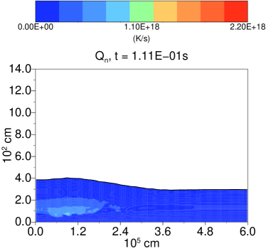
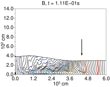
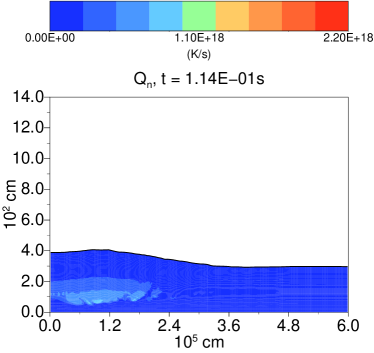
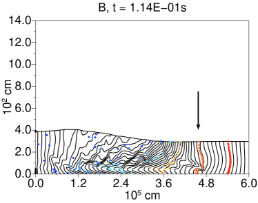
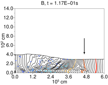
Figure 7: Continuation of the early evolution of Run 2 from Figure 6, ${\rm{{B}}}_{0}=10^{8}$ G $\nu=450$ Hz. Shown are the burning rate (left) and the magnetic field lines (right), with tracer particles superimposed. The arrows indicate the horizontal position of the perturbation described in the text at later time.

The partial dilution of the initial heat reservoir perturbation occurs in the following fashion. As can be seen in Figure 4, the hot fluid in the upper left corner of the simulation begins to slide to the right (panels A and B). The field lines follow the fluid, bending near the top at an approximate height of $\sim 2\times 10^{2}-3\times 10^{2}$ cm. Then, the curvature of the knee of the bent field lines increases and secondary, alternating, knees form below (panels B and C). The configuration becomes unstable around the upper knee (panel D) with the hot and cold fluid mixing: the field lines reconnect and the hot fluid moves right- and downwards, while the cold fluid goes up- and leftwards. This triggers a cascade of fluid rolls that propagate right- and downwards (panels D, E and F). Analogously, later in the simulation, we see a similar perturbation affecting the field lines. The perturbation propagates like a wave triggered where the weight of the fluid that is moving near the top of the simulation bends the field lines and these form a knee. The wave propagates from the formation of the knee down- and rightwards across the field lines: see the configuration of the field line around $z\sim 1.8\times 10^{5}$ cm in Figure 5 or the field line just after $z\sim 2.4\times 10^{5}$ cm at $t\sim 3.89\times 10^{-2}$ s in Figure 6. This perturbation propagates towards the right of the simulation (see for example the field lines around $z\sim 4.8\times 10^{5}$ cm in the second column of Figure 7), while additional waves are excited along the field lines that have been already hit by the front of the perturbation. Note that at $t\sim 1.11\times 10^{-1}$ s another front of perturbation is now reaching $z\sim 4.8\times 10^{5}$ cm (Figure 7), at $t\sim 1.3\times 10^{-1}$ s it will be at $z\sim 5.4\times 10^{5}$ cm and it will reach the right boundary at $t\sim 1.4\times 10^{-1}$ s. In order to find in which range of magnetic field strength the same initial bending of the field lines that leads to the beginning of the perturbation takes place, we ran a few more simulations and found that the same phenomenon is seen down to ${\rm{{B}}}_{0}\sim 3\times 10^{7}$ G, but not anymore at ${\rm{{B}}}_{0}\sim 5\times 10^{8}$ G. Note that this range encompasses the critical value $\bar{{\rm{{B}}}_{0}}$ of Eq. (17).

The partial dilution of the heat reservoir did not cause the flame to die, and the burning began right at the start of the simulation, but the flame is different from the well confined flame of the other cases we have treated so far. A pseudo steady state propagation is established: from the main burning region, hot fluid tongues are launched up- and rightwards, these eventually turn downwards and leftwards when they reach regions where magnetic field lines have been compressed together. Secondary flames keep igniting where the front of the perturbation brings hotter fluid to regions of higher density. The new flame will propagate backwards till it joins the main burning region. First examples of these secondary burning blobs can be seen in Figure 6. Clearer examples can be seen in Figure 7, since the burning is by now more intense also in the new flames, where the association of the secondary ignition sites with compressed field lines is more clear. The fluid keeps rolling between regions where the field lines have been compressed, mixing hot and cold fluid. An example can be spotted noting the deformed shape of the field lines between $z\sim 2.4\times 10^{5}$ cm and $z\sim 3.0\times 10^{5}$ cm at $t\sim 1.17\times 10^{-1}$ s in the lowest right panel of Figure 7 or in the right, top panel of Figure 8 between $z\sim 4.2\times 10^{5}$ cm and $z\sim 4.8\times 10^{5}$ cm.

These rolling eddies appear where the fluid is more baroclinic and driven by the baroclinic version of buoyancy. In this sense they are a form of convection (Pedlosky, 1987). The fluid follows the compressed field lines on its left when going upwards, and the motion that follows after the fluid is stopped by the denser field lines ahead is reminiscent of the behaviour of the Parker instability (Parker, 1966). This is understandable when considering the configuration of the field lines in this simulation. The field has been stretched and has developed a strong horizontal component. When the fluid at the top is stopped, it rests on these stretched lines, which are naturally subject to the instability. The fluid slides down and backwards along the inclination of the lines. When it stops, this fluid has higher entropy than the fluid above it and consequently is pushed vertically upwards again, generating the rolling motion between the regions of denser field lines. The continuous ignition of the fluid repeats this process until the right boundary is reached and the cycle cannot proceed anymore.

The flame proceeds forward very fast, $v_{\rm f}\sim 1.6\times 10^{6}$ cm s^-1, in this fashion, until by $t\sim 3\times 10^{-1}$ s it reaches the boundary, where the field lines are being compressed. Finally, the fluid temperature reaches $T\sim 10^{9}$ K everywhere and by $t\sim 5.98\times 10^{-1}$ s the fluid is expanding vertically approximately homogeneously and the field lines are straightening up. We note that these propagation timescales are in very good agreement with the observed rise times of observed bursts.

Given the very fast initial phase where the flame reaches the extent of the boundary while the temperature does not rise above $10^{9}$ K, most of the fluid is still unburnt and it will be burned during the subsequent homogeneous expansion of the whole layer. Comparing with the case of no magnetic field (Run 0) we find that during the whole propagation the hurricane structure is present, but the perpendicular velocity ${U_{\rm y}}$ is of smaller amplitude, (the maximum absolute amplitude is roughly half the one of the case with ${\rm{{B}}}_{0}=10^{7}$ G , Run 1, or of rotation only, Run 0). This is again in agreement with the fact that the flame velocity for Run 2 is faster than for Runs 0 and 1. The smaller the perpendicular velocity, the smaller the Coriolis force and the greater the propagation speed. In the left panel of Figure 9 we show the profile of the perpendicular velocity ${U_{\rm y}}$, where the thermal wind is perturbed by the reaction of the Coriolis force to the horizontal $z$ motion of the rolling eddies and the Alfvén waves excited along the field lines. Finally we note that during the flame propagation after $t\sim 8.46\times 10^{-2}$ s (Figure 6) there is a temperature (and height) peak that is moving with the flame. The thermal wind is positive (out of the plane) at the flame front and negative (into the plane) behind. This propagation would appear as an expanding ring on the surface of the neutron star, at least until the effects of curvature become important. This is different from what we saw in the case of weak magnetic field, since there the peak was remaining at the same horizontal position, while the burning region expands, but also this configuration may lead to burst oscillations during the burst rise.

We also ran a simulation with ${\rm{{B}}}_{0}=10^{9}$ G (Run 3, see Figure 8 lower panels). Despite the fact that the simulation with ${\rm{{B}}}_{0}=10^{8}$ G is much more chaotic than this one and that no dilution of the initial heat reservoir takes place when ${\rm{{B}}}_{0}=10^{9}$ G , these two cases share some similarities. The steady state configuration of Run 3 has a burning region which is more homogeneous than the one of Run 2, but still it shows secondary burning bubbles and rolling eddies at the front (visible at $3.6\times 10^{5}\rm{cm}\lesssim z\lesssim 4.2\times 10^{5}\rm{cm}$ in the lower panels of Figure 8). This simulation bears similarities also with the case of strong field, since the spilling of the fluid is more controlled than in the cases of lower magnetic field. However, the front is much more elongated than in that case, and flame propagation is consequently faster. The flame is faster also than in the case of no magnetic field, Run 0, but slower than in the case of ${\rm{{B}}}_{0}=10^{7}$ G , Run 1, and ${\rm{{B}}}_{0}=10^{8}$ G , Run 2. The perpendicular velocity ${U_{\rm y}}$ is even smaller than in the case of ${\rm{{B}}}_{0}=10^{8}$ G (Run 2), which is to be expected since the magnetic stress back-reaction increases with the seed magnetic field intensity. Moreover, the ${U_{\rm y}}$ velocity field at the front is oscillating and no real thermal wind is present (right panel of Figure 9). This is again very similar to what we see in the case of strong field, so that the case of ${\rm{{B}}}_{0}=10^{9}$ G should be regarded as a transition between the intermediate and strong field regimes. This behaviour is consistent with the fact that in this case $\tau_{\rm fr}<\tau_{\rm R}$ (Table 1) which implies that at this point the magnetic coupling has become stronger than the Coriolis force.

Run 2, ${\rm{{B}}}_{0}=10^{8}$ G , is the configuration that yields the fastest propagation speed among our configurations. This corresponds to a situation where the frictional coupling is most effective in increasing the speed of the flame and the speed value is near its peak. Indeed, ${\rm{{B}}}_{0}=10^{8}$ G is very close to our estimate of the critical field $\bar{\rm{{B}}}_{0}$. SLU02 discussed how in this case the flame propagates so fast that the ignition would be almost horizontally uniform: that is indeed what we observe. Increasing the field strength even more increases the coupling further, and the flame velocity will begin to decrease. The speed is expected to decrease because the pressure imbalance at the top has to push both the top and lower layers that are strongly coupled by the magnetic field. This is what we see happening in the case of Run 3, ${\rm{{B}}}_{0}=10^{9}$ G and more drastically in the case of Run 4, ${\rm{{B}}}_{0}=10^{10}$ G .

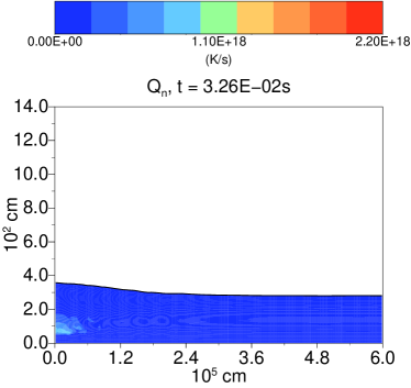
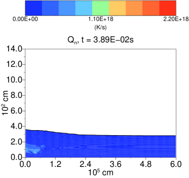
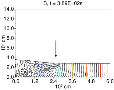
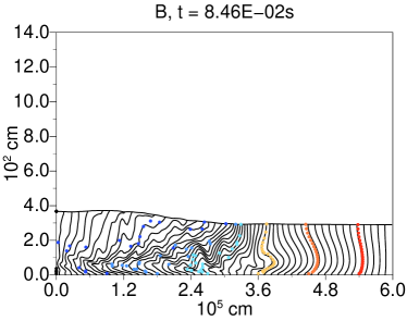
Figure 6: Continuation of the early evolution of Run 2 from Figure 5, ${\rm{{B}}}_{0}=10^{8}$ G $\nu=450$ Hz. Shown are the burning rate (left) and the magnetic field lines (right), with tracer particles superimposed. The arrow indicates the horizontal position of the perturbation described in the text at later time.

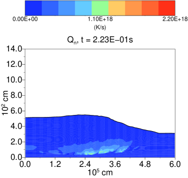
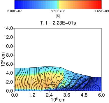
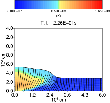
Figure 8: The burning rate (left) and the temperature profile (right), with magnetic field lines superimposed of the later stages of the flame propagation for Run 2, ${\rm{{B}}}_{0}=10^{8}$ G $\nu=450$ Hz, (upper panels) and Run 3, ${\rm{{B}}}_{0}=10^{9}$ G $\nu=450$ Hz (lower panels).

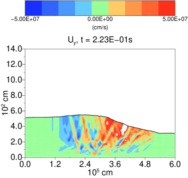
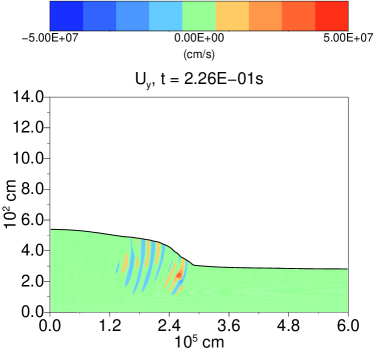
Figure 9: The profile of the perpendicular velocity ${U_{\rm y}}$ in the case of ${\rm{{B}}}_{0}=10^{8}$ G (Run 2, left) and ${\rm{{B}}}_{0}=10^{9}$ G (Run 3, right) and $\nu=450$ Hz. In the first case the thermal wind structure is still present, however disturbed by the reaction of the Coriolis force to the rolling eddy motions and by the Alfvén waves along the field lines, while in the second case no hurricane has developed. Note that the color scale is different from the ones of Figures 1, 2 and 3. The white color patches correspond to velocity values above $5\times 10^{7}$ cm s^-1.

2.3.4 Slow rotation - the case of IGR J17480

Here we discuss the special case of a star spinning at $\nu=11$ Hz, the rotation rate of the source IGR J17480 discussed in Cavecchi et al. (2011). Recall that in this case the Coriolis force is not capable of confining the fluid. We ran simulations using the same fields as we used for the case $\nu=450$ Hz, so that comparison will be easier, but the concept of weak, intermediate and strong field should now be revisited: apart from the case with ${\rm{{B}}}_{0}=10^{7}$ G , all fields have frictional time scales smaller than the rotational period and should be regarded as strong.

First, we ran another simulation, Run 8, with a seed magnetic field of ${\rm{{B}}}_{0}=10^{10}$ G , as in the case of Run 4. As expected, the acceleration due to magnetic stresses dominates that due to the Coriolis force therefore controlling the flame propagation and the simulation results are almost indistinguishable from those at higher spin (Run 4). Therefore, also in this case, the flame propagation resembles that confined only by the Coriolis force at higher frequency (see Section 2.3.1) and thus we expect that a slow rotating source in this regime of magnetic field will still have a phenomenology similar to faster rotators without magnetic field. A simulation with ${\rm{{B}}}_{0}=10^{9}$ G , Run 7, also shows a behaviour very comparable to the case with the same field strength and $\nu=450$ Hz, Run 3. That, again, can be understood in terms of the frictional time scale (see Table 1). Furthermore, we noticed that the thermal wind structure was absent at $\nu=450$ Hz, a fact that showed how the Coriolis force was no longer playing a significant role for the confinement and propagation.

When the field is ${\rm{{B}}}_{0}=10^{8}$ G , Run 6, some differences between fast and slow rotation become more noticeable. After an initial phase where the fluid strongly bends the field lines, weak burning develops at the left end of the simulation, which triggers rolls that propagate towards the right similar to those of Run 2 (${\rm{{B}}}_{0}=10^{8}$ G , $\nu=450$ Hz). These rolling eddies compress the fluid lines and climb over them at intervals. We see also fluid flowing down- and leftwards along the fluid lines when the eddies hit a new region of compressed lines. This propagation is similar to the case with ${\rm{{B}}}_{0}=10^{8}$ G and $\nu=450$ Hz; however, at low rotation the length scale of these eddies is obviously longer (Figure 10, upper panels). This velocity of propagation is very fast and at $t\sim 2.6\times 10^{-1}$ s, the whole layer is horizontally approximately homogeneously burning. It is difficult to track a neatly defined flame front, since secondary ignition sites ignite continuously due to the rolling eddies. Therefore, we do not report any velocity in Table 1, but a rough estimate gave $v_{\rm f}\sim 3.5\times 10^{6}$ cm s^-1. Finally, when the burning is roughly homogeneous we see a convective pattern with three or four cells above the most intensely burning layer. These rolls disappear gradually during the rise of the burst, leaving at the end only two rolls, one per side, which eventually disappear as well, before the peak of the burst (Figure 10, lower panels).

Finally, in the case of ${\rm{{B}}}_{0}=10^{7}$ G , Run 5, we see that the fluid sloshes back and forth many times before ignition, which takes place at $t\sim 1.94$ s. This is to be expected, since neither the Coriolis force nor the field (which is weaker) can significantly confine the fluid within the simulation domain and the waves bounce back only because of the reflecting boundaries. Without the magnetic field the fluid behaved very similarly, starting ignition at around $t\sim 1.77$ s. Convection develops above the horizontal layer that is burning, similarly to the case with ${\rm{{B}}}_{0}=10^{8}$ G and $\nu=11$ Hz. Note that such late ignitions are probably caused by the finiteness of our simulation domain and the 2D dimensionality which prevents any dissipation in the $y$ direction, while a neutron star spherical surface is much wider and in reality the flame would probably flume out. We conclude that the results of our simulations for the case of $\nu=11$ Hz are in agreement with the predictions of Cavecchi et al. (2011): a field of ${\rm{{B}}}_{0}\gtrsim 10^{9}$ G is required in order to have flame confinement and propagation.

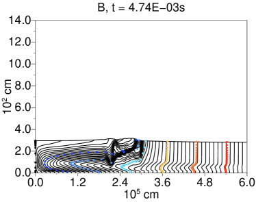
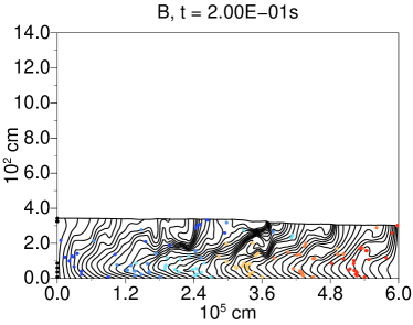
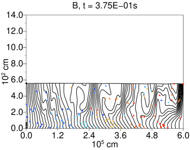
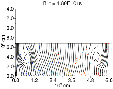
Figure 10: The evolution of Run 6, ${\rm{{B}}}_{0}=10^{8}$ G $\nu=11$ Hz, at different stages. Shown are magnetic field lines with tracer particles superimposed. Particles with the same color had the same horizontal position at the beginning of the simulation. Upper panels: the fluid is confined by the magnetic field only (left). A very fast initial propagation takes the form of rolling eddies (right). Lower panels: later stages of the burst when ignition is almost horizontally homogeneous. Convection sets in (left) and eventually subsides (right).

3 Summary and conclusions

3.1 Summary of simulations at fast rotation ($\nu=450$ Hz)

In this paper we have presented 2D simulations of Type I bursts in the presence of both rotation and an initially vertical magnetic field. We have shown that in the case of a magnetic field of ${\rm{{B}}}_{0}=10^{10}$ G , what we called the strong magnetic field case, flame propagation is independent of the rotation rates we used ($\nu=11$ Hz, $\nu=450$ Hz). The magnetic field prevents the development of any thermal wind (the hurricane structure described in SLU02 and Cavecchi et al. 2013) by inhibiting significant horizontal motions. The flame structure resembles very closely the one of a fast rotator in the sense that the fluid is not affected by turbulence, but propagation is slower. On the other hand, we found that in the presence of a weak magnetic field (${\rm{{B}}}_{0}=10^{7}$ G ), the fluid confinement depends on the Coriolis force. In the case of fast rotation the presence of the field affects the structure of the front, making it more extended in the horizontal direction. This has the net effect of speeding up the flame propagation compared to a case with rotation only.

A striking feature we found in the case of fast rotation with ${\rm{{B}}}_{0}=10^{7}$ G is the development of a peak in the fluid height, due to high temperature, at a location approximately coincidental with the size of our initial heat reservoir in the temperature profile. A test with different size of the perturbation confirmed that the position of the peak is related to the initial conditions. From our simulations it looks like the origin of higher temperature is due to extra heating (mainly viscous) deposited by waves localized below the peak. Our viscosity is numerical, but if a similar mechanism were at work in nature, this would imply that there exist cases where a weak magnetic field (when compared to the Coriolis force, in the sense defined in Section 2.3) would lead to the presence of an asymmetry in the emission pattern during the rise of the burst. This, in turn, could lead to the presence of burst oscillations. We also found that the velocity of the flame seemed to be accelerating until it reached the right boundary. Indeed, the flame propagation was better fitted by a parabola than a straight line. It would be interesting to check whether a constant velocity would ever be reached and on what length scale. In particular, it would be interesting to follow the evolution of this case on the spherical surface of a NS.

The case of intermediate strength magnetic field with ${\rm{{B}}}_{0}=10^{8}$ G at fast rotation showed a very remarkable series of results. First, we saw a temperature and height peak propagating with the flame, which would look like an expanding ring on the surface of the neutron star, until the effects of curvature would become significant. The duration and the possible effects on burst oscillations of this ring should be tested in 3D simulations. Secondly, we saw a perturbation triggered by the bending of the field lines at the very beginning of the simulation. However, this did not prevent ignition and flame propagation. Finally, this configuration showed that rolling eddies form at the flame front, which mix the hot and cold fluid and speed up the flame propagation by even an order of magnitude when compared to the case without magnetic field. Also, similar eddies at the flame front form in the case of a field ${\rm{{B}}}_{0}=10^{9}$ G . In this case, however, there is no trace of the thermal wind and the hurricane structure that we still observe when ${\rm{{B}}}_{0}=10^{8}$ G and ${\rm{{B}}}_{0}=10^{7}$ G . The burst proceeds with speed higher than in the case without magnetic field.

The presence of the eddies at the flame front is very interesting, since they provide a means of heat conduction over a long length scale helping in speeding up flame propagation as compared to when only conduction is taking place (see for example the discussion of Fryxell & Woosley, 1982b, about the different speeds in the case of conduction, convection and turbulence). These giant rolls could also be responsible for bringing burning ashes to higher layers in the atmosphere, a fact that could lead to the generation of absorption lines (Weinberg et al., 2006). Their behaviour, in relation with rotation rate and magnetic field strength, is very close to what is expected for convective rolls in the standard Bénard problem with both rotation and magnetic field (Chandrasekhar, 1961). Indeed, their size decreases with increasing magnetic field (in our cases, going from ${\rm{{B}}}_{0}=10^{8}$ G to ${\rm{{B}}}_{0}=10^{9}$ G , for example) and increases with decreasing rotation frequency (as clearly seen for the case with ${\rm{{B}}}_{0}=10^{8}$ G going from $\nu=450$ Hz to $\nu=11$ Hz). However, during the bursts we do not have a standard Bénard configuration, since the fluid can be in motion due to the thermal wind structure (as in the case of ${\rm{{B}}}_{0}=10^{8}$ G ), the flame front is continuously moving and so is the source of heat that sets the temperature gradient. Furthermore, the configuration at the front is affected by the baroclinic motions, by the compression of the cold fluid under the weight of the expanding hot fluid and the Parker instability. The rolls clearly have an important role that could be amplified in 3D and further study is required.

3.2 Summary of simulations at slow rotation ($\nu=11$ Hz) and implications for the source IGR J17480

We performed simulations of a star with $\nu=11$ Hz and magnetic fields in the same range as for the fast rotator case: $10^{7}\leq{\rm{{B}}}_{0}\leq 10^{10}$ . Simulations with ${\rm{{B}}}_{0}=10^{10}$ G and ${\rm{{B}}}_{0}=10^{9}$ G behaved practically identically to the cases with $\nu=450$ Hz, since the magnetic field was providing most of the confining force also in the case of fast rotation. The case with ${\rm{{B}}}_{0}=10^{8}$ G showed similar eddies to the analogue case at faster rotation, even though the length scale of the eddies was longer. The initial phase of flame propagation was even faster and eventually the explosion of the burst was mostly homogeneously horizontal. In the case with ${\rm{{B}}}_{0}=10^{7}$ G neither the magnetic tension nor the Coriolis force was strong enough to provide any confinement and this led to the dispersion of the initial heat reservoir over the full horizontal extent of the simulations. We still saw a very delayed ignition, but we think that this is due to the smallness of our simulation domain compared to the size of the neutron star surface, a fact which prevents a more realistic dissipation.

We note that our simulations for the case of $\nu=11$ Hz confirm the conclusions of Cavecchi et al. (2011) about the case of IGR J17480. This source was discovered in 2010 in the globular cluster Terzan 5 (Bordas et al., 2010). It was found that IGR J17480 displayed both accretion powered oscillations and burst oscillations at $\nu=11$ Hz (Strohmayer & Markwardt, 2010; Altamirano et al., 2010; Papitto et al., 2011). The accretion powered and the burst oscillations had highly accurately matching phases and frequencies (Cavecchi et al., 2011). This matching and the slow rotation rate led the authors to exclude the possibility that the Coriolis force could confine the flame and they also concluded that neither a Coriolis force confined hot-spot nor global modes could explain the burst oscillations. Based on approximated analytic calculations the authors estimated that the magnetic field of IGR J17480 could provide a dynamically effective confining force for the flame if $B\gtrsim 10^{9}$ G.

Therefore, a field weaker than ${\rm{{B}}}_{0}=10^{8}$ G would not confine the fluid and both ignition and burst oscillations should not be expected. At ${\rm{{B}}}_{0}=10^{8}$ G , confinement is still weak and even if we do see the explosion leading to a burst, we do not expect to see any burst oscillation at this regime, since the flame propagates very fast and the whole domain ignites almost coincidentally. On the other hand, a field of ${\rm{{B}}}_{0}=10^{9}$ G or higher shows a confined propagating flame, and we conclude that this is the minimum field intensity needed to have bursts that could display burst oscillations.

3.3 Discussion of numerical and nuclear burning effects

Before tackling the effects of the magnetic field, we will briefly discuss possible contributions that may affect the flame velocity we measure.

One possible factor is resolution-related numerical effects. We could not perform full convergence tests for the simulations with magnetic field since that would have consumed many months, an amount of computational resources that we do not have at the moment. However, the convergence tests in Cavecchi et al. (2013) showed that our code at similar resolutions to those used in this paper is converging, even if somewhat slowly. Furthermore, short convergence tests for the initial stages of runs $0-4$ showed the following trends.

Run 0, being purely hydrodynamical, behaves exactly as the tests performed in Cavecchi et al. (2013) with the velocity of the flame decreasing slowly with resolution; run 4 behaves similarly, but the velocity at this stages seems already almost converged (velocity changed by only $\sim 5$ %). In the case of run 1 we note that at resolutions much lower than those in the text, many of the waves associated with the flame would not be resolved. The velocity measured at this very initial stages is increasing with resolution, by $\sim 30$ %, but the velocity we report in the text is evaluated at later stages that we did not reach in this short convergence tests. Runs 2 and 3, on the other hand, should be more sensitive to resolution. This is linked to the fact that (a) the maximum flame position is difficult to track for both simulations and (b) the convective rolls are captured differently at different resolutions. This situation is complicated by the fact that at different resolution our numerical diffusivities are different (Cavecchi et al., 2013). As expected, run 2 is more affected by resolution from the beginning, but the qualitative behaviour is the same as in our reference run, with the development of the initial perturbation described in Section 2.3.3. The velocity in run 3 seems almost converged in the early stages (difference in velocity is $\sim 0.01$ %), but we cannot exclude that it might change at later stages due to the onset of rolls (see Section 2.3.3).

Other important factors are the physical burning and the opacity. Timmes (2000) performed a detailed analysis of 1D horizontal laminar propagation of the flames, studying its dependence on the reaction network, thermodynamic conditions and conductivity. Timmes’ simulations were in good agreement with order of magnitude calculations predicting a velocity of the flame $\propto\sqrt{Q/\kappa}$, with $Q$ the burning rate and $\kappa$ the opacity. A direct comparison to his results is impossible, mainly because the flame in our simulations, being vertically resolved, crosses different levels of pressure, while Timmes’ simulations were performed at constant pressure. Furthermore, we include cooling and fluid dynamics, which are absent in that analysis. In Cavecchi et al. (2013) we proved that flame propagation in type I bursts can be expressed as a vertical flame velocity $v_{\rm f\perp}$ times a geometrical boosting factor set by the slope of the hot-cold fluid interface: $v_{\rm f}\sim v_{\rm f\perp}R_{\rm Ro}/H$. As we showed in the present paper, in many cases the net effect of the magnetic field is to interfere with the Coriolis force, therefore changing the slope of the interface and the boosting factor. Since this is the focus of the paper, we discuss it in the next section. However, a different conduction or a different burning regime as used by Timmes will change the vertical flame speed $v_{\rm f\perp}$. Our conduction is constant across the whole domain. While this is an approximation, it is less important than the reaction rate, since the value we use is calibrated to be the expected opacity at the conditions near the most burning regions. On the other hand, our reaction rate is limited to helium burning into carbon. A more extended reaction network with quick energetic reactions will boost the propagation speed by increasing the energy production rate at the vertical flame front. That is because of the flame speed dependence $v_{\rm f\perp}\propto\sqrt{Q}$ (Timmes, 2000). Slow reactions, like for example those limited by $\beta$-decays in hydrogen rich material, will probably have a smaller impact as long as there are faster ones occurring, since the slow ones will take place in the wake of the vertical flame front. Direct numerical simulations are needed to better quantify these effects in the complex dynamical configurations of the type I bursts, in order to quantify the effects of composition and nuclear burning on the propagation speed and surface temperature distribution during all the stages of the bursts. This will also have a direct impact on the prediction and measurement of burst oscillations.

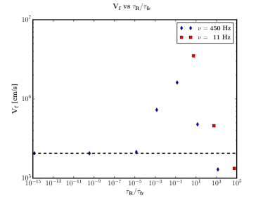
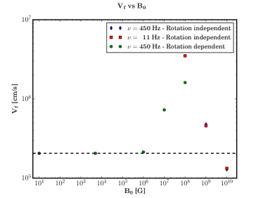
Figure 11: Left: velocity of the flame versus $\tau_{\rm R}/\tau_{\rm fr}$. The blue diamonds represent the results for the fast rotator $\nu=450$ Hz, while the red squares are the results for the slow rotator case ($\nu=11$ Hz). The horizontal dashed line indicates the velocity of the flame when magnetic field is absent. Right: velocity of the flame versus ${\rm{{B}}}_{0}$ (note that ${\rm{{B}}}_{0}\propto 1/\tau_{\rm A}\propto 1/\sqrt{\tau_{\rm fr}}$). The blue diamonds represent the results for the fast rotator $\nu=450$ Hz and the red squares are the results for the slow rotator ($\nu=11$ Hz) when $\tau_{\rm R}\gg\tau_{\rm fr}$ and the flame velocity is independent of rotation. The green circles are the results for the fast rotator when $\tau_{\rm R}<\tau_{\rm fr}$ and the velocity is affected by the Coriolis force. In these plots we include results both from Table 1 and footnote 8.

3.4 The effect of the magnetic coupling on flame propagation speed

The most remarkable result of our simulations is about the effect that the magnetic field has on the propagation speed of the flame. We summarize the results regarding the flame speed $v_{\rm f}$ in Figure 11. Note that we include the values both from Table 1 and footnote 8 (compare also to figure 2 of SLU02).

In Section 2.2 we argued that there exists a field strength at which the propagation speed is maximal (Eq. 17, ${\rm{{B}}}_{0}\sim 2.8\times 10^{8}$ G for $\nu=450$ Hz). We also discussed how for decreasing field strength less effective coupling will lead to lower values of the flame speed, to the point that when $\tau_{\rm R}\ll\tau_{\rm fr}$ the velocity should be independent of the magnetic field (Eq. 15). This is the trend we see in the left panel of Figure 11 looking at the results for $\nu=450$ Hz (blue diamonds). If ${\rm{{B}}}_{0}\gg\bar{{\rm{{B}}}_{0}}$, $\tau_{\rm R}\gg\tau_{\rm fr}$, the flame speed is expected to decrease continuously with the field strength. Again, this can be verified in Figure 11.

We also noted that when $\tau_{\rm R}\gg\tau_{\rm fr}$ the velocity of propagation should depend only on the field strength via the frictional time scale $\tau_{\rm fr}$ (Eq. 18). This is more clearly seen in the right panel of Figure 11. There, the blue diamonds ($\nu=450$ Hz) and the red squares ($\nu=11$ Hz) represents the results obtained in this regime. In particular, it can be seen that the velocities for ${\rm{{B}}}_{0}=10^{9}$ G and ${\rm{{B}}}_{0}=10^{10}$ G overlap almost perfectly. In contrast, for ${\rm{{B}}}_{0}\leq 10^{8}$ G the results at $\nu=450$ Hz deviate from those at $\nu=11$ Hz because of the increasing importance of the Coriolis force on the formers (green circles), as expected.

We conclude that our simulations confirm our analysis on the importance of the magnetic field in regulating the flame speed by providing an effective frictional coupling among the fluid layers and we note that for realistic field strengths we obtain speed values that are already in very good agreement with the velocities inferred from observations.

Acknowledgements. We thank Frank Timmes for making his astrophysical routines publicly available. Y.C. and A.W. acknowledge support from an NWO Vrije Competitie grant ref. no. 614.001.201 (PI: Watts). This work was also sponsored by NWO Exacte Wetenschappen (Netherlands Organization for Scientific Research, Physical Sciences) for the use of supercomputer facilities, with financial support grant no. SH-337-15 (PI: Cavecchi). The paper benefitted from NASA’s Astrophysics Data System.

References

- Altamirano et al. (2010) Altamirano D., et al., 2010, The Astronomer’s Telegram, 2932, 1
- Bildsten (1995) Bildsten L., 1995, ApJ, 438, 852
- Bordas et al. (2010) Bordas P., et al., 2010, The Astronomer’s Telegram, 2919, 1
- Braithwaite & Cavecchi (2012) Braithwaite J., Cavecchi Y., 2012, MNRAS, 427, 3265
- Cavecchi et al. (2011) Cavecchi Y., et al., 2011, ApJ, 740, L8+
- Cavecchi et al. (2013) Cavecchi Y., Watts A. L., Braithwaite J., Levin Y., 2013, MNRAS, 434, 3526
- Cavecchi et al. (2015) Cavecchi Y., Watts A. L., Levin Y., Braithwaite J., 2015, MNRAS, 448, 445
- Chandrasekhar (1961) Chandrasekhar S., 1961, Hydrodynamic and hydromagnetic stability
- Cumming & Bildsten (2000) Cumming A., Bildsten L., 2000, ApJ, 544, 453
- Fryxell & Woosley (1982a) Fryxell B. A., Woosley S. E., 1982a, ApJ, 258, 733
- Fryxell & Woosley (1982b) Fryxell B. A., Woosley S. E., 1982b, ApJ, 261, 332
- Fushiki & Lamb (1987) Fushiki I., Lamb D. Q., 1987, ApJ, 317, 368
- Galloway et al. (2008) Galloway D. K., Muno M. P., Hartman J. M., Psaltis D., Chakrabarty D., 2008, ApJS, 179, 360
- Heng & Spitkovsky (2009) Heng K., Spitkovsky A., 2009, ApJ, 703, 1819
- Kasahara (1974) Kasahara A., 1974, Monthly Weather Review, 102, 509
- Lele (1992) Lele S. K., 1992, Journal of Computational Physics, 103, 16
- Linares et al. (2011) Linares M., Chakrabarty D., van der Klis M., 2011, ApJ, 733, L17+
- Miller (2013) Miller M. C., 2013, preprint (arXiv:1312.0029)
- Motta et al. (2011) Motta S., et al., 2011, MNRAS, 414, 1508
- Mukherjee et al. (2015) Mukherjee D., Bult P., van der Klis M., Bhattacharya D., 2015, MNRAS, 452, 3994
- Papitto et al. (2011) Papitto A., D’Aì A., Motta S., Riggio A., Burderi L., di Salvo T., Belloni T., Iaria R., 2011, A&A, 526, L3+
- Parker (1966) Parker E. N., 1966, ApJ, 145, 811
- Patruno & Watts (2012) Patruno A., Watts A. L., 2012, preprint (arXiv:1206.2727)
- Pedlosky (1987) Pedlosky J., 1987, Geophysical Fluid Dynamics. Springer-Verlag
- Shara (1982) Shara M. M., 1982, ApJ, 261, 649
- Simonenko et al. (2012a) Simonenko V. A., Gryaznykh D. A., Litvinenko I. A., Lykov V. A., Shushlebin A. N., 2012a, Astronomy Letters, 38, 231
- Simonenko et al. (2012b) Simonenko V. A., Gryaznykh D. A., Litvinenko I. A., Lykov V. A., Shushlebin A. N., 2012b, Astronomy Letters, 38, 305
- Spitkovsky et al. (2002) Spitkovsky A., Levin Y., Ushomirsky G., 2002, ApJ, 566, 1018
- Strohmayer & Bildsten (2006) Strohmayer T., Bildsten L., 2006, New views of thermonuclear bursts. Cambridge University Press, pp 113–156
- Strohmayer & Markwardt (2010) Strohmayer T. E., Markwardt C. B., 2010, The Astronomer’s Telegram, 2929, 1
- Strohmayer et al. (1996) Strohmayer T. E., Zhang W., Swank J. H., Smale A., Titarchuk L., Day C., Lee U., 1996, ApJ, 469, L9+
- Timmes (2000) Timmes F. X., 2000, ApJ, 528, 913
- Timmes & Swesty (2000) Timmes F. X., Swesty F. D., 2000, ApJS, 126, 501
- Wallace & Woosley (1981) Wallace R. K., Woosley S. E., 1981, ApJS, 45, 389
- Watts (2012) Watts A. L., 2012, ARA&A, 50, 609
- Weinberg et al. (2006) Weinberg N. N., Bildsten L., Schatz H., 2006, ApJ, 639, 1018
- Williamson (1980) Williamson J. H., 1980, Journal of Computational Physics, 35, 48
- Zingale et al. (2001) Zingale M., et al., 2001, ApJS, 133, 195