Reconstructing heavy Higgs boson masses in Type X Two-Higgs Doublet Model with a light pseudoscalar

Abstract

We analyze the prospects of reconstructing the mass of a heavy charged Higgs boson in the context of a Type X two-Higgs doublet model where a light pseudoscalar $A$ in the mass range $40-60$ GeV is phenomenologically allowed, and is in fact favoured if one wants to explain the muon anomalous magnetic moment. The associated production of charged Higgs with the pseudoscalar $A$ and subsequent decay of the charged Higgs into a $W$ and $A$, is found to be our relevant channel. The branching ratio for $H^{+}\to W^{+}A$ with $M_{H^{+}}\sim 200$ GeV, is close to 50%. The hadronic decay of the $W$ boson, coupled with the leptonic decays of $A$ into a tau and muon pair, help in identifying the charged Higgs. The neutral heavy Higgs, being degenerate with the charged Higgs for most of the allowed parameter space of the model, also contributes to similar final states. Thus both of these particles are reconstructed within a band of about 10 GeV.

1 Introduction

In describing new physics an extended scalar sector can be of relevance in several contexts including supersymmetry, CP-violation and dark matter. Of the possible scenarios, two-Higgs doublet models (2HDMs) stand out as minimalistic but phenomenologically rich options, whose signatures can be tested at colliders. There are four broad categories of 2HDMs which respect natural flavor conservation at the tree level, due to the presence of some discrete symmetry in the Lagrangian. These are usually named Type I, Type II, Type X (or lepton specific) and Type Y (or flipped) Gunion et al. (2000); Djouadi (2008); Branco et al. (2012). This paper focuses on identifying the collider signatures of the heavy Higgs bosons in Type X 2HDM, which has a viable region of parameter space that explains the muon $g-2$ discrepancy Brown et al. (2001); Bennett et al. (2006). This region allows for a sufficiently light ($40-60$ GeV) pseudoscalar, coupled with a high value of tan $\beta$, that can give enhanced (positive) two-loop contribution to the anomalous muon magnetic moment Cheung et al. (2001); Cheung and Kong (2003); Jegerlehner and Nyffeler (2009); Broggio et al. (2014); Chun et al. (2015). Such low values of $M_{A}$, the pseudocalar mass, are consistent with all experimental limits Kanemura et al. (2014a); Broggio et al. (2014); Chun et al. (2015).

In this scenario, one scalar doublet has Yukawa couplings with quarks only, while the other one couples to leptons alone. This results in the “hadrophobic” nature of the couplings of the heavy Higgs bosons and the pseudoscalar, allowing a light pseudoscalar to escape detection at LHC. It has been demonstrated Broggio et al. (2014); Chun et al. (2015); Chun and Kim (2016) that the neutral pseudoscalar $A$ in type X 2HDM can be as light at 40-60 GeV or even lighter in certain regions in the parameter space respecting all the constraints coming from collider data, muon $g-2$, flavor constraints, electroweak precision data and theoretical constraints from vacuum stability and perturbativity. There have been several studies exploring signatures of the scalar sector of the type X 2HDM at LHC and $e^{+}e^{-}$ colliders Su and Thomas (2009); Kanemura et al. (2012); Kanemura et al. (2014b, a); Chun et al. (2015). In a recent work, the issue of reconstructing such a light pseudocalar was studied Chun et al. (2017), utilizing the decay mode of the pseudoscalar into a muon pair, enabling reconstruction of the sharp invariant mass peak.

For large $\tan\beta$, the light pseudoscalar with mass around 50 GeV has a $\tau^{+}\tau^{-}$ branching ratio close to unity, and a $\mu^{+}\mu^{-}$ branching ratio of the order of $0.35\%$. We consider the channel $p~{}p\to H^{\pm}A$, where the charged Higgs decays via $H^{\pm}\to W^{\pm}A$ and then the pseudoscalar $A$’s decay to a tau or muon pair, i.e. $A\to\mu^{+}\mu^{-}$ and $A\to\tau^{+}\tau^{-}$. The invariant mass reconstruction from the muon pair will clearly be able to identify the pseudoscalar with a sharp resonance. We show how one can reconstruct the charged Higgs ($H^{\pm}$) and the heavier neutral scalar ($H$), making use of the $A$-reconstruction strategy delineated in Chun et al. (2017).

In Section 2 we recapitulate the Type X 2HDM and point out how the parameter space of the model gets constrained by perturbativity and vacuum stability, muon $g-2$ and precision observables. Section 3 includes the LHC analysis of our signal, detailing the mass reconstruction strategy and the kinematic distributions used to suppress the SM background contributions. Section 4 includes a discussion of the numerical results for different benchmark points used in our analysis. We summarize and conclude in Section 5.

2 The Type X 2HDM

The Type X 2HDM with two scalar doublets $\Phi_{1,2}$ has the following Yukawa Lagrangian:

$${\cal L}_{Y}=-Y^{u}\bar{Q_{L}}\widetilde{\Phi}_{2}u_{R}+Y^{d}\bar{Q_{L}}\Phi_{2}d_{R}+Y^{e}\bar{l_{L}}\Phi_{1}e_{R}+h.c.,$$ (1)

where $\widetilde{\Phi}_{2}=i\sigma_{2}\Phi_{2}^{*}$ and family indices have been suppressed. This Yukawa structure results from a $\mathbb{Z}_{2}$ symmetry Glashow and Weinberg (1977) ensuring invariance under $\Phi_{2}\rightarrow\Phi_{2}$ and $\Phi_{1}\rightarrow-\Phi_{1}$ together with $e_{R}\rightarrow-e_{R}$ , other fermions being even under it. Thus $\Phi_{2}$ couples only to quarks and $\Phi_{1}$ couples exclusively to the leptons. The most general 2HDM scalar potential is

$$V_{\mathrm{2HDM}} = m_{11}^{2}\Phi_{1}^{\dagger}\Phi_{1}+m_{22}^{2}\Phi_{2}^{\dagger}\Phi_{2}-\Big{[}m_{12}^{2}\Phi_{1}^{\dagger}\Phi_{2}+\mathrm{h.c.}\Big{]}+\frac{1}{2}\lambda_{1}\left(\Phi_{1}^{\dagger}\Phi_{1}\right)^{2}+\frac{1}{2}\lambda_{2}\left(\Phi_{2}^{\dagger}\Phi_{2}\right)^{2}$$ (2)

$$+\lambda_{3}\left(\Phi_{1}^{\dagger}\Phi_{1}\right)\left(\Phi_{2}^{\dagger}\Phi_{2}\right)+\lambda_{4}\left(\Phi_{1}^{\dagger}\Phi_{2}\right)\left(\Phi_{2}^{\dagger}\Phi_{1}\right)+\Big{\{}\frac{1}{2}\lambda_{5}\left(\Phi_{1}^{\dagger}\Phi_{2}\right)^{2}+\Big{[}\lambda_{6}\left(\Phi_{1}^{\dagger}\Phi_{1}\right)$$

$$+\lambda_{7}\left(\Phi_{2}^{\dagger}\Phi_{2}\right)\Big{]}\left(\Phi_{1}^{\dagger}\Phi_{2}\right)+\rm{h.c.}\Big{\}},$$

where all the couplings are assumed to be real to ensure CP-conservation. The $\mathbb{Z}_{2}$ symmetry implies $\lambda_{6}=\lambda_{7}=0$. However, we allow for soft $\mathbb{Z}_{2}$ breaking in the potential with a non vanishing $m_{12}^{2}$ term to keep the quartic coupling $\lambda_{1}$ below perturbativity limit Gunion et al. (2000); Gunion and Haber (2003). Parameterizing the doublets as

$$\Phi_{i}=\begin{pmatrix}H^{+}_{i}\\ \cfrac{v_{i}+h_{i}+iA_{i}}{\sqrt{2}}\end{pmatrix},~{}~{}~{}i=1,2\,\,;$$ (3)

we obtain the five massive physical states $A$ (CP-odd), $h$, $H$, $H^{\pm}$ in terms of the two diagonalizing angles $\alpha$ and $\beta$ such that

$$\begin{pmatrix}H\\ h\end{pmatrix}=\begin{pmatrix}c_{\alpha}&&s_{\alpha}\\ -s_{\alpha}&&c_{\alpha}\end{pmatrix}\begin{pmatrix}h_{1}\\ h_{2}\end{pmatrix}$$ (4)

and $A=-s_{\beta}\;A_{1}+c_{\beta}\;A_{2},\quad H^{\pm}=-s_{\beta}\;H_{1}^{\pm}+c_{\beta}\;H^{\pm}_{2}$ where $s_{\alpha}={\rm sin}~{}\alpha$, $c_{\beta}={\rm cos}~{}\beta$ etc and ${\rm tan}~{}\beta=\cfrac{v_{2}}{v_{1}}$ . The CP-even state $h$ is identified with the SM-like Higgs with mass $M_{h}\approx 125$ GeV.

The Yukawa Lagrangian of Eq.(1), when written in terms of the interactions of matter fields with the physical Higgs bosons is given by

$$\mathcal{L}_{\mathrm{Yukawa}}^{\mathrm{Physical}} = -\sum_{f=u,d,\ell}\frac{m_{f}}{v}\left(\xi_{h}^{f}\overline{f}hf+\xi_{H}^{f}\overline{f}Hf-i\xi_{A}^{f}\overline{f}\gamma_{5}Af\right)$$ (5)

$$-\left\{\frac{\sqrt{2}V_{ud}}{v}\overline{u}\left(m_{u}\xi_{A}^{u}P_{L}+m_{d}\xi_{A}^{d}P_{R}\right)H^{+}d+\frac{\sqrt{2}m_{l}}{v}\xi_{A}^{l}\overline{v}_{L}H^{+}l_{R}+\mathrm{h.c.}\right\},$$

where $v=\sqrt{{v_{1}}^{2}+{v_{2}}^{2}}=246$ GeV and $u$, $d$, and $l$ refer to up-type quarks, down-type quarks and charged leptons, respectively. The multiplicative factors $\xi_{h}^{f}$, $\xi_{H}^{f}$ and $\xi_{A}^{f}$ are listed in Table 1.

	$\xi_{h}^{u}$	$\xi_{h}^{d}$	$\xi_{h}^{\ell}$	$\xi_{H}^{u}$	$\xi_{H}^{d}$	$\xi_{H}^{\ell}$	$\xi_{A}^{u}$	$\xi_{A}^{d}$	$\xi_{A}^{\ell}$
Type X	$c_{\alpha}/s_{\beta}$	$c_{\alpha}/s_{\beta}$	$-s_{\alpha}/c_{\beta}$	$s_{\alpha}/s_{\beta}$	$s_{\alpha}/s_{\beta}$	$c_{\alpha}/c_{\beta}$	$\cot\beta$	$-\cot\beta$	$\tan\beta$

Table 1: The multiplicative factors of Yukawa interactions in Type X 2HDM

Three point vertices involving the heavy Higgs and the gauge bosons relevant to our analysis are  Gunion et al. (2000); Djouadi (2008); Kanemura et al. (2014a)

$$HAZ_{\mu}:\,-\frac{g_{Z}}{2}\sin(\beta-\alpha)(p+p^{\prime})_{\mu},~{}~{}H^{\pm}AW^{\mp}_{\mu}:\,\frac{g}{2}(p+p^{\prime})_{\mu},$$ (6)

where $p$ and $p^{\prime}$ are the outgoing four-momenta of the first and the second scalars, respectively, and $g_{Z}=g/\cos\theta_{W}$. Note that the coupling of the pseudoscalar $A$ to gauge boson pairs vanishes due to CP invariance $i.e.~{}g_{AVV}=0$. The couplings of the light CP-even Higgs $h$ and the heavy neutral Higgs $H$ to a pair of gauge bosons have the form

$$g_{hVV}=\mathrm{sin}(\beta-\alpha)g_{hVV}^{\mathrm{SM}}\,, g_{HVV}=\mathrm{cos}(\beta-\alpha)g_{hVV}^{\mathrm{SM}}$$ (7)

where $V$ = $Z,\,W^{\pm}$. Thus, when $\beta-\alpha\to\frac{\pi}{2}$ (alignment limit), the couplings of the lighter CP-even Higgs $h$ approach that of the SM Higgs while $g_{HVV}\to 0$. From Table 1 we can see the hadrophobic nature of A for large $\tan\beta$, with $\xi^{u(d)}_{A}={\rm cot}~{}\beta(-{\rm cot}~{}\beta)$. This would result in low yield for the $A$ production via gluon fusion, which is the dominant production mode at LHC.

2.1 Constraints on the model parameters

From direct searches at LEP there exists a model-independent limit on the charged Higgs mass of $M_{H^{\pm}}>79.3$ GeV Heister et al. (2002). From flavor observables, Type X escapes the strong constraint of $M_{H^{\pm}}>580$ GeV from $\bar{B}\to X_{s}\gamma$, most common in Type II 2HDM Abdesselam et al. (2016). This is because the couplings of $H^{\pm}$ to quarks in Type X 2HDM are proportional to cot $\beta$. However a light pseudoscalar of $M_{A}<10$ GeV is still ruled out from $B_{s}\to\mu^{+}\mu^{-}$ Wang and Han (2015).

In view of the muon ($g-2$) result, the region of parameter space of interest to us prefers a light pseudoscalar with $M_{A}\lesssim 70$ GeV with $\tan{\beta}\gg 1$. From considerations of perturbativity and vacuum stability Broggio et al. (2014), charged Higgs mass has an upper bound of $M_{H^{\pm}}\lesssim 200$ GeV for $M_{A}\lesssim 100$ GeV in the right sign limit of Yukawa modifiers, i.e. $\xi^{\ell}_{h}>0$. However, it is unconstrained in the wrong sign limit i.e. for $\xi^{\ell}_{h}<0$. Since we are interested in the region where the pseudoscalar mass is $40-60$ GeV, we are working in the wrong sign limit Chun et al. (2015). Moreover, it has been shown using electroweak precision data Broggio et al. (2014) that in the alignment limit, for nearly degenerate heavy neutral and charged scalars ($H,H^{\pm}$) all values of $M_{A}$ are permissible. In addition, the choice of our benchmarks is guided by the requirement to keep the branching ratio of $h\to AA$ within 3-4% so as to satisfy the exclusion limits provided by the CMS collaboration Sirunyan et al. (2018).

3 Mass reconstruction strategy: signal and backgrounds

As stated earlier, the signal channel considered in the analysis here is the associated production of the charged Higgs boson with the light pseudoscalar at LHC:

$$p~{}p\to H^{\pm}A\,\,,$$ (8)

with another $A$ appearing in the final state through $H^{\pm}$ decay ($H^{\pm}\to W^{\pm}A$). The pseudoscalar then decays into a tau or muon pair, i.e. $A\to\mu^{+}\mu^{-}$ or $A\to\tau^{+}\tau^{-}$. Note that the heavy neutral Higgs which is nearly degenerate with the charged Higgs boson can also be produced in association with $A$ via a $Z$ mediated process

$$p~{}p\to HA\,\,.$$ (9)

This also contributes to the same final state as $H\to ZA$, and therefore has a substantial bearing on the total signal strength when the gauge bosons $W$ and $Z$ appearing in the decay cascades above, decay hadronically into a pair of jets ($j$). The signal is tagged with a final state containing a pair of muons, at least two light jets and at least one tau-tagged jet ($j_{\tau}$). The invariant mass of the heavy Higgs (charged or neutral) is identified with the invariant mass of the system consisting of two leading jets (not tau-tagged) in $p_{T}$ reconstructing the weak gauge bosons, and a pair of oppositely charged muons. Since the muon pair can come from either the associated $A$ or the one via $H^{\pm}(H)$ decay, we need additional cuts to maximize the contribution of the signal to the invariant mass of the $2\mu 2j$ system. Note that the signal peaks for $N_{j}=2$ and therefore the $W/Z$ boson is reconstructed using the two leading jets only.

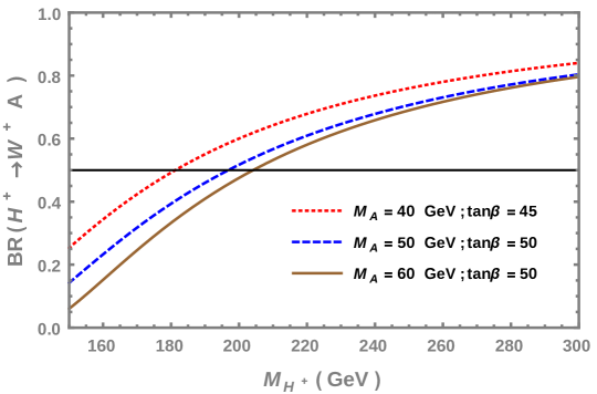
Figure 1: BR($H^{\pm}\to W^{\pm}A$) vs. $M_{H^{\pm}}$ for $M_{A}=40,~{}50~{}{\rm and}~{}60$ GeV. The horizontal line represents the 50% branching ratio.

Our benchmark points include three values of the pseudoscalar mass, namely, $M_{A}=40,~{}50~{}{\rm and}~{}60$ GeV. For each value of $M_{A}$ we vary the charged Higgs mass in the range $150<M_{H^{\pm}}<300$ GeV. We tune the value of $\tan\beta$ and $\cos(\beta-\alpha)$ to respect the constraints from $(g-2)_{\mu}$ and BR($h\to AA$). In the given range for $M_{H^{\pm}}$, $H^{\pm}\to W^{\pm}A$ and $H^{\pm}\to\tau^{+}\nu_{\tau}$ are the two dominant modes. Of these two decay modes, the branching ratio for $H^{\pm}\to W^{\pm}A$ depends on $M_{H^{\pm}},~{}M_{A}$ and $M_{W}$ but not on tan $\beta$. However, BR($H^{\pm}\to\tau^{+}\nu_{\tau}$) is proportional to $M_{H^{\pm}}{\rm tan}^{2}~{}\beta$ Chun et al. (2015). Respecting the constraints from lepton universality and muon $(g-2)$ Chun and Kim (2016), higher tan $\beta$ values are allowed but increasing tan $\beta$ would cause $H^{\pm}\to\tau^{+}\nu_{\tau}$ to win against the $H^{\pm}\to W^{\pm}A$ channel. Keeping this in mind we tune the value of tan $\beta$ for the different values of $M_{A}$ so as to simultaneously satisfy all the constraints and have BR($H^{\pm}\to W^{\pm}A$) $>$ BR($H^{\pm}\to\tau^{+}\nu_{\tau}$). Figure 1 shows a variation of BR($H^{\pm}\to W^{\pm}A$) with $M_{H^{\pm}}$ for $M_{A}=40,~{}50~{}{\rm and}~{}60$ GeV.

3.1 Backgrounds

The major contributions to the SM background for our final state $\mu^{+}\mu^{-}\ 2j\ j_{\tau}$ come from (a) $pp\to\mu^{+}\mu^{-}+jets$, (b) $pp\to t\bar{t}+jets$ and (c) $pp\to VV+jets(V=Z,W,\gamma^{*})$. Of these (a) is the most dominant background having contributions from both the on-shell $Z$ as well as the off-shell photon ($\gamma*$) continuum. This is followed by (b) and (c). All the background events are generated with two additional partons and the events are matched up to two jets using MLM matching scheme Mangano et al. (2007); Hoeche et al. (2005) using the shower-kT algorithm with $p_{T}$ ordered showers. We have used relevant k-factors to account for the QCD radiative corrections to the SM subprocesses. Apart from the above three subprocesses, $tW+jets$ could also contribute to the SM background. However, its contribution was found to be negligible as compared to (a) and (b) background channels, and is therefore ignored in the analysis.

3.2 Simulation and event selection

Signal and background events have been simulated with MadGraph5_aMC@NLO Alwall et al. (2011, 2014) fed to PYTHIA6 Sjostrand et al. (2006) for the subsequent decay, showering and hadronization of the parton level events. $\tau$ decays are incorporated via TAUOLA Jadach et al. (1993) integrated in MadGraph5_aMC@NLO. Event generation uses the NN23LO1 Ball et al. (2015) parton distribution function and the default dynamic renormalisation and factorisation scales mad in MadGraph5_aMC@NLO. Finally, detector simulation is incorporated in Delphes3 de Favereau et al. (2014) using the anti-kT algorithm Cacciari et al. (2008) for jet reconstruction with $R=0.4$. In Delphes3, the $\tau$-tagging efficiency and mistagging efficiencies of the light jets as $\tau$-jets are chosen to be the “Medium tag point” as quoted in ATL (2015). This entails the tagging efficiency of 1-prong (3-prong) $\tau$ decay to be 70% (60%) and the corresponding mistagging rate is 1% (2%).

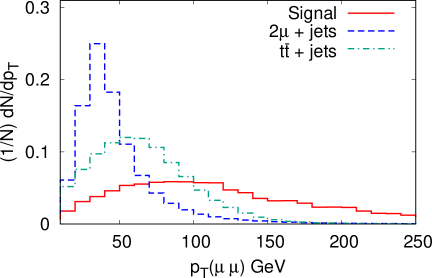
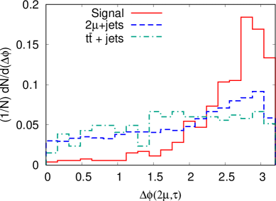
Figure 2: In the left panel we show the $p_{T}\,(\mu\mu)$ distribution for the signal and background. In the right panel we show the azimuthal angle separation between the muon pair and the highest $p_{T}\,\,\tau$-tagged jet.

We use the following selection cuts to select our signal and reduce the accompanying backgrounds:

• Preselection Cuts (a) : We require the final state to have two oppositely charged muons with $p_{T}>10$ GeV accompanied with two light jets and at least one tau-tagged jet of $p_{T}>20$ GeV.

• Preselection Cuts (b) : We also demand a $b$-veto on the final state. This helps to suppress the $t\bar{t}+jets$ and $tW+jets$ background.

• The invariant mass of the di-muon system ($M_{\mu\mu}$) satisfies $|M_{\mu\mu}~{}-~{}M_{A}|<2.5\textrm{ GeV}$.

• The $p_{T}$ of the muon pair has a minimum threshold of $p_{T}(\mu\mu)>90$ GeV. This is chosen keeping in mind that the muons coming from the $A$ decay, which in turn comes from the $H^{\pm}$ or $H$ decay, are expected to be boosted. The transverse momentum distribution of the muon system is depicted in left panel of Figure 2. The signal events are generated with $M_{A}=50$ GeV and $M_{H^{\pm}/H}=210$ GeV. It is evident from the Figure that a cut of 90 GeV on $p_{T}(\mu\mu)$ will suppress the background considerably.

• Finally we also impose a minimum azimuthal separation between the muon pair and the hardest tau-tagged jet, $i.e.$ $\Delta\phi_{2\mu,j_{\tau}}>1.6$. This is because the muon pair and the tau-tagged jet are expected to arise from the decays of $H^{\pm}$ and the associated $A$ respectively. Thus they are expected to have a large azimuthal separation since $H^{\pm}$ and $A$ are expected to be almost back to back and therefore well separated. This is depicted in right panel of Figure 2. It is evident that a cut on $\Delta\phi_{2\mu,j_{\tau}}$ will reduce substantial amount of the background.

Note that the leading dijet system in our analysis is also expected to satisfy an invariant mass window of $|M_{j_{1}j_{2}}-85.0|<20.0$ GeV about the $W$ or $Z$ resonance, which helps us in reconstructing the heavy Higgs mass.

4 Results and Discussion

Cuts	Signal		Background		Significance
	$H^{\pm}A$	$HA$	$\mu^{+}\mu^{-}$+jets	$t\bar{t}$+jets
Preselection Cuts (a)	179	79	38610	25424	1.0
Preselection Cuts (b)	173	72	37755	10125	1.1
$|M_{\mu\mu}-M_{A}|<2.5$ GeV	151	63	9228	2444	2.0
$p_{T}(\mu\mu)>90$ GeV	108	44	2351	605	2.8
$\Delta\Phi(\mu\mu,j_{\tau})>1.6$	98	40	1742	354	3.0

Table 2: Cut flow table displaying effectiveness of different cuts used to enhance signal to background ratio. Signal events are generated with $M_{H^{\pm}}=M_{H}=210$ GeV and $M_{A}=50$ GeV. All the events are estimated with integrated luminosity of $3000fb^{-1}$ data.

In the previous sections we discussed the analysis framework and simulation cuts which can be utilized to improve the signal to background ratio. To quantify the efficacy of different cuts, we consider a benchmark point with $M_{A}=50$ GeV and $M_{H^{\pm}}=M_{H}=210$ GeV and step-by-step cut flow is presented in Table 2. The events are estimated with an integrated luminosity of 3000 $fb^{-1}$. Production cross-section for a 210 GeV charged and neutral Higgs along with a 50 GeV pseudoscalar is 120 fb and 60 fb respectively.

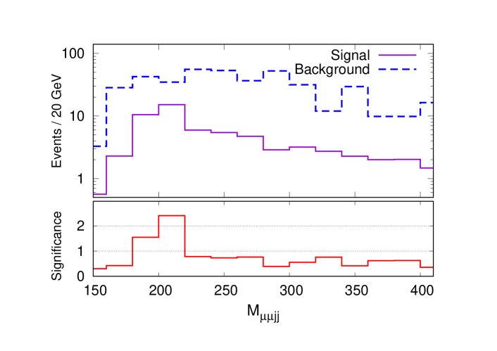
Figure 3: Invariant mass distribution of $\mu^{+}\,\mu^{-}\,j\,j$ system for signal and background events. Signal event are generated for heavy scalar mass of 210 GeV with $M_{A}=50$GeV. The bottom panel shows the binwise significance of the signal comparing the total events to the estimated background events in each invariant mass bin.

With these cuts we have analyze the signal $(S)$ and background events $(B)$, and present the corresponding statistical significance $(\mathcal{S})$ at each step in the right most column. We estimate the significance using the expression:

$$\mathcal{S}=\sqrt{2\left[(S+B)~{}\textrm{ln}\left(1+\frac{S}{B}\right)-S\right]}.$$ (10)

It is clear from the event counts in Table 2 that a search for charged Higgs in the mass range of 200 GeV in Type X 2HDM will be quite challenging. A prior knowledge of the pseudoscalar mass, which in our case is motivated by $(g-2)_{\mu}$ data, enables us to devise specific selection criteria that helps us achieve only a reasonable significance ($\sim 3\sigma$) for its observation. We now aim to reconstruct the mass of the charged Higgs with enough confidence in that particular mass window. To do this, we have plotted the invariant mass distribution of $\mu\,\mu\,j\,j$ system for the signal and background events in Figure 3. Note that for signal events, we have merged events coming from both the charged Higgs and heavy neutral Higgs production channels. The ’Background’ events represent the sum of $t\bar{t}+\,jets$ and $2\mu+\,jets$ processes. The signal events are generated for heavy scalar mass of 210 GeV with $M_{A}=50$ GeV. In the bottom panel of Figure 3 we show the local significance calculated for each bin of the invariant mass using the total events to the estimated background events in each such bin. Although the actual event shapes of the signal and background in the invariant mass distribution when combined may not give a clear indication of a significant resonant behavior, the local significance does indicate a clear peak at 210 GeV (mass of heavy scalars) at a robust $\simeq 2.2\sigma$.

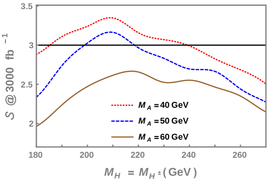
Figure 4: Significance vs. $M_{H^{\pm}}$ for $M_{A}=40,~{}50~{}{\rm and}~{}60$ GeV. The horizontal line represents the 3$\sigma$ limit.

Now to explore a more general parameter space in $M_{H^{\pm}}-M_{A}$ plane, we vary the charged Higgs mass from 180 GeV to 270 GeV and estimate their signal significance. To arrest the effect of the pseudoscalar mass, we have analyzed the signal for three different values of the pseudoscalar mass, viz. 40 GeV, 50 GeV and 60 GeV for every choice of the charged Higgs mass. Using the same cuts as described in Table 2 we have estimated the signal significance at 14 TeV LHC with an integrated luminosity of 3000 $fb^{-1}$. The variation of the statistical significance as a function of $M_{H^{\pm}}$ for different values of $M_{A}$ is shown in Figure 4. As the charged Higgs mass increases, the cross section decreases leading to lower significance and the same observation is true for pseudoscalar mass. Although the production cross-section is higher for light charged Higgs, the branching of $H^{\pm}$ to $W^{\pm}A$ is low (see Figure 1) which effectively decreases the overall significance. We find that the best significance is achieved for moderate values of charged Higgs mass i.e. around 200 - 220 GeV where the production cross-section is not very low while the branching ratio ($H^{\pm}\to W^{\pm}A$) is reasonably large. Thus it would definitely benefit the charged Higgs search in Type X 2HDM if LHC were to accumulate more data than the 3000 $fb^{-1}$ .

5 Summary and Conclusion

We have succesfully demonstrated the reconstructability of the charged and heavy neutral Higgs within the Type-X 2HDM scenario, under the assumption of degeneracy of $M_{H^{\pm}}$ and $M_{H}$. In considering the channel $p~{}p\to H^{\pm}A$, and subsequent decays of $H^{\pm}\to W^{\pm}A,\,\,W^{\pm}\to jj$, with $A\to\mu^{+}\mu^{-}~{}{\rm or}~{}\tau^{+}\tau^{-}$, we have taken advantage of the favourable branching ratio of $H^{\pm}\to W^{\pm}A$ for heavier $H^{\pm}$. We have investigated the kinematic cuts that can help in suppressing the dominant backgrounds to our final state. To this end, the sharp invariant mass peak of the di-muon system around the pseudoscalar mass and a tight $p_{T}$ threshold on the muon pair is found to be effective in containing the $2\mu+jets$ and $t\bar{t}+jets$ backgrounds. In addition, invariant mass window on the dijet system around the electroweak gauge boson masses also helps in the reconstruction of the heavy charged Higgs mass. The contribution coming from the heavy neutral Higgs production to our signal yield is found to be relevant as it happens to be nearly half of that of the charged Higgs production for the given selection criteria. It is seen that with the increase in the mass of the pseudoscalar from 40 to 60 GeV, the statistical significance diminishes and a heavy charged Higgs in the mass range of 200-220 GeV with $M_{A}=40$ GeV has the maximum discovery potential. The analysis projects a significance of $\gtrsim 3\sigma$ for 3000 $fb^{-1}$ for the above benchmark scenario, which can further improve with a possible luminosity upgrade in the 14 TeV run. For example, 5000 $fb^{-1}$ may hike the significance close to about 4 $\sigma$.

6 Acknowledgements

We thank Nabarun Chakrabarty for helpful discussions. This work was partially supported by funding available from the Department of Atomic Energy, Government of India, for the Regional Centre for Accelerator-based Particle Physics (RECAPP), Harish-Chandra Research Institute. We also acknowledge the use of the cluster computing setup available at RECAPP and at the High Performance Computing facility of HRI. EJC thanks RECAPP for hospitality where part of the project was finalized. BM thanks Korea Institute for Advanced Study for hospitality while this project was initiated.

References

- Gunion et al. (2000) J. F. Gunion, H. E. Haber, G. L. Kane, and S. Dawson, Front. Phys. 80, 1 (2000).
- Djouadi (2008) A. Djouadi, Phys. Rept. 459, 1 (2008), hep-ph/0503173.
- Branco et al. (2012) G. C. Branco, P. M. Ferreira, L. Lavoura, M. N. Rebelo, M. Sher, and J. P. Silva, Phys. Rept. 516, 1 (2012), 1106.0034.
- Brown et al. (2001) H. N. Brown et al. (Muon g-2), Phys. Rev. Lett. 86, 2227 (2001), hep-ex/0102017.
- Bennett et al. (2006) G. W. Bennett et al. (Muon g-2), Phys. Rev. D73, 072003 (2006), hep-ex/0602035.
- Cheung et al. (2001) K.-m. Cheung, C.-H. Chou, and O. C. W. Kong, Phys. Rev. D64, 111301 (2001), hep-ph/0103183.
- Cheung and Kong (2003) K. Cheung and O. C. W. Kong, Phys. Rev. D68, 053003 (2003), hep-ph/0302111.
- Jegerlehner and Nyffeler (2009) F. Jegerlehner and A. Nyffeler, Phys. Rept. 477, 1 (2009), 0902.3360.
- Broggio et al. (2014) A. Broggio, E. J. Chun, M. Passera, K. M. Patel, and S. K. Vempati, JHEP 11, 058 (2014), 1409.3199.
- Chun et al. (2015) E. J. Chun, Z. Kang, M. Takeuchi, and Y.-L. S. Tsai, JHEP 11, 099 (2015), 1507.08067.
- Kanemura et al. (2014a) S. Kanemura, H. Yokoya, and Y.-J. Zheng, Nucl. Phys. B886, 524 (2014a), 1404.5835.
- Chun and Kim (2016) E. J. Chun and J. Kim, JHEP 07, 110 (2016), 1605.06298.
- Su and Thomas (2009) S. Su and B. Thomas, Phys. Rev. D79, 095014 (2009), 0903.0667.
- Kanemura et al. (2012) S. Kanemura, K. Tsumura, and H. Yokoya, Phys. Rev. D85, 095001 (2012), 1111.6089.
- Kanemura et al. (2014b) S. Kanemura, K. Tsumura, K. Yagyu, and H. Yokoya, Phys. Rev. D90, 075001 (2014b), 1406.3294.
- Chun et al. (2017) E. J. Chun, S. Dwivedi, T. Mondal, and B. Mukhopadhyaya, Phys. Lett. B774, 20 (2017), 1707.07928.
- Glashow and Weinberg (1977) S. L. Glashow and S. Weinberg, Phys. Rev. D 15, 1958 (1977), URL https://link.aps.org/doi/10.1103/PhysRevD.15.1958.
- Gunion and Haber (2003) J. F. Gunion and H. E. Haber, Phys. Rev. D67, 075019 (2003), hep-ph/0207010.
- Heister et al. (2002) A. Heister et al. (ALEPH), Phys. Lett. B543, 1 (2002), hep-ex/0207054.
- Abdesselam et al. (2016) A. Abdesselam et al. (Belle), in Proceedings, 38th International Conference on High Energy Physics (ICHEP 2016): Chicago, IL, USA, August 3-10, 2016 (2016), 1608.02344, URL https://inspirehep.net/record/1479946/files/arXiv:1608.02344.pdf.
- Wang and Han (2015) L. Wang and X.-F. Han, JHEP 05, 039 (2015), 1412.4874.
- Sirunyan et al. (2018) A. M. Sirunyan et al. (CMS Collaboration), Tech. Rep. CMS-HIG-17-029-003, CERN, Geneva (2018), URL http://cds.cern.ch/record/2317389.
- Mangano et al. (2007) M. L. Mangano, M. Moretti, F. Piccinini, and M. Treccani, JHEP 01, 013 (2007), hep-ph/0611129.
- Hoeche et al. (2005) S. Hoeche, F. Krauss, N. Lavesson, L. Lonnblad, M. Mangano, A. Schalicke, and S. Schumann, in HERA and the LHC: A Workshop on the implications of HERA for LHC physics: Proceedings Part A (2005), pp. 288–289, hep-ph/0602031, URL http://inspirehep.net/record/709818/files/arXiv:hep-ph_0602031.pdf.
- Alwall et al. (2011) J. Alwall, M. Herquet, F. Maltoni, O. Mattelaer, and T. Stelzer, JHEP 06, 128 (2011), 1106.0522.
- Alwall et al. (2014) J. Alwall, R. Frederix, S. Frixione, V. Hirschi, F. Maltoni, O. Mattelaer, H. S. Shao, T. Stelzer, P. Torrielli, and M. Zaro, JHEP 07, 079 (2014), 1405.0301.
- Sjostrand et al. (2006) T. Sjostrand, S. Mrenna, and P. Z. Skands, JHEP 05, 026 (2006), hep-ph/0603175.
- Jadach et al. (1993) S. Jadach, Z. Was, R. Decker, and J. H. Kuhn, Comput. Phys. Commun. 76, 361 (1993).
- Ball et al. (2015) R. D. Ball et al. (NNPDF), JHEP 04, 040 (2015), 1410.8849.
- (30) "http://cp3.irmp.ucl.ac.be/projects/madgraph/wiki/FAQ-General-13".
- de Favereau et al. (2014) J. de Favereau, C. Delaere, P. Demin, A. Giammanco, V. Lemaître, A. Mertens, and M. Selvaggi (DELPHES 3), JHEP 02, 057 (2014), 1307.6346.
- Cacciari et al. (2008) M. Cacciari, G. P. Salam, and G. Soyez, JHEP 04, 063 (2008), 0802.1189.
- ATL (2015) Tech. Rep. ATL-PHYS-PUB-2015-045, CERN, Geneva (2015), URL https://cds.cern.ch/record/2064383.