Matching Parton Showers and Matrix Elements

Abstract

We compare different procedures for combining fixed-order tree-level matrix element generators with parton showers. We use the case of W-production at the Tevatron and the LHC to compare different implementations of the so-called CKKW scheme and one based on the so-called MLM scheme using different matrix element generators and different parton cascades. We find that although similar results are obtained in all cases, there are important differences.

1 Introduction

One of the most striking features of LHC final states will be the large number of events with several hard jets. Final states with 6 jets from $t\bar{t}$ decays will have a rate of almost 1Hz, with 10-100 times more coming from prompt QCD processes. The immense amount of available phase-space, and the large acceptance of the detectors, with calorimeters covering a region of almost 10 units of pseudorapidity ($\eta$), will lead to production and identification of final states with 10 or more jets. These events will hide or strongly modify all possible signals of new physics which involve the chain decay of heavy coloured particles, such as squarks, gluinos or the heavier partners of the top which appear in little-Higgs models. Being able to predict their features is therefore essential.

To achieve this, our calculations need to describe as accurately as possible both the full matrix elements for the underlying hard processes, as well as the subsequent development of the hard partons into jets of hadrons. For the complex final-state topologies we are interested in, no factorization theorem exists however to rigorously separate these two components, providing a constructive algorithm for the implementation of such separation. The main obstacle is the existence of several hard scales, like the jet transverse energies and dijet invariant masses, which for a generic multijet event will span a wide range. This makes it difficult to unambiguously separate the components of the event which belong to the “hard process” (to be calculated using a multiparton amplitude) from those developing during its evolution (described by the parton shower). A given $(N+1)$-jet event can be obtained in two ways: from the collinear/soft-radiation evolution of an appropriate $(N+1)$-parton final state, or from an $N$-parton configuration where hard, large-angle emission during its evolution leads to the extra jet. A factorization prescription (in this context this is often called a “matching scheme”) defines, on an event-by-event basis, which of the two paths should be followed. The primary goal of a matching scheme is therefore to avoid double counting (by preventing some events to appear twice, once for each path), as well as dead regions (by ensuring that each configuration is generated by at least one of the allowed paths). Furthermore, a good matching scheme will optimize the choice of the path, using the one which guarantees the best possible approximation to a given kinematics. It is possible to consider therefore different matching schemes, all avoiding the double counting and dead regions, but leading to different results in view of the different ways the calculation is distributed between the matrix element and the shower evolution. As in any factorization scheme, the physics is independent of the separation between phases only if we have complete control over the perturbative expansion. Otherwise a residual scheme-dependence is left. Exploring different matching schemes is therefore crucial to assess the systematic uncertainties of multijet calculations.

In this work we present a first comparison of the three approaches which have been proposed so far, the so-called CKKW scheme, the Lönnblad scheme, and the MLM scheme. After shortly reviewing them, we present predictions for a set of $W$+multijet distributions at the Tevatron collider and at the LHC.

2 Matching procedures

In general, the different merging procedures all follow a similar strategy:

1. A jet measure is defined and all relevant cross sections including jets are calculated for the process under consideration. I.e. for the production of a final state $X$ in $pp$-collisions, the cross sections for the processes $pp\to X+n\mbox{\rm jets}$ with $n=0,\,1,\,\dots n_{\rm max}$ are evaluated.

2. Hard parton samples are produced with a probability proportional to the respective total cross section, in a corresponding kinematic configuration following the matrix element.

3. The individual configurations are accepted or rejected with a dynamical, kinematics-dependent probability that includes both effects of running coupling constants and of Sudakov effects. In case the event is rejected, step 2 is repeated, i.e. a new parton sample is selected, possibly with a new number of jets.

4. The parton shower is invoked with suitable initial conditions for each of the legs. In some cases, like, e.g. in the MLM procedure described below, this step is performed together with the step before, i.e. the acceptance/rejection of the jet configuration. In all cases the parton shower is constrained not to produce any extra jet; stated in other words: Configurations that would fall into the realm of matrix elements with a higher jet multiplicity are vetoed in the parton shower step.

From the description above it is clear that the merging procedures discussed in this contribution differ mainly

• in the jet definition used in the matrix elements;

• in the way the acceptance/rejection of jet configurations stemming from the matrix element is performed;

• and in details concerning the starting conditions of and the jet vetoing inside the parton showering.

2.1 CKKW

In the original merging description according to [1, 2], which has been implemented [3] in S HERPA [4] in full generality, the acceptance/rejection of jet configurations from the matrix elements and the parton showering step are well-separated.

In this realisation of what is known as the CKKW-prescription the phase space separation for the different multijet processes is achieved through a $k_{\perp}$-measure [5, 6, 7]. For the case of hadron–hadron collisions, two final-state particles belong to two different jets, if their relative transverse momentum

$$k_{\perp}^{(ij)2}=2\,\mbox{\rm min}\left\{p_{\perp}^{(i)},\,p_{\perp}^{(j)}\right\}^{2}\left[\cosh(\eta^{(i)}-\eta^{(j)})-\cos(\phi^{(i)}-\phi^{(j)})\right]$$ (1)

is larger than a critical value, $k^{2}_{\perp,0}$. In addition, the transverse momentum of each jet has to be larger than $k_{\perp,0}$. The matrix elements are then reweighted by appropriate Sudakov and coupling weights. The task of the weight attached to a matrix element is to take into account terms that would appear in a corresponding parton shower evolution. Therefore, a “shower history” is reconstructed by clustering the initial and final state partons according to the $k_{\perp}$-algorithm. The resulting chain of nodal $k_{\perp}$-measures is interpreted as the sequence of relative transverse momenta of multiple jet production. The first ingredient of the weight are the strong coupling constants taken at the respective nodal values, divided by the value of $\alpha_{S}$ used during the matrix element evaluation. The other part of the correction weight is provided by NLL-Sudakov form factors defined by

$$\Delta_{q,g}(Q,Q_{0}):=\exp\left[-\int\limits_{Q_{0}}^{Q}\mbox{\rm d}q\Gamma_{q,g}(Q,q)\right]\,,$$ (2)

where the integrated splitting functions $\Gamma_{q,g}$ are given by

$$\Gamma_{q,g}(Q,q):=\left\{\begin{array}[]{l}\frac{2C_{F}\alpha_{s}(q)}{\pi q}\left[\log\frac{Q}{q}-\frac{3}{4}\right]\\ \frac{2C_{A}\alpha_{s}(q)}{\pi q}\left[\log\frac{Q}{q}-\frac{11}{12}\right]\end{array}\right.$$ (3)

and contain the running coupling constant and the two leading, logarithmically enhanced terms in the limit when $Q_{0}\ll Q$. The two finite, non-logarithmic terms $-3/4$ and $-11/12$, respectively emerge when integrating the non-singular part of the corresponding splitting function in the limits $[0,\,1]$. Potentially, when $q/Q$ is not going to zero, these finite terms are larger than the logarithmic terms and thus spoil an interpretation of the emerging NLL-Sudakov form factor as a non-branching probability. Therefore, without affecting the logarithmic order of the Sudakov form factors, these finite terms are integrated over the interval $[q/Q,\,1-q/Q]$ rather than over $[q,\,Q]$. This way a Sudakov form factor determines the probability for having no emission resolvable at scale $Q_{0}$ during the evolution from a higher scale $Q$ to a lower scale $Q_{0}$. A ratio of two Sudakov form factors $\Delta(Q,Q_{0})/\Delta(q,Q_{0})$ then gives the probability for having no emission resolvable at scale $Q_{0}$ during the evolution from $Q$ to $q$. Having reweighted the matrix element, a smooth transition between this and the parton shower region is achieved by choosing suitable starting conditions for the shower evolution of the parton ensemble and vetoing any parton shower emission that is harder than the separation cut $k_{\perp,0}$.

Within S HERPA  the required matrix elements are provided by its internal matrix element generator AMEGIC++ [8] and the parton shower phase is handled by APACIC++ [9, 10]. Beyond the comparisons presented here the S HERPA predictions for $W$+multijets have already been validated and studied for Tevatron and LHC energies in [11, 12]. Results for the production of pairs of $W$-bosons have been presented in [13].

2.2 The Dipole Cascade and CKKW

The dipole model[14, 15] as implemented in the A RIADNE program[16] is based around iterating $2\rightarrow 3$ partonic splitting instead of the usual $1\rightarrow 2$ partonic splittings in a conventional parton shower. Gluon radiation is modeled as being radiated coherently from a color–anticolor charged parton pair. This has the advantage of eg. including first order correction to the matrix elements for $e^{+}e^{-}\to q\bar{q}$ in a natural way and it also automatically includes the coherence effects modeled by angular ordering in conventional showers. The process of quark antiquark production does not come in as naturally, but can be added[17]. The emissions in the dipole cascade is ordered according to invariant transverse momentum defined as

$$p_{\perp}^{2}=\frac{s_{12}s_{23}}{s_{123}},$$ (4)

where $s_{ij}$ is the squared invariant mass of parton $i$ and $j$, with the emitted parton having index 2.

When applied to hadronic collisions, the dipole model does not separate between initial and final state radiation. Instead all emissions are treated as coming from final state dipoles[18, 19]. To be able to extend the dipole model to hadron collisions, extended colored objects are introduced to model the hadron remnants. Dipoles involving hadron remnants are treated in a similar manner to the normal final-state dipoles. However, since the hadron remnant is considered to be an extended object, emissions with small wavelength are suppressed. This is modeled by only letting a fraction of the remnant take part in the emission. The fraction that is resolved during the emission is given by

$$a(p_{\perp})=\left(\frac{\mu}{p_{\perp}}\right)^{\alpha},$$ (5)

where $\mu$ is the inverse size of the remnant and $\alpha$ is the dimensionality.

There are two additional forms of emissions which need to be included in the case of hadronic collisions. One corresponds to an initial state $g\rightarrow q\bar{q}$[20]. This does not come in naturally in the dipole model, but is added by hand in a way similar to that of a conventional initial-state parton shower[20]. The other corresponds to the initial-state $q\to gq$ (with the gluon entering into the hard sub-process) which could be added in a similar way, but this has not been implemented in A RIADNE yet.

When implementing CKKW for the dipole cascade, the procedure is slightly different from what has been described above[21, 22]. First, rather than just reconstructing emission scales using the $k_{\perp}$-algorithm, a complete dipole shower history is constructed for each state produced by the Matrix Element generator, basically answering the question how would A RIADNE have generated this state. This will produce a complete set of intermediate partonic states, $S_{i}$, and the corresponding emission scales, $p_{\perp i}$.

The Sudakov form factors are then introduced using the Sudakov veto algorithm. The idea is that we want to reproduce the Sudakov form factors used in Ariadne. This is done by performing a trial emission starting from each intermediate state $S_{i}$ with $p_{\perp i}$ as a starting scale. If the emitted parton has a $p_{\perp}$ higher than $p_{\perp i+1}$ the state is rejected. This correspond to keeping the state according to the no emission probability in Ariadne, which is exactly the Sudakov form factor.

It should be noted that for initial-state showers, there are two alternative ways of defining the Sudakov form factor. The definition in eq. (2) is used in eg.  HERWIG [23], while eg. P YTHIA [24, 25] uses a form which includes ratios of parton densities. Although formally equivalent to leading logarithmic accuracy, only the latter corresponds exactly to a no-emission probability, and this is the one generated by the Sudakov-veto algorithm. This, however, also means that the reconstructed emissions need not only be reweighted by the running $\alpha_{S}$ as in the standard CKKW procedure above, but also with ratios of parton densities, which in the case of gluon emissions correspond to the suppression due to the extended remnants in eq. (5) as explained in more detail in [22], where the complete algorithm is presented.

2.3 The MLM proceedure

In this approach we match the partons from the ME calculation to the jets reconstructed after the perturbative shower. Parton-level events are defined by a minimum $E_{T}$ threshold $E_{T}^{min}$ for the partons, and a minimum separation among them, $\Delta R_{jj}>R_{min}$. A tree structure is defined in analogy with the CKKW algorithm, starting however from the colour-flow extracted from the matrix-element calculation [26], thus defining the scales at which the various powers of $\alpha_{s}$ are calculated. However, no Sudakov reweighting is applied. Rather, events are showered, without any hard-emission veto during the shower. After evolution, a jet cone algorithm with cone size $R_{min}$ and minimum transverse energy $E_{T}^{min}$ is applied to the final state. Starting from the hardest parton, the jet which is closest to it in $(\eta,\phi)$ is selected. If the distance between the parton and the jet centroid is smaller than $R_{min}$, the parton and the jet match. The matched jet is removed from the list of jets, and matching for subsequent partons is performed. The event is fully matched if each parton has a matched jet. Events which do not match are rejected. A typical example is when two partons are so close that they cannot generate independent jets, and therefore cannot match. Rejection removes double counting of the leading double logarithms associated to the collinear behaviour of the amplitude when two partons get close. Another example is when a parton is too soft to generate its own jet, again failing matching. This removes double counting of some single logarithms. For events which satisfy matching, it is furthermore required that no extra jet, in addition to those matching the partons, be present. Events with extra jets are rejected, a suppression replacing the Sudakov reweighting used in the CKKW approach. Events obtained by applying this procedure to the parton level with increasing multiplicity can then be combined to obtain fully inclusive samples spanning a large multiplicity range. Events with extra jets are not rejected in the case of the sample with highest partonic multiplicity. The distributions of observables measured on this inclusive data set should not depend on the value of the parameters $E_{T}^{min}$ and $R_{min}$, similar to the $k_{\perp,0}$ independence of the CKKW approach. This algorithm is encoded in the A LPGEN  generator [27, 28], where evolution with both HERWIG  and P YTHIA  are enabled. In the following studies, the results quoted as “A LPGEN ” employ the MLM matching scheme, and use A LPGEN for the generation of the parton-level matrix elements and HERWIG for the shower evolution and hadronisation.

3 Examples and comparisons

We present in this Section some concrete examples. We concentrate on the case of $W$+multijet production, which is one of the most studied final states because of its important role as a background to top quark studies at the Tevatron. At the LHC, $W$+jets, as well as the similar $Z$+jets processes, will provide the main irreducible backgrounds to signals such as multijet plus missing transverse energy, typical of Supersymmetry and of other manifestations of new physics. The understanding of $W$+multijet production at the Tevatron is therefore an essential step towards the validation and tuning of the tools presented here, prior to their utilization at the LHC.

For each of the three codes we calculated a large set of observables, addressing inclusive properties of the events ($p_{T}$ spectrum of the $W$ and of leading jets), geometric correlations between the jets, and intrinsic properties of the jets themselves, such as energy shapes. In view of the limited space available here we present only a subset of our studies, which will be documented in more detail in a future publication. An independent study of the systematics in the implementation of the CKKW prescription in HERWIG and P YTHIA was documented in [29].

The comparison between the respective results shows a reasonable agreement among the three approaches, but points also to differences, in absolute rates as well as in the shape of individual distributions, which underscore the existence of an underlying systematic uncertainty. The differences are nevertheless by and large consistent with the intrinsic systematic uncertainties of each of the codes, such as the dependence on the generation cuts or on the choice of renormalization scale. There are also differences due to the choice of parton cascade. In particular the A RIADNE cascade is quite different from a conventional parton shower, and it has been shown in this workshop [30] that A RIADNE eg. gives a much harder $p_{\perp\mbox{W}}$ spectrum than does HERWIG or P YTHIA . Now, although the hard emissions in the matching proceedures should be described by the exact matrix element, the Sudakov formfactors in the A RIADNE matching (and indirectly in the MLM scheme) are generated by the cascade. In addition, the events in the A RIADNE matching are reweighted by PDF ratios in the same way as is done in the plain cascade. This means that some properties of the cascade may affect also the hard emissions in the matching procedure in these cases.

The existence in each of the codes of parameters specifying the details of the matching algorithms presents therefore an opportunity to tune each code so as to best describe the data. This tuning should be seen as a prerequisite for a quantitative study of the overall theoretical systematics: after the tuning is performed on a given set of final states (e.g. the $W$+jets considered here), the systematics for other observables or for the extrapolation to the LHC can be obtained by comparing the difference in extrapolation between the various codes. It is therefore auspicable that future analysis of Tevatron data will provide us with spectra corrected for detector effects in a fashion suitable to a direct comparison against theoretical predictions.

The following two sections present results for the Tevatron ($p\bar{p}$ collisions at 1.96 TeV) and for the LHC ($pp$ at 14 TeV), considering events with a positively charged $W$. Jets are defined by Paige’s GETJET cone-clustering algorithm, with a calorimeter segmentation of ($\Delta\eta$, $\Delta\phi$) = (0.1,$6^{\circ}$) and a cone size of 0.7 and 0.4 for Tevatron and LHC, respectively. At the Tevatron (LHC) we consider jets with $E_{T}>10(20)$ GeV, within $|\eta|<2(4.5)$. We use the PDF set CTEQ6L, with $\alpha_{S}(M_{Z})=0.118$.

For our default distributions, the A LPGEN  results for the Tevatron (LHC) were obtained using parton level cuts of $p_{T,min}=10(20)$ GeV, $|\eta|<2.5(5)$, $R{jj}<0.7(0.4)$ and matching defined by $E_{Tmin}=10$ GeV and $R=0.7$. The S HERPA  samples have been generated using matrix elements with up to four extra jets and the value of the merging scale has been chosen to $k_{\perp,0}=10(20)$ GeV, respectively. Finally, for A RIADNE , the parton level cuts were $p_{T,min}=10(20)$, $R{jj}<0.5(0.35)$ and, in addition, a cut on the maximum pseudorapidity of jets, $\eta_{j\max}=2.5(5.0)$.

In all cases, the analysis is done at the hadron level, but without including the underlying event.

3.1 Tevatron Studies

We start by showing in fig. 1 the inclusive $E_{T}$ spectra of the leading 4 jets. The absolute rate predicted by each code is used, in units of pb/GeV. We notice that the A LPGEN spectrum for the first two jets is softer than both S HERPA and A RIADNE , with the latter having even harder tails. The spectra for the third and fourth jet are instead in very good agreement, both in shape and normalization. As an indication of possible sources of systematics in these calculations, we rescaled the renormalization scale used in A LPGEN by a factor of 1/2. As seen in fig. 2 the distributions for the leading jets is now in perfect agreement with S HERPA , with an increase in rate for the third and fourth jet. These plots give us an idea of the level of flexibility which is intrinsic in the calculation of higher-order jet production. One should not forget that the rate for production of $N$ jets is proportional to the $N$th power of $\alpha_{s}$, and the absence of the full set of virtual corrections unavoidably leads to a large scale uncertainty.

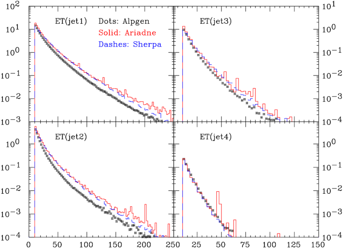
Figure 1: Inclusive $E_{T}$ spectra of the leading 4 jets at the Tevatron (pb/GeV).

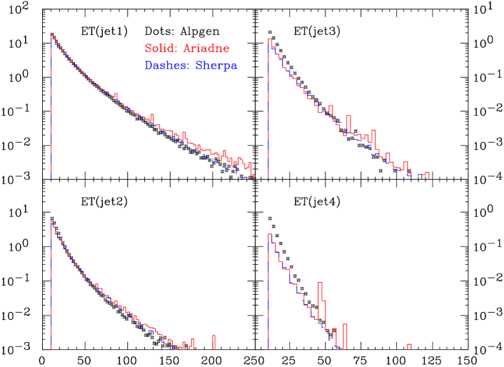
Figure 2: Same as Fig. 1, but with the A

LPGEN

renormalization scale reduced by a factor 2.

Figure 3 shows the inclusive $\eta$ spectra of the leading 4 jets, all normalized to unit area. The asymmetry for the first two jets is due to the $W+$, which preferentially moves in the direction of the proton (positive $\eta$). This is partially washed out in the case of the third and fourth jet. There is a good agreement between the spectra of A LPGEN and S HERPA , while A RIADNE spectra appear to be broader, in particular for the subleading jets. This broadening is expected since the gluon emissions in A RIADNE are essentially unordered in rapidity, which means that the Sudakov form factors applied to the ME-generated states include also a $\log 1/x$ resummation absent in the other programs.

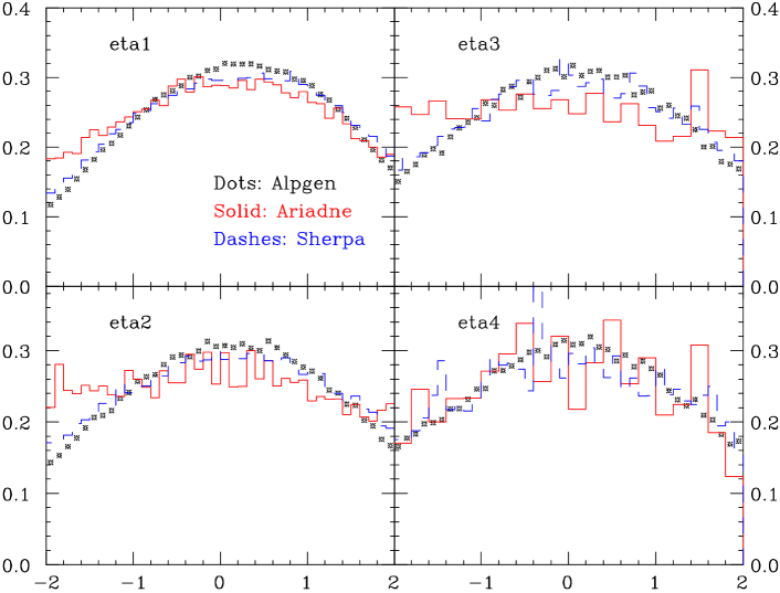
Figure 3: Inclusive $\eta$ spectra of the leading 4 jets at the Tevatron, normalized to unit area.

The top-left plot of fig. 4 shows the inclusive $p_{T}$ distribution of the $W^{+}$ boson, with absolute normalization in pb/GeV. This distribution reflects in part the behaviour observed for the spectrum of the leading jet, with A LPGEN slightly softer, and A RIADNE slightly harder than S HERPA . The $|\eta|$ separation between the $W$ and the leading jet of the event is shown in the top-right plot. The two lower plots show instead the distributions of $|\eta({\mathrm{jet}}_{1})-\eta({\mathrm{jet}}_{2})|$ and $|\eta({\mathrm{jet}}_{2})-\eta({\mathrm{jet}}_{3})|$. These last three plots are normalized to unit area. In all these cases, we observe once more a reflection of the behaviour observed in the inclusive $\eta$ distributions of the jets: A LPGEN is slightly narrower than S HERPA , and A RIADNE is slightly broader.

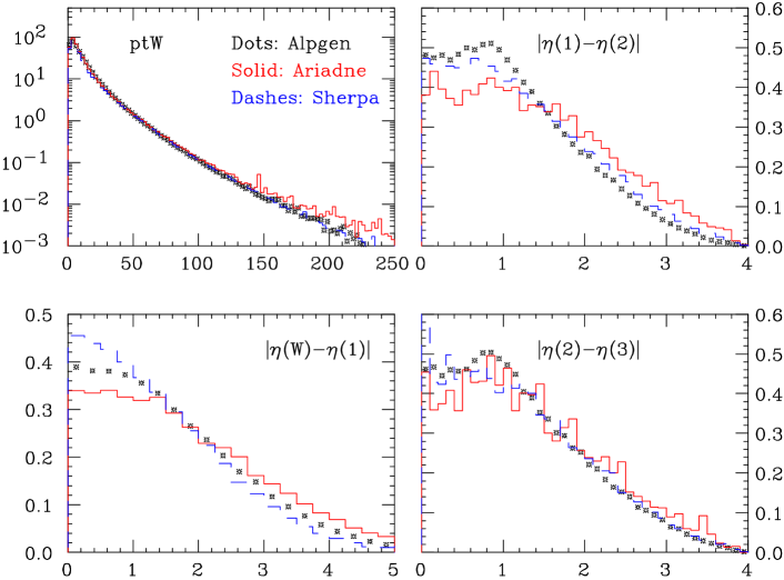
Figure 4: Top left: inclusive $p_{\perp}(W^{+})$ spectrum, pb/GeV. Bottom left: $|\eta(W^{+})-\eta({\mathrm{jet}}_{1})|$ (unit area). Top right: $|\eta({\mathrm{jet}}_{1})-\eta({\mathrm{jet}}_{2})|$ and bottom right: $|\eta({\mathrm{jet}}_{2})-\eta({\mathrm{jet}}_{3})|$ (unit area).

3.2 LHC Predictions

In this section we confine ourselves to A LPGEN and S HERPA . It turns out that A RIADNE has a problem in the reweighting related to the fact that initial-state $g\to q\bar{q}$ emissions, contrary to the gluon emissions, are ordered both in $p_{\perp}$ and rapidity. With the extra phase space available at the LHC this leads to unnatural reconstructions which, in turn, gives rise to a systematically too high reweighting. A solution for this problem is under investigation and a fuller comparison including A RIADNE will be documented in a future publication.

Following the same sequence of the Tevatron study, we start by showing in fig. 5 the inclusive $E_{T}$ spectra of the leading 4 jets. The absolute rate predicted by each code is used, in units of pb/GeV. The relative behaviour of the predictions by A LPGEN and S HERPA follows the pattern observed in the Tevatron case, with A LPGEN being softer in the case of the leading two jets. We do not notice however a deterioration of the discrepancy going from the Tevatron to the LHC, suggesting that once a proper tuning is achieved at lower energy the predictions of two codes for the LHC should be comparable.

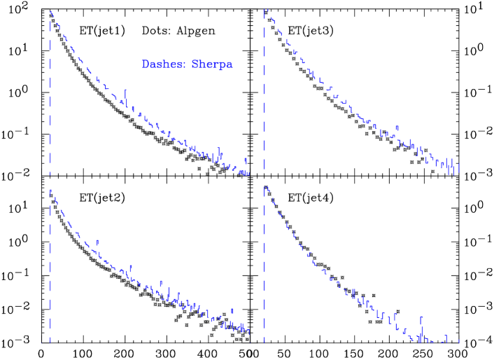
Figure 5: Inclusive $E_{T}$ spectra of the leading 4 jets at the LHC (pb/GeV).

Figure 6 shows the inclusive $\eta$ spectra of the leading 4 jets, all normalized to unit area. The asymmetry now is not present, because of the symmetric rapidity distribution of the $W^{+}$ in $pp$ collisions. As in the case of the Tevatorn, jet production in A LPGEN is slightly more central than in S HERPA .

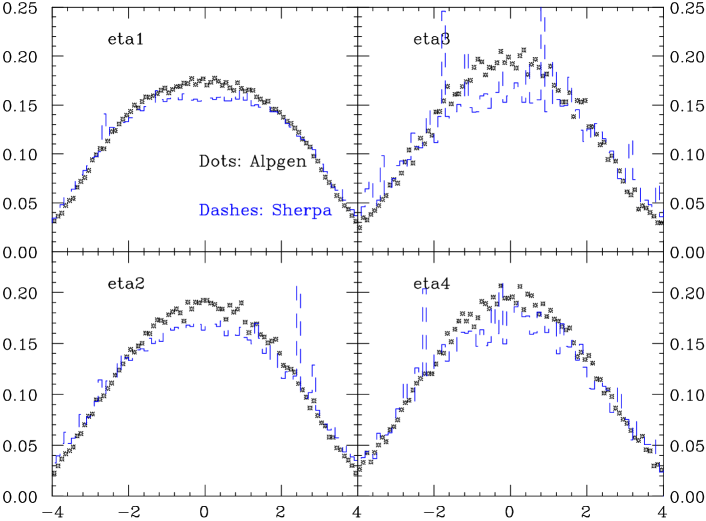
Figure 6: Inclusive $\eta$ spectra of the leading 4 jets at the LHC, normalized to unit area.

The top-left plot of fig. 7 shows the inclusive $p_{T}$ distribution of the $W^{+}$ boson, with absolute normalization in pb/GeV. The $|\eta|$ separation between the $W$ and the leading jet of the event is shown in the top-right plot. The two lower plots show instead the distributions of $|\eta({\mathrm{jet}}_{1})-\eta({\mathrm{jet}}_{2})|$ and $|\eta({\mathrm{jet}}_{2})-\eta({\mathrm{jet}}_{3})|$. These last three plots are normalized to unit area. As before, the features of these comparisons reflect what observed in the inclusive jet properties.

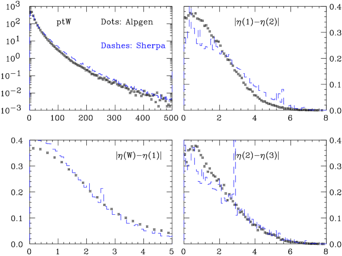
Figure 7: Top left: inclusive $pt_{T}(W^{+})$ spectrum, pb/GeV. Bottom left: $|\eta(W^{+})-\eta({\mathrm{jet}}_{1})|$ (unit area). Top right: $|\eta({\mathrm{jet}}_{1})-\eta({\mathrm{jet}}_{2})|$ and bottom right: $|\eta({\mathrm{jet}}_{2})-\eta({\mathrm{jet}}_{3})|$ (unit area).

4 Conclusions

This document summarizes our study of a preliminary comparison of three independent approaches to the problems of merging matrix element and parton shower evolution for multijet final states. Overall, the picture shows a general consistency between the three approaches, although there are occasional differences. The origin of these differences is under study. It could be based on intrinsic differences between the matching schemes, as well as to differences between the different shower algorithms used in the three cases. We expect nevertheless that these differences be reconciled with appropriate changes in the default parameter settings for the matching schemes, as partly supported by the few systematic studies presented here. Validation and tuning on current Tevatron data is essential, and will allow to reduce the systematics.

It is also important to compare these models to HERA data. However, besides some preliminary investigations for A RIADNE [31], there is no program which properly implement a CKKW or MLM matching scheme for DIS. The energy of HERA is, of course, lower, as are the jet multiplicities and jet energies, but HERA has the advantage of providing a large phase space for jet production which is not mainly determined by the hard scale, $Q^{2}$, but rather by the total energy, giving rise to large logarithms of $x\approx Q^{2}/W^{2}$ which need to be resummed to all orders. This is in contrast to the Tevatron, where the phase space for additional jets in W-production mainly are determined by $m_{W}$. However, when going to the LHC there may also be important effects of the increased energy, and there will be large logarithms of $x\propto m_{W}/\sqrt{S}$ present, which may need to be resummed. The peculiar treatment of the available phase space in the plain A RIADNE cascade means that some logarithms of $x$ are resummed in contrast to conventional initial-state parton cascades. This feature survives the matching procedure and is the reason for the broader rapidity spectra presented in the figures above. In DIS this is reflected by the increased rate of forward jets, and such measurements are known to be well reproduced by A RIADNE while conventional parton showers fail. It would be very interesting if the matching of these conventional showers with higher order matrix elements would improve the description of forward jets. In that case the extrapolation of the Tevatron results to the LHC would be on much safer grounds.

As our study of the LHC distributions suggests, the increase in energy exhibits the same pattern of discrepancies observed at the Tevatron. We therefore expect that if different algorithms are tuned on the same set of data, say Tevatron $W$+jets, they will extrapolate in the same way to the LHC or to different final states, for example multijet configurations without $W$ bosons. While these systematics studies can be performed directly at the Monte Carlo level, only the availability of real measurements from the Tevatron can inject the necessary level or realism in these exploration. We look forward to the availability of such data.

References

- [1] S. Catani, F. Krauss, R. Kuhn, and B. R. Webber, JHEP 0111, 063 (2001). arXiv:hep-ph/0109231
- [2] F. Krauss, JHEP 0208, 015 (2002). arXiv:hep-ph/0205283
- [3] A. Schälicke and F. Krauss, JHEP 07, 018 (2005). hep-ph/0503281
- [4] T. Gleisberg, S. Höche, F. Krauss, A. Schälicke, S. Schumann, and J. Winter, JHEP 0402, 056 (2004). arXiv:hep-ph/0311263
- [5] S. Catani, Y. L. Dokshitser, M. Olsson, G. Turnock, and B. R. Webber, Phys. Lett. B 269, 432 (1991)
- [6] S. Catani, Y. L. Dokshitser, and B. R. Webber, Phys. Lett. B 285, 291 (1992)
- [7] S. Catani, Y. L. Dokshitser, and B. R. Webber, Nucl. Phys. B 406, 187 (1993)
- [8] F. Krauss, R. Kuhn, and G. Soff, JHEP 0111, 044 (2002). arXiv:hep-ph/0109036
- [9] R. Kuhn, F. Krauss, B. Ivanyi, and G. Soff, Comput. Phys. Commun. 134, 223 (2001). hep-ph/0004270
- [10] F. Krauss, A. Schälicke, and G. Soff, hep-ph/0503087
- [11] F. Krauss, A. Schälicke, S. Schumann, and G. Soff, Phys. Rev. D70, 114009 (2004). hep-ph/0409106
- [12] F. Krauss, A. Schalicke, S. Schumann, and G. Soff, Phys. Rev. D72, 054017 (2005). hep-ph/0503280
- [13] T. Gleisberg, F. Krauss, A. Schalicke, S. Schumann, and J.-C. Winter, Phys. Rev. D72, 034028 (2005). hep-ph/0504032
- [14] G. Gustafson and U. Pettersson, Nucl. Phys. B306, 746 (1988)
- [15] G. Gustafson, Phys. Lett. B175, 453 (1986)
- [16] L. Lönnblad, Comput. Phys. Commun. 71, 15 (1992)
- [17] B. Andersson, G. Gustafson, and L. Lönnblad, Nucl. Phys. B339, 393 (1990)
- [18] B. Andersson, G. Gustafson, L. Lönnblad, and U. Pettersson, Z. Phys. C43, 625 (1989)
- [19] L. Lönnblad, Nucl. Phys. B458, 215 (1996). hep-ph/9508261
- [20] L. Lönnblad, Z. Phys. C65, 285 (1995)
- [21] L. Lönnblad, JHEP 05, 046 (2002). hep-ph/0112284
- [22] N. Lavesson and L. Lönnblad, JHEP 07, 054 (2005). hep-ph/0503293
- [23] G. Corcella et al., JHEP 01, 010 (2001). hep-ph/0011363
- [24] T. Sjöstrand, and others, Comput. Phys. Commun. 135, 238 (2001). arXiv:hep-ph/0010017
- [25] T. Sjöstrand, L. Lönnblad, S. Mrenna, and P. Skands (2003). hep-ph/0308153
- [26] F. Caravaglios, M. L. Mangano, M. Moretti, and R. Pittau, Nucl. Phys. B539, 215 (1999). hep-ph/9807570
- [27] M. L. Mangano, M. Moretti, and R. Pittau, Nucl. Phys. B632, 343 (2002). hep-ph/0108069
- [28] M. L. Mangano, M. Moretti, F. Piccinini, R. Pittau, and A. D. Polosa, JHEP 07, 001 (2003). hep-ph/0206293
- [29] S. Mrenna and P. Richardson, JHEP 05, 040 (2004). hep-ph/0312274
- [30] B. Kersevan and E. Richter-Was., The Monte Carlo Event Generator AcerMC and package AcderDET. These Proceedings
- [31] C. Åberg, Correcting the colour dipole cascade with fixed order matrix elements in deep inelastic scattering. Diploma thesis, Lund preprint LU-TP 04-25.