Toward realistic simulations of magneto-thermal winds from weakly-ionized protoplanetary disks

Abstract

Protoplanetary disks (PPDs) accrete onto their central T Tauri star via magnetic stresses. When the effect of ambipolar diffusion (AD) is included, and in the presence of a vertical magnetic field, the disk remains laminar between 1-5 au, and a magnetocentrifugal disk wind forms that provides an important mechanism for removing angular momentum. We present global MHD simulations of PPDs that include Ohmic resistivity and AD, where the time-dependent gas-phase electron and ion fractions are computed under FUV and X-ray ionization with a simplified recombination chemistry. To investigate whether the mass loading of the wind is potentially affected by the limited vertical extent of our existing simulations, we attempt to develop a model of a realistic disk atmosphere. To this end, by accounting for stellar irradiation and diffuse reprocessing of radiation, we aim at improving our models towards more realistic thermodynamic properties.

1 Introduction

Interpreting observational properties of T Tauri systems [1] is closely tied to understanding the complex dynamical evolution of gaseous protoplanetary disks (PPDs), both in terms of their chemistry, and in terms of the microphysics that govern the evolution of the embedded magnetic fields. Moreover, with PPDs being the birth sites for extrasolar planets, a sound physical picture of the dust [2] and planetesimal [3] evolution is needed to ultimately provide the building blocks for a comprehensive theory of planet formation.

The fundamental drivers of disk evolution are mass loss processes and redistribution of angular momentum [4]. In sufficiently ionized parts of the disk, the latter can be achieved by turbulent stresses. When accounting for the ionization structure of a typical PPD, large parts of the disk, however, remain laminar owing to the effect of ambipolar diffusion (AD). In this situation, angular momentum is primarily transported via a magnetocentrifugal disk wind [5, 6]. While this picture is further complicated when accounting for the Hall effect [7, 8], it has nevertheless become clear that the thermal structure of the disk plays an important role in setting the mass loading of the disk wind [9], and hence the timescale on which the system evolves [10, 11].

2 Methods

As in our previous work [6], we are solving the single-fluid MHD equations including Ohmic resistivity and ambipolar diffusion, that is, the electromotive force resulting from the mutual collision of ions and neutrals. The diffusion coefficients, $\eta_{\rm O}$, and $\eta_{\rm AD}$ are specified by means of a look-up table, which has been obtained by solving a simple chemical ionization/recombination network. The resulting electromotive forces stemming from the Ohmic and ambipolar diffusion terms are then given by

$$\mathbf{E}_{\rm O}\equiv-\eta_{\rm O}\,(\nabla\!\times\!\mathbf{B})\,,\quad\textrm{and}$$ (1)

$$\mathbf{E}_{\rm AD}\equiv\eta_{\rm AD}\,\left[\,(\nabla\!\times\!\mathbf{B})\times\hat{{\mathbf{b}}}\,\right]\times\hat{{\mathbf{b}}}\,,$$ (2)

with $\hat{{\mathbf{b}}}\equiv\mathbf{B}/|\mathbf{B}|$ being the unit vector along $\mathbf{B}$, and where the double vector product results in an additional minus sign, such that positive coefficients $\eta_{\rm O}$ and $\eta_{\rm AD}$ signify diffusion of magnetic fields, with the latter only being sensitive to currents perpendicular to the field direction.

For the typical number densities in the context of PPDs, the frictional coupling between the ions and neutrals happens so quickly (compared to dynamical timescales of interest) that we assume the charged species move at their terminal velocity with respect to the neutrals, that is, where the Lorentz force is balanced by the drag. Because of the low degree of ionization, we formulate our continuity equation and momentum conservation in terms of the neutral component, although it does experience the Lorentz force as mediated by particle collisions.

We use a modified version of the nirvana-iii finite volume Godunov code [12, 13]. The code adopts a total-energy formulation with conserved variables $\rho$, $\rho\mathbf{v}$, and $e\equiv\epsilon+\rho\mathbf{v}^{2}\!/2+\mathbf{B}^{2}\!/2$. Together with the conservation of radiation energy, $E_{\rm R}$, and defining the total pressure, $p^{\star}$, as the sum of the gas and magnetic pressures, the system of equations we solve reads

$$\partial_{t}\rho+\nabla\!\cdot\!(\rho\mathbf{v}) = 0\,,$$ (3)

$$\partial_{t}(\rho\mathbf{v})+\nabla\!\cdot\!\big{[}\rho\mathbf{vv}+p^{\star}I-\mathbf{BB}\,\big{]} = -\rho\nabla\Phi+\rho\kappa_{\rm R}/c\,\mathbf{F}_{\rm R}\,,$$ (4)

$$\partial_{t}e+\nabla\!\cdot\!\big{[}(e+p^{\star})\mathbf{v}-(\mathbf{v}\!\cdot\!\mathbf{B})\mathbf{B}\,\big{]} = \nabla\cdot\big{[}\,(\mathbf{E}_{\rm O}\!+\!\mathbf{E}_{\rm AD})\!\times\!\mathbf{B}\,\big{]}-\rho(\nabla\Phi)\!\cdot\!\mathbf{v}$$ (5)

$$+\,c\,\rho\kappa_{\rm P}\left(E_{\rm R}-a_{\rm R}\,T^{4}\right)+\rho\kappa_{\rm R}/c\,\mathbf{F}_{\rm R}\!\cdot\!\mathbf{v}+\mathcal{Q}^{+}_{\rm irr}\,,$$

$$\partial_{t}E_{\rm R}+\nabla\!\cdot\!(E_{\rm R}\mathbf{v}) = -\,c\,\rho\kappa_{\rm P}\left(E_{\rm R}-a_{\rm R}\,T^{4}\right)-\nabla\!\cdot\!\mathbf{F}_{\rm R}-\mathcal{P}_{\rm R}\!:\!\nabla\mathbf{v}\,,$$ (6)

$$\partial_{t}\mathbf{B}-\!\nabla\!\times\!\big{[}\,\mathbf{v}\!\times\!\mathbf{B}+\mathbf{E}_{\rm O}+\mathbf{E}_{\rm AD}\,\big{]} = 0\,,$$ (7)

where $\mathbf{F}_{\rm R}$ is the radiation flux, $\mathcal{P}_{\rm R}$ is the radiation pressure tensor, $\kappa_{\rm R}$ and $\kappa_{\rm P}$ are the Rosseland and Planck mean opacities, respectively, $a_{\rm R}\equiv 4\,\sigma/c$ is the radiation density constant, $T\equiv\bar{\mu}m_{\rm H}/k_{\rm B}\;p/\rho$ is the gas temperature, and the gas pressure is $p=(\gamma-1)\epsilon$, where $\gamma=7/5$ is chosen as appropriate for an ideal diatomic gas. The gravitational term $\Phi(r)\equiv-G\,M_{\odot}/r$ represents the point-mass potential of the solar-mass star at the center of our spherical-polar coordinate system, and $\mathcal{Q}^{+}_{\rm irr}$ represents external irradiation heating due to the star.

2.1 Flux limited diffusion

The above equations can only be solved once the radiation flux and pressure tensor are specified. An attractive method for obtaining the Eddington tensor that relates $\mathcal{P}_{\rm R}$ with $E_{\rm R}$ is to solve for the steady-state but angle-dependent radiation intensity and integrate the first (for $\mathbf{F}_{\rm R}$) and second (for $\mathcal{P}_{\rm R}$) order moments directly [14]. In the interest of maintaining minimum algorithmic complexity and computational expense, we instead adopt the classical ad hoc closure

$$\mathbf{F}_{\rm R}=-\lambda(R)\,\frac{c}{\rho\kappa_{\rm R}}\nabla\,E_{\rm R}\,,$$ (8)

that specifies $\mathbf{F}_{\rm R}$ in terms of a diffusive flux with diffusion coefficient $D\equiv\lambda(R)c/\rho\kappa_{\rm R}$, where

$$R\equiv\frac{|\nabla E_{\rm R}|}{\rho\kappa_{\rm R}\langle E_{\rm R}\rangle}$$ (9)

is a dimensionless number specifying how abruptly the radiation energy density varies compared to the length scale defined by the optical extinction coefficient $\rho\kappa_{\rm R}$, and where $\lambda(R)\rightarrow 1/R$ (for $R\gg 1$) is a limiter function [15] that guarantees $|\mathbf{F}_{\rm R}|<cE_{\rm R}$ in regions of low optical depth, that is, in regions where the diffusion approximation is not valid. In the optically thick limit, $\lambda(R)\rightarrow 1/3$ (for $R\ll 1$), which corresponds to the Eddington approximation.

The described approach has its known shortcomings over characteristics-based methods [14], but in combination with stellar irradiation heating (determined using a simplified ray tracing algorithm) it has been deemed an acceptable compromise [16, 17, 18] in terms of being able to incorporate radiation thermodynamics in fully dynamical 3D simulations, whereas more accurate Monte Carlo methods are comparatively expensive and have to deal with statistical noise [19].

We currently treat both irradiation and diffuse redistribution in the gray approximation, but multigroup approaches are straightforward [20], especially for the irradiation component [17, 18], wherein computational expenditure scales with the number of frequency bins, and where increased realism can be achieved for the thermal structure of the outer disk ($R\,\hbox{\lower 1.50696pt\hbox{$\sim$}\hbox to0.0pt{\hss\raise 1.50696pt\hbox{$>$}}}\,20\,\rm au$). For our PPD model, we precompute look-up tables for mean opacities, $\kappa_{\rm R}(\rho,T)$ and $\kappa_{\rm P}(\rho,T)$, using D. Semenov’s opacity.f [21], where a fixed dust-to-gas mass ratio of $0.01395$ is assumed. To account for depletion of small dust by grain growth, we enable the reduction of the obtained opacities by a scale factor. Since the opacity tables combine contributions from dust grains and gas molecules, this is only valid for temperatures below the dust sublimation threshold.

2.2 Reduced speed of light approximation

The thermodynamic coupling of the gaseous matter with the radiation field is described by the $\,c\,\rho\kappa_{\rm P}\left(E_{\rm R}-a_{\rm R}\,T^{4}\right)$ terms in eqns. (5) and (6), respectively. Subsuming the $-\nabla\cdot\mathbf{F}_{\rm R}$ term in eqn. (6) with the definition of the diffusive flux (8) amounts to a diffusion equation for the redistribution of radiation energy. Both effects can be combined into the subsystem

$$\partial_{t}\epsilon = +\,c\,\rho\kappa_{\rm P}\left(E_{\rm R}-a_{\rm R}\,T^{4}\right)\,,$$ (10)

$$\frac{c}{\hat{c}}\;\partial_{t}E_{\rm R} = -\,c\,\rho\kappa_{\rm P}\left(E_{\rm R}-a_{\rm R}\,T^{4}\right)+\nabla\!\cdot\!\big{[}D\,\nabla E_{\rm R}\big{]}\,,$$ (11)

which we solve by means of operator splitting. Unlike in ref. [18], we do not include the $\mathcal{P}_{\rm R}\!:\!\nabla\mathbf{v}$ term in this subsystem but instead treat it as a regular source term when updating the main hyperbolic system of equations. Since, for a large diffusion coefficient $D$, the parabolic system (11) becomes stiff, the most common approach is to use implicit methods to solve it. Especially in view of applications employing adaptive mesh refinement, we have chosen to avoid an implicit update for $\nabla\cdot(D\,\nabla E_{\rm R})$, as it demands costly non-local communication patterns, and a potentially expensive matrix inversion.

Instead, we integrate the diffusion part of (11) in a time-explicit fashion, and use the reduced speed of light approach [22] to ameliorate the strict time-step constraints. This method has recently been employed in the context of simulations of the interstellar medium [23]. The approximation is valid as long as the radiative timescales resulting from the adopted artificial value of $\hat{c}=\phi\,c$ (with $\phi=\,$const.$\,<1$) are still short compared to any relevant dynamical timescales. In the context of PPDs, we are mainly interested in the role of radiative effects in setting the consistent temperature structure of the disk, and true radiation hydrodynamic effects are believed to only be of minor importance during the T Tauri phase [24].

The approximation is introduced by amplifying the left-hand-side of (11) by a factor of $c/\hat{c}>\!1$. It is crucial that, because all other terms remain unaffected, this implies the modification does not alter the late-time steady-state solution, where $\partial_{t}\rightarrow 0$, but only changes the timescale on which this solution is achieved. On practical grounds, we multiply (11) by $\hat{c}/c$, which implies replacing $c$ for $\hat{c}$ in the radiation matter coupling, and attenuating the diffusion term by a factor of $\phi$. This illustrates how the method works to weaken the stiffness of the diffusion term. To explicitly integrate (11), we employ the second-order accurate Runge-Kutta-Legendre (RKL2) super-time-stepping scheme [25], that is already used for the updates of the other parabolic terms (such as, viscosity, thermal conduction, resistive and ambipolar diffusion) in the code.

2.3 Radiation matter coupling

Even with the reduced speed, $\hat{c}=\phi\,c$, the radiation-matter-coupling term $\,\hat{c}\,\rho\kappa_{\rm P}\left(E_{\rm R}-a_{\rm R}\,T^{4}\right)$ can itself contribute a severe timestep constraint in regions of high opacity, where the coupling becomes stiff. Ignoring, for the moment, the diffusion term in (11), the coupling amounts to an ordinary differential equation, similar to production/destruction equations that are common in other fields of science. While these are typically solved by explicit Runge-Kutta (RK) methods, higher order predictor/corrector schemes do not typically guarantee positivity or conservation of, in our case, the energy $\bar{e}\equiv(\phi\,\epsilon+E_{\rm R})$.

There however exists a class of modified RK methods [26] that employ the so-called Patankar trick – an implicit weighting of the production/destruction terms with the ratio of the evolved quantity before and after the update. It can be shown that for a single-step update, such a weighting precludes that negative values are obtained. Moreover, since the weighting factors are overall symmetric, conservation is guaranteed. Specifically, we use the MPRK scheme given by eqn. (27) in ref. [26]. The resulting update is formally implicit, but can algebraically be manipulated into fully explicit form, that is,

$$\Delta e \equiv \epsilon^{(n+1)}-\epsilon^{(n)}$$ (12)

$$\equiv \big{(}E_{\rm R}^{(n)}-E_{\rm R}^{(n+1)}\big{)}\phi^{-1}\;=\;\frac{E_{\rm R}^{(n)}-\left(a_{\rm R}\,T^{4}\right)^{(n)}}{\phi+\left(a_{\rm R}\,T^{4}\right)^{(n)}/\epsilon^{(n)}+\left(c\rho\kappa_{\rm P}\Delta t\right)^{-1}}\,,$$

for the predictor step, and

$$\Delta e\;=\;\frac{E_{\rm R}^{\star}\,\epsilon^{\dagger}E_{\rm R}^{(n)}-\left(a_{\rm R}\,T^{4}\right)^{\star}E_{\rm R}^{\dagger}\epsilon^{(n)}}{\phi E_{\rm R}^{\star}\epsilon^{\dagger}+\left(a_{\rm R}\,T^{4}\right)^{\star}E_{\rm R}^{\dagger}+E_{\rm R}^{\dagger}\epsilon^{\dagger}\left(c\rho\kappa_{\rm P}\Delta t\right)^{-1}}\,,\\$$ (13)

for the corrector step, where $\epsilon^{\dagger}\equiv\epsilon^{(n)}+\Delta e$ is the forward-Euler predictor value of $\epsilon^{(n+1)}$, and $\epsilon^{\star}\equiv 0.5\,(\epsilon^{(n)}+\epsilon^{\dagger})$ is the time-averaged state. Compared to implicit methods, that demand iterative root-finding, or so-called $\theta$-schemes (see, e.g., section 3.4 in ref. [23]) the method presented here offers a relatively inexpensive, parameter-free non-iterative alternative.

2.4 Irradiation heating

Our existing global disk models [27, 28] have either assumed a locally-isothermal temperature $T=T(R)$, with $R$ being the cylindrical radius from the star, or have used an adiabatic equation of state with a Newtonian cooling term in the energy equation that reinstated the $T(R)$ profile on a specified timescale (typically a short fraction of the local orbital period).

Compared to this, even relatively basic models [29] of dust absorption and re-radiation of star light in the disk surface, obtain a much more complex temperature structure within the PPD – with superheated surface layers and cool interiors. To account for such effects, we include a frequency-integrated radially attenuated irradiation flux

$$\mathbf{F}_{\rm R}\,\!{}_{,\rm irr}(r)=F(r_{\star})\,\left(\frac{r_{\star}}{r}\right)^{2}\,\exp\,(-\tau_{\rm P}(r))\;\hat{\mathbf{r}}$$ (14)

from the central star with effective temperature $T_{\star}=5780\,\rm K$, and $r_{\star}=r_{\odot}$, and where the optical depth, $\tau_{\rm P}(r)\equiv\int_{r_{\star}}^{r}\,\rho(r^{\prime})\,\kappa_{\rm P}(\rho,T_{\star})\,{\rm d}r^{\prime}$ is obtained by integrating along radial rays. Following previous work [16, 17, 18], we obtain the irradiation energy source term $\mathcal{Q}^{+}_{\rm irr}$ by computing the negative divergence of (14) over each grid cell. In regions of low optical depth, we use the integral formulation

$$\mathcal{Q}^{+}_{\rm irr}(r_{i})=\frac{\rho\kappa_{\rm P}}{\Delta V_{r}}\int_{r_{i-\nicefrac{{1}}{{2}}}}^{r_{i+\nicefrac{{1}}{{2}}}}\hat{\mathbf{r}}\!\cdot\!\mathbf{F}_{\rm R}\,\!{}_{,\rm irr}(r^{\prime})\,r^{\prime 2}{\rm d}r^{\prime}\,,$$ (15)

with $\Delta V_{r}=\nicefrac{{1}}{{3}}\,(r^{3}_{i+\nicefrac{{1}}{{2}}}\!-r^{3}_{i-\nicefrac{{1}}{{2}}})$ instead, as this formulation has been found to produce a more accurate solution on the discretized mesh, when differences across cells are small [30].

3 Results

3.1 Radiative transfer test problems

To verify our implementation of the radiation-matter-coupling term, we have performed a simple one-zone model [31], where the thermal energy density, $\epsilon$, is initially out of balance with the radiation energy density $E_{\rm R}=10^{12}\,\rm erg\,\rm cm^{-3}$. In Fig. 1, we show three cases with $\epsilon_{0}=10^{2}$, $10^{6}$, and $10^{10}\,\rm erg\,\rm cm^{-3}$, which all converge to the same final equilibrium state. For the purpose of plotting the curves, we have limited the timestep artificially to sample timescales shorter than the radiative equilibration timescale. We have, however, tested that even for numerical time steps somewhat larger than the coupling timescale the scheme remains stable, as expected from the implicit-like integration scheme (see sect. 2.3) that we use.

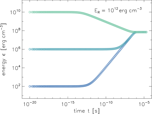
Figure 1: A simple single zone radiation matter coupling test, with $\kappa_{\rm P}=0.4\,\rm cm^{2}\,\rm g^{-1}$, $\bar{\mu}=0.6$, $\gamma=\nicefrac{{5}}{{3}}$, and $\rho=10^{-7}\,\rm g\,\rm cm^{-3}$.

A standard test case for assessing the interplay of the radiation-matter-coupling with the radiation diffusion are radiative shocks, for which there exist semi-analytic solutions in simplified situations [32]. In Fig. 2, we plot the solution of the ${\rm Ma}=2$ case from ref. [32], using $n=128$ grid cells in the $x$ direction, as well as two levels of adaptive mesh refinement (triggered by gradients in the thermal energy, $\epsilon$), which are shown as gray shaded areas in the plot. As seen in the lower panel of Fig. 2, apart from the shock location (which has been shifted by $x_{\rm offs}=22.5\,\rm cm$ with respect to the semi-analytic solution), all quantities agree to within $\permil$ accuracy. We have also successfully performed the harder ${\rm Ma}=5$ test, which we omit here for brevity. An excellent description of the radiative shock test, including the precise values used for initial conditions, can be found in sect. 4.4 of ref. [18].

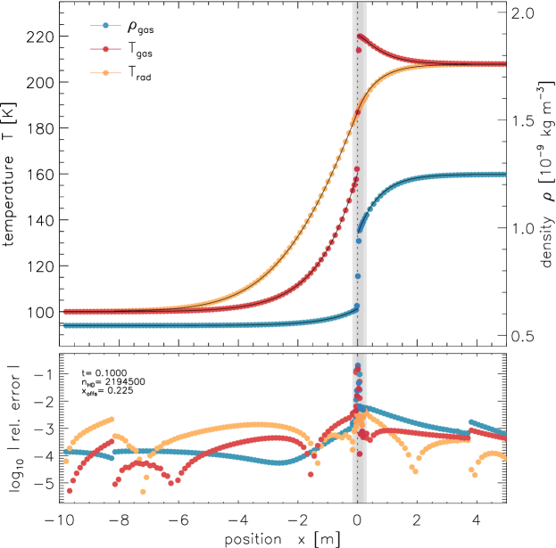
Figure 2: Radiative shock with ${\rm Ma}=2$ and resolution $n=128$ +2 levels of adaptive mesh refinement (shaded areas). Upper panel: Profiles of $\rho_{\rm gas}$ (blue), $T_{\rm gas}$ (red), and $T_{\rm rad}$ (yellow). Lower panel: deviation from the semi-analytic solution (black).

3.2 Preliminary global MHD simulations with irradiation

Returning to the original motivation for implementing radiative physics in our modified version of the nirvana-iii code, we conclude by presenting a preliminary snapshot of a global axisymmetric protoplanetary disk simulation including Ohmic resistivity, ambipolar diffusion, radiation diffusion, and stellar irradiation. The ultimate goal of these simulations is to study how the mass-loading of the magnetocentrifugal wind depends on the disk thermal structure.

Figure 3: Detail from a proof-of-concept global MHD simulation of a PPD with ambipolar diffusion, radiative transfer and stellar irradiation, showing $\bar{B}_{\phi}$ (colour), poloidal velocity (black) and magnetic field lines (white), and iso-contours of the radiation temperature (grey).

As a simple proof-of-concept, we present a close-up of the inner disk in a simulation covering seven (initial) pressure scale heights in latitude (see Fig. 3). The basic disk setup is very similar to the one used in ref. [6], and we have additionally used opacities that correspond to a dust-depletion of a factor of ten compared to the typical interstellar abundance. Similar to our previous simulations, the magnetic field lines (white) bend outward, and in the upper disk layers, where the matter is sufficiently coupled to the magnetic field, a magnetocentrifugal disk wind ensues (black vectors).

Iso-contour lines (gray) of the radiation temperature $T_{\rm rad}\!\equiv\!E_{\rm R}^{\nicefrac{{1}}{{4}}}a_{\rm R}^{\nicefrac{{-1}}{{4}}}$ illustrate the disk’s thermal structure that deviates noticeably from the constant-on-cylinders radial temperature profile $T=T(R)$, that we have assumed previously. The presented preliminary run used a reduced-speed-of-light factor $\phi=10^{-4}$. Further tests will show whether the chosen time-explicit framework is powerful and efficient enough to be of use in realistic situations.

The author thanks Jon Ramsey for many useful discussions, for carefully reading this manuscript, and for providing his code to compute semi-analytic reference solutions of radiative shocks. Dmitry Semenov is acknowledged for providing helpful clues in connection with his opacity code. The research leading to these results has received funding from the European Research Council (ERC) under the European Union’s Horizon 2020 research and innovation programme (grant agreement No 638596).

References

References

- [1] Williams J P and Cieza L A 2011 ARA&A 49 67–117 (Preprint 1103.0556)
- [2] Johansen A, Blum J, Tanaka H, Ormel C, Bizzarro M and Rickman H 2014 PPVI 547
- [3] Gressel O, Nelson R P and Turner N J 2012 MNRAS 422 1140–1159 (Preprint 1202.0771)
- [4] Turner N J, Fromang S, Gammie C, Klahr H, Lesur G, Wardle M and Bai X N 2014 PPVI 411–432
- [5] Bai X N and Stone J M 2013 ApJ 769 76 (Preprint 1301.0318)
- [6] Gressel O, Turner N J, Nelson R P and McNally C P 2015 ApJ 801 84 (Preprint 1501.05431)
- [7] Lesur G, Kunz M W and Fromang S 2014 A&A 566 A56 (Preprint 1402.4133)
- [8] Simon J B, Lesur G, Kunz M W and Armitage P J 2015 MNRAS 454 1117–1131 (Preprint 1508.00904)
- [9] Bai X N, Ye J, Goodman J and Yuan F 2016 ApJ 818 152 (Preprint 1511.06769)
- [10] Bai X N 2016 ApJ 821 80 (Preprint 1603.00484)
- [11] Suzuki T K, Ogihara M, Morbidelli A, Crida A and Guillot T 2016 A&A (Preprint 1609.00437)
- [12] Ziegler U 2004 JCoPh 196 393–416
- [13] Ziegler U 2011 JCoPh 230 1035–1063
- [14] Jiang Y F, Stone J M and Davis S W 2012 ApJS 199 14 (Preprint 1201.2223)
- [15] Levermore C D and Pomraning G C 1981 ApJ 248 321–334
- [16] Bitsch B, Crida A, Morbidelli A, Kley W and Dobbs-Dixon I 2013 A&A 549 A124 (Preprint 1211.6345)
- [17] Kuiper R and Klessen R S 2013 A&A 555 A7 (Preprint 1305.2197)
- [18] Ramsey J P and Dullemond C P 2015 A&A 574 A81 (Preprint 1409.3011)
- [19] Noebauer U, Sim S, Kromer M, Röpke F and Hillebrandt W 2012 MNRAS 425 1430 (Preprint 1206.6263)
- [20] González M, Vaytet N, Commerçon B and Masson J 2015 A&A 578 A12 (Preprint 1504.01894)
- [21] Semenov D, Henning T, Helling C, Ilgner M and Sedlmayr E 2003 A&A 410 611–621
- [22] Gnedin N Y and Abel T 2001 NewA 6 437–455 (Preprint astro-ph/0106278)
- [23] Skinner M A and Ostriker E C 2013 ApJS 206 21 (Preprint 1306.0010)
- [24] Hartmann L 1998 Accretion Processes in Star Formation
- [25] Meyer C D, Balsara D S and Aslam T D 2012 MNRAS 422 2102–2115
- [26] Burchard H, Deleersnijder E and Meister A 2003 AppliedNumMath 47 1 – 30 ISSN 0168-9274
- [27] Nelson R P, Gressel O and Umurhan O M 2013 MNRAS 435 2610–2632 (Preprint 1209.2753)
- [28] Gressel O, Nelson R P, Turner N J and Ziegler U 2013 ApJ 779 59 (Preprint 1309.2871)
- [29] Chiang E I and Goldreich P 1997 ApJ 490 368–376 (Preprint astro-ph/9706042)
- [30] Bruls J H M J, Vollmöller P and Schüssler M 1999 A&A 348 233–248
- [31] Turner N J and Stone J M 2001 ApJS 135 95–107 (Preprint astro-ph/0102145)
- [32] Lowrie R B and Edwards J D 2008 Shock Waves 18 129–143