Monte Carlo radiation hydrodynamics: methods, tests and application to supernova Type Ia ejecta

Abstract

In astrophysical systems, radiation-matter interactions are important in transferring energy and momentum between the radiation field and the surrounding material. This coupling often makes it necessary to consider the role of radiation when modelling the dynamics of astrophysical fluids. During the last few years, there have been rapid developments in the use of Monte Carlo methods for numerical radiative transfer simulations. Here, we present an approach to radiation hydrodynamics that is based on coupling Monte Carlo radiative transfer techniques with finite-volume hydrodynamical methods in an operator-split manner. In particular, we adopt an indivisible packet formalism to discretize the radiation field into an ensemble of Monte Carlo packets and employ volume-based estimators to reconstruct the radiation field characteristics. In this paper the numerical tools of this method are presented and their accuracy is verified in a series of test calculations. Finally, as a practical example, we use our approach to study the influence of the radiation-matter coupling on the homologous expansion phase and the bolometric light curve of Type Ia supernova explosions.

1 Introduction

In studying astrophysical objects, a detailed understanding and description of the radiation field is vital, particularly if synthetic observables are to be computed for comparison with observations. Conceptually, the radiation field in a fluid is not independent of the fluid state and their co-evolution has to be described self-consistently within the framework of radiation hydrodynamics. Depending on the dynamical importance of the radiation field and the strength of the radiation-matter coupling, different strategies can be followed. If the energy associated with the radiation field is negligible compared to the total energy content, a de-coupled approach may be followed. For example, such a method has been used for the determination of synthetic light curves and spectra for Type Ia supernova (SN Ia) explosions around maximum light (e.g. Kasen et al., 2006; Kromer & Sim, 2009; Jack et al., 2011). In cases where the radiative terms are dynamically important, however, a fully de-coupled treatment of the radiation field is not possible. For such applications a variety of different techniques have been used to follow the co-evolution of the radiation-matter state. In optically thick environments, the radiation field is well-described by the diffusion approximation and its evolution in radiation-hydrodynamical simulations can be incorporated by using flux limited diffusion methods (Levermore & Pomraning, 1981). This numerical prescription is used, for example, in the modelling of radiation dominated accretion discs (e.g. Turner et al., 2003; Hirose et al., 2009). In the opposite case of low optical depth, the influence of the radiation field may be treated by including a radiative cooling term (e.g. Townsend, 2009; van Marle & Keppens, 2011), as is often done in studies of stellar winds (e.g. Garcia-Segura et al., 1996; Mellema & Lundqvist, 2002). In the intermediate regimes between the two extremes, a full radiation-hydrodynamical description of the radiation-matter state is necessary, for example when accounting for convective motions in studies of stellar atmospheres (e.g. Stein & Nordlund, 1998; Asplund et al., 2000), shock breakouts in supernovae (e.g. Blinnikov et al., 2000; Höflich & Schaefer, 2009; Piro et al., 2010) or when studying interactions of stellar explosions with circumstellar material (e.g. Fryer et al., 2010; Kasen, 2010).

In this paper we present the numerical methods and the application of a new approach to radiation hydrodynamics that is based on Monte Carlo radiative transfer techniques. A similar strategy has been pursued in the calculations presented in Kasen et al. (2011). Monte Carlo methods have already shown tremendous success in pure radiative transfer applications (e.g. Fleck & Cummings, 1971; Abbott & Lucy, 1985; Mazzali & Lucy, 1993; Long & Knigge, 2002; Carciofi & Bjorkman, 2006; Kasen et al., 2006; Harries, 2011). Within this probabilistic approach, complex radiation-matter interaction physics can be simulated and problems with arbitrary geometries can be addressed. Here we aim to extend the Monte Carlo method to radiation-hydrodynamical calculations and explore its practicality for modern astrophysical applications.

The focus of this paper is to present the theoretical and numerical foundations and to verify the operation of our Monte Carlo radiation-hydrodynamical method. We begin with a brief overview of the theoretical concepts that govern radiating flows in Section 2, which is followed by an extensive description of the numerical methods of our approach in Section 3. The physical accuracy and the computational feasibility of the techniques presented here are assessed in Section 4, in which the results of a series of test calculations are described. As a first application of the method in astrophysical environments we report in Section 5 on our investigation of SNe Ia ejecta. In particular, we study the influence of the radiation-matter coupling on the ejecta structure and the resulting effects on the bolometric light curve during the homologous expansion phase. We summarize our results and conclude in Section 6.

2 Theoretical Background

To model environments in which a significant part of the total energy is stored in the radiation field, one must deal with the coupled evolution of the matter state and the radiation field. The former changes due to external forces, gradients of the thermodynamic variables and the radiation pressure acting on the matter. Such radiation pressure gradients are the consequence of anisotropies in the radiation field whose temporal evolution is driven by its interactions with the surrounding medium. Generally, these interactions are strongly dependent on the state of matter, i.e. on its density, temperature and composition. The theory of radiating fluids provides an adequate self-consistent description of the dynamical behaviour of the radiation-hydrodynamical state of the coupled radiation field-matter system. In the following section, we will give a brief outline of some important aspects of this theory. In-depth discussions can be found in standard textbooks, e.g. Mihalas & Mihalas (1984).

To describe the energy and the momentum of radiating fluids, the standard hydrodynamical equations expressing conservation of momentum and energy are extended by including additional source terms that account for the influence of the radiation field. In astrophysical environments, the physical viscosity is typically insignificant compared to the viscosity inherent to the numerical schemes used to model fluid flows. Consequently, the ideal Euler equations are commonly employed. Modified by the influence of the radiation field, these take the form

$$\rho\frac{\mathrm{D}}{\mathrm{D}t}\mn@boldsymbol{u}=\mn@boldsymbol{f}-\nabla P+\mn@boldsymbol{G},$$ (1)

$$\rho\frac{\mathrm{D}}{\mathrm{D}t}e=\mn@boldsymbol{u}\cdot\mn@boldsymbol{f}-\nabla\cdot(P\mn@boldsymbol{u})+cG^{0}.$$ (2)

Mass conservation, expressed by the continuity equation

$$\frac{\mathrm{D}}{\mathrm{D}t}\rho+\rho(\nabla\cdot\mn@boldsymbol{u})=0,$$ (3)

is not affected by the radiation field. Here, $\rho$, $\mn@boldsymbol{u}$, $e$ and $P$ denote the fluid density, velocity, total energy and thermodynamic pressure, respectively. Possible external forces are accounted for by the force density $\mn@boldsymbol{f}$. The radiation field acts as an additional energy and momentum source in the form of the radiation 4-force components $G^{0}$ and $\mn@boldsymbol{G}$ (see below). Note that we have formulated the equations in terms of substantial derivatives

$$\frac{\mathrm{D}}{\mathrm{D}t}=\frac{\partial}{\partial t}+\mn@boldsymbol{u}\cdot\nabla,$$ (4)

which capture changes in the co-moving fluid frame.

The $G$-terms essentially describe momentum and energy flows caused by an imbalance of absorption and emission interactions between the radiation field and its surrounding medium. Quantitatively, these interactions are characterised by the opacity, $\chi(\mn@boldsymbol{x},t;\mn@boldsymbol{n},\nu)$, and the emissivity $\eta(\mn@boldsymbol{x},t;\mn@boldsymbol{n},\nu)$ of the medium. These material functions depend on the frequency ($\nu$) and the propagation direction ($\mn@boldsymbol{n}$) of the radiation and will in general vary with time ($t$) and position ($\mn@boldsymbol{x}$), since the radiation-matter interactions depend strongly on the fluid state. The radiation force components can be specified in terms of these material functions and the specific intensity, $I(\mn@boldsymbol{x},t;\mn@boldsymbol{n},\nu)$:

$$G^{0}=\frac{1}{c}\int_{0}^{\infty}\mathrm{d}\nu\int\mathrm{d}\Omega~{}[\chi(\mn@boldsymbol{x},t;\mn@boldsymbol{n},\nu)I(\mn@boldsymbol{x},t;\mn@boldsymbol{n},\nu)-\eta(\mn@boldsymbol{x},t;\mn@boldsymbol{n},\nu],$$ (5)

$$G^{i}=\frac{1}{c}\int_{0}^{\infty}\mathrm{d}\nu\int\mathrm{d}\Omega~{}n^{i}\left[\chi(\mn@boldsymbol{x},t;\mn@boldsymbol{n},\nu)I(\mn@boldsymbol{x},t;\mn@boldsymbol{n},\nu)-\eta(\mn@boldsymbol{x},t;\mn@boldsymbol{n},\nu)\right].$$ (6)

These can be understood as the net absorbed or emitted energy and momentum, respectively. The temporal evolution of the radiation field itself is in turn driven by the interaction with the environment

$$\left(\frac{1}{c}\frac{\partial}{\partial t}+\mn@boldsymbol{n}\cdot\nabla\right)I(\mn@boldsymbol{x},t;\mn@boldsymbol{n},\nu)=$$

$$\qquad\eta(\mn@boldsymbol{x},t;\mn@boldsymbol{n},\nu)-\chi(\mn@boldsymbol{x},t;\mn@boldsymbol{n},\nu)I(\mn@boldsymbol{x},t;\mn@boldsymbol{n},\nu).$$ (7)

The combination of Equations (1), (2), (3), (7) and an equation of state, relating thermodynamic pressure with internal energy, provides the full set of radiation-hydrodynamical equations that describe a radiating fluid. In this formulation, Equations (5) and (6) describe how the energy and momentum transfer is obtained from the temporal evolution of the radiation field. In the following, we present in detail the numerical approach we developed to solve the radiation-hydrodynamical problem formulated by this set of equations.

3 Numerical Methods

To determine the state of a radiating fluid, Equations (1), (2), (3), (7) and the equation of state have to be solved simultaneously. Key to our approach is the application of a simple operator splitting scheme (see e.g. LeVeque, 2002, for a detailed description of the operator splitting technique). In this Godunov-splitting framework, the temporal evolution is determined progressively, accounting for the pure hydrodynamical effects and the influence of the radiation field independently and in sequence. Specifically, in each time step, a new radiation hydrodynamical state is found by first performing a fluid dynamical calculation neglecting all radiative influences. For this step we employ a finite-volume hydrodynamical scheme, namely the piecewise parabolic method (PPM, Colella & Woodward, 1984). This is followed by a second step which only accounts for the influence of the terms in the equations governing the evolution of the radiation field and the fluid-dynamics terms are neglected. For this part of the simulation, we carry out time-dependent Monte Carlo radiative transfer calculations, which allow us to evaluate the radiation terms and use them to update the hydrodynamical state.

The following sub-sections describe our scheme and the involved computational methods. We begin with an outline of the hydrodynamics solver in Section 3.1, followed by a detailed presentation of the Monte Carlo radiative transfer techniques in Sections 3.2 to 3.11. The final step of updating the fluid state to account for the influence of the radiation field is described in Section 3.12.

3.1 Hydrodynamical Calculation

The hydrodynamical sub-problem of the operator-split approach is solved with the piecewise parabolic method of Colella & Woodward (1984). This higher-order Godunov scheme is based on reconstructing a continuous fluid state from a discrete representation on a computational grid by a series of parabolas. In the spirit of finite-volume approaches, Riemann problems are defined at the cell interfaces by discontinuities in the fluid properties, which arise from integrating the reconstructed fluid state over the domains of dependence, i.e. the regions that can influence the interfaces. The solutions to the Riemann problems determine the flux through the interfaces. By balancing the resulting in- and outflows in the grid cells, the temporal evolution of the fluid state can be calculated for one time step. This second-order reconstruction scheme provides higher accuracy over the traditional constant-reconstruction method of Godunov (1959). The detailed implementation of PPM in our radiation hydrodynamics code follows Edelmann (2010). After determining the new fluid state, a Monte Carlo simulation is started to address the evolution of the radiation field as the second half of the splitting scheme.

3.2 Monte Carlo Techniques

In our Monte Carlo approach the radiation field is discretized into a large number of Monte Carlo quanta, hereafter referred to as packets. Each of them carries a fraction of the radiation field energy and is propagated through the medium. The propagation path is determined stochastically but in accordance with the transfer equation (7). From the ensemble of packet trajectories, all relevant radiation field quantities can be reconstructed.

With the increasing availability of computational resources, Monte Carlo techniques have become a very popular and rewarding approach to radiative transfer problems. Among the numerous applications of Monte Carlo radiative transfer techniques in astrophysics are the calculation of mass-loss rates in hot star winds (see e.g. Abbott & Lucy, 1985; Lucy & Abbott, 1993; Vink et al., 2000; Sundqvist et al., 2010), light curves and spectra of SNe Ia (see e.g. Mazzali & Lucy, 1993; Lucy, 2005; Kasen et al., 2006; Sim, 2007; Kromer & Sim, 2009), ionization structure and synthetic spectra of photoionized nebulae (e.g. Ercolano et al., 2003), mass-outflows in cataclysmic variables (e.g. Long & Knigge, 2002; Noebauer et al., 2010) or active galactic nuclei (e.g. Sim, 2005). Compared with classical ray-tracing techniques, the Monte Carlo approach has certain advantages. Most important, from a physical viewpoint, is the ease with which complex scattering and absorption processes can be incorporated. Since all interactions with the surrounding medium can be directly simulated during the propagation of the Monte Carlo packets, even the most complex atomic processes can be included in the radiative transfer calculation (see e.g. Lucy, 2002, 2003, 2005). These interactions are all simulated locally in the co-moving frame, making the Monte Carlo algorithm entirely independent of the large-scale properties of the simulation and readily applicable even to problems with arbitrarily complex multi-dimensional geometries.

Apart from these physically motivated advantages, the Monte Carlo method also brings computational benefits. As the propagation of one packet is independent of the behaviour of all others, Monte Carlo radiative transfer calculations can be easily parallelised and scale very well to large numbers of computational cores. This is of great significance since the efficient use of high performance computing facilities is an important consideration for the feasibility of modelling complex astrophysical systems.

Of course, Monte Carlo radiative transfer methods also have their drawbacks. The accuracy and computational efficiency of the Monte Carlo approach are limited by the number of packets that discretize the radiation field and by the number of physical interactions they simulate. Consequently, whether Monte Carlo radiative transfer methods are appropriate strongly depends on the specific problem under consideration (e.g. Pincus & Evans, 2009). For example, in some applications, a detailed radiative transfer treatment is not required and the dynamical behaviour of the radiation field can be adequately addressed with approximate methods which perform faster than the Monte Carlo approach (e.g. Kuiper et al., 2010). Independently of the specific application, Monte Carlo methods always introduce a certain level of statistical fluctuations in the simulations. We shall return to the subject of minimising the influence of this Monte Carlo noise in Sections 3.10 and 3.11.

3.3 Discretization

As mentioned above, in the Monte Carlo approach the radiation field is discretized into packets. In early uses of the Monte Carlo machinery, e.g. in Avery & House (1968), the number of photons described by a packet was held constant throughout the simulation. However, we follow Abbott & Lucy (1985) and instead choose to discretize into packets of constant radiative energy. At every instant in the simulation, each packet represents a monochromatic parcel of radiative energy – i.e. a number of identical photons, all with a certain frequency $\nu$. When packets interact with the fluid, both the number of photons and the photon frequency associated with a packet can change but the energy it carries in the local rest frame of the fluid remains fixed. In addition, the energy packets are indivisible – i.e. processes may create or destroy packets but never cause them to be split into multiple packets (see Lucy, 2002, 2003, 2005). This approach is motivated by the fact that total energy is conserved in interactions between the radiation field and its surrounding medium but the number of photons generally is not. The indivisible energy-packet method has been shown to be extremely powerful in solving radiative equilibrium problems owing to the ease with which it can ensure energy conservation (see e.g. Lucy, 1999). By extending the method to include a net energy exchange between the radiation field and the matter, we continue to exploit the efficiency of this approach together with the properties of PPM to ensure global energy conservation in our simulations. The use of indivisible packets also avoids computational difficulties arising in cases where a fixed photon-number approach would require that packets are split (e.g. in modelling fluorescence or recombination cascades, where a physical process excited by a single photon leads to the re-emission of many). With the indivisible packet method, these processes are simulated with a probabilistic approach such that no packet splitting is required but that all the cascade channels are correctly sampled when a sufficiently large number of Monte Carlo packets are included (see Lucy, 2002).

With this discretization scheme, the Monte Carlo packets are naturally well-suited to represent the mean intensity of the radiation field and its temporal evolution. In addition, all derived radiation field characteristics can be easily formulated and reconstructed from Monte Carlo estimators and fully frequency-dependent opacities could be readily implemented. However, the radiative flux is in general less accurately captured by the ensemble of energy packets. We will discuss the implication of this in more detail when considering statistical noise and the accurarcy of our approach in Section 3.11.

3.4 Reference Frames

An accurate and detailed description of the dynamical behaviour of the radiation field requires that special relativistic effects are considered. We have therefore designed our Monte Carlo radiative transfer algorithm to account for at least all first order special relativistic effects. In principle, there are no obstacles to extending the method to higher order corrections.

For handling relativistic effects, we must clearly distinguish between two reference frames. We define the spatial and temporal discretization of the problem (i.e. our numerical grid) in the “lab” (or “observer”) frame. The initialisation and propagation of the Monte Carlo packets is also performed in that frame. However, the natural choice for the treatment of matter-radiation interactions is the local rest frame of the fluid, which we will refer to as the “co-moving” frame. Henceforth, a subscript 0 will be used to identify quantities that are defined in the local co-moving frame.

3.5 Simplifications Adopted

For the sake of clarity, in this section and below, we adopt some simplifications that apply to our current implementation and the test problems that we address in Sections 4 and 5. In particular, we restrict ourselves to one-dimensional problems, e.g. plane-parallel or spherically-symmetric media. By arranging the problem setup such that the symmetry axis coincides with the coordinate $z$-axis the radiation propagation direction can be specified by the scalar

$$\mu=\mn@boldsymbol{n}\cdot\mn@boldsymbol{e}_{z}.$$ (8)

In spherically symmetric geometries, $\mu$ is measured with respect to the radial direction. As a consequence of the symmetry properties of the problems we consider, all radiation-hydrodynamical quantities only vary along one spatial coordinate. Thus, the components of the radiation force in the other two orthogonal directions ($G^{1}$ and $G^{2}$) vanish and will not be considered further.

In addition to the geometry restrictions, we treat radiative transfer in a grey, i.e. frequency-independent, approximation. Scattering interactions between the radiation field and the surrounding material are assumed to be coherent and isotropic. We stress, however, that all these simplifications are not necessary – the approach can be readily generalized to multiple dimensions and frequency-dependent opacities. Finally, we use an ideal gas equation of state to relate fluid internal energy and thermodynamic pressure.

3.6 Packet Initialisation

At the beginning of a simulation, we need to generate an initial population of Monte Carlo packets that describe the initial radiation field. This generation process includes assigning each packet an initial position, direction and frequency. All the steps involved in this process have to accommodate the probabilistic nature of the Monte Carlo machinery.

To initialize the population of Monte Carlo packets, an initial condition for the radiation field has to be chosen. As an illustrative example, we assume that the simulation is to be initialized in local thermodynamic equilibrium (LTE). In this case, the radiation energy density in the co-moving frame, $E_{0}$, follows the Stefan-Boltzmann law

$$E_{0}=a_{\mathrm{R}}T^{4}.$$ (9)

To correctly initialize the Monte Carlo packets, the total energy is first transformed into the lab-frame and summed over the entire computational domain

$$\mathcal{E}_{\mathrm{tot}}=\sum_{i}\gamma^{2}\left(1+\frac{1}{3}\beta^{2}\right)a_{\mathrm{R}}T_{i}^{4}\Delta V_{i}.$$ (10)

Here, $\beta$ and $\gamma$ denote the usual parameters of special relativity

$$\beta=\frac{u}{c},$$ (11)

$$\gamma=\frac{1}{\sqrt{1-\beta^{2}}},$$ (12)

and the index $i$ runs over all grid cells. The total energy $\mathcal{E}_{\mathrm{tot}}$ is then divided equally into a chosen number of Monte Carlo packets (all packets are assigned the same initial lab-frame energy), which are spread over the grid cells according to the local radiative energy content. The initial position of a packet within a grid cell is chosen randomly. In LTE, the radiation field is isotropic in the co-moving frame, i.e. it has no angular dependence. Due to angle aberration effects, this isotropy is lost during the transformation into the lab frame. Consequently, the assignment of the initial propagation direction has to account for the angular dependence of the radiation field in the lab frame. In the grey approximation and under the restriction to one-dimensional problems, the LTE lab frame specific intensity follows

$$I(\mu)=\frac{B(T)}{\gamma^{4}(1-\beta\mu)^{4}},$$ (13)

with $B(T)$ denoting the frequency-integrated Planck function

$$B(T)=\frac{\sigma_{\mathrm{R}}}{\pi}T^{4}.$$ (14)

This angular dependence can be translated into a probability density

$$\rho(\mu)=\frac{(1-\beta^{2})^{3}}{2(1+1/3\beta^{2})}\frac{1}{(1-\beta\mu)^{4}},$$ (15)

which can be sampled to give the relativistically correct directional distribution of the initial Monte Carlo packets. In the classical limit ($\beta\rightarrow 0$, $\gamma\rightarrow 1$), the density simplifies to

$$\rho(\mu)=\frac{1}{2},$$ (16)

which can be easily sampled by the random number experiment

$$\mu=2\xi-1,$$ (17)

where $\xi$ denotes a random number drawn uniformly from the interval $[0,1]$. In the more general case, Equation (15) must be sampled, leading to a more complex expression for $\mu$ in terms of $\xi$, but the same principle applies.

In general, each packet also has to be assigned a photon frequency ensuring that the packets represent the correct spectrum of the radiation field. In this work, however, this step can be skipped since we currently adopt a grey-approximation. A possible realisation of the more general sampling process can be found in Lucy (1999).

3.7 Sequence of Monte Carlo simulations

After their initialization at the beginning of the simulation, the Monte Carlo packets are propagated through the medium. During each time step, the packets are able to move (see Section 3.8), some packets are destroyed and others are created (see Section 3.9). At the end of each time step, the properties of the currently active packets are stored so that these packets can be reactivated at the start of the next time step, after the fluid properties have been updated (see Section 3.12). A graphical outline of the program flow is shown in Fig. 1.

Figure 1: Flow chart of the operator split algorithm and a detailed outline of the Monte Carlo radiative transfer step. During this process, the trajectories of all packets are determined and the radiation field characteristics are calculated by the Monte Carlo estimators.

3.8 Packet Propagation

In the Monte Carlo simulation, the packets propagate with the speed of light $c$ through the medium. To simulate the dynamical evolution of the radiation field, the packets undergo interactions with the surrounding material as they propagate. In the Monte Carlo method, the propagation and interactions are treated stochastically. In particular, the location of packet interactions are determined by random number experiments – the trajectory of a propagating packet is terminated by an interaction with the surrounding medium when it covered a path-length

$$l=-\frac{\ln\xi}{\chi},$$ (18)

which follows from sampling the extinction law

$$I=I_{0}\mathrm{e}^{-l\chi}.$$ (19)

In addition to simulating physical interactions in this stochastic manner, two additional events that stem from the spatial and temporal discretization have to be taken into account. During the propagation process, packets can cross grid cell boundaries or reach the end of the current simulation time step. In the case of cell crossings, the changing fluid properties have to be taken into account, i.e. the interaction length $l$ has to be recalculated. Since the Monte Carlo packets propagate with the speed of light, they will at maximum travel a distance of $d=c\Delta t$ during a simulation cycle of duration $\Delta t$. At this point the propagation of a packet is suspended and its properties are stored in order to resume the propagation at the beginning of the next time step.

3.9 Interaction Formalism

Since our Monte Carlo packets represent photon packets, their interactions should model the physical interactions of photons with the surrounding medium: scattering, absorption and emission processes. When a packet experiences a physical interaction (i.e. once it has propagated the path-length given by Equation 18), we must first determine the nature of the interaction. If we include both scattering ($\sigma$) and absorption ($\kappa$) contributions to the opacity

$$\chi=\sigma+\kappa,$$ (20)

the relative strength of these will determine the probability of the interaction having been a scattering or absorption event. In particular, we identify that a packet scatters if

$$\xi\leq\frac{\sigma}{\sigma+\kappa}$$ (21)

is fulfilled. To treat a coherent scattering event, the packet is transformed into the co-moving frame

$$\varepsilon_{0}=\varepsilon\gamma(1-\beta\mu)$$ (22)

where the packet energy is conserved and a new propagation direction $\mu_{0}^{\prime}$ is drawn isotropically (cf. Equation 17). Afterwards, the packet properties are transformed back into the lab frame

$$\varepsilon^{\prime}=\varepsilon_{0}\gamma(1+\beta\mu_{0}^{\prime}),$$ (23)

$$\mu^{\prime}=\frac{\mu_{0}^{\prime}+\beta}{1+\beta\mu_{0}^{\prime}},$$ (24)

to resume the propagation. For all other outcomes of the experiment (Equation 21), an absorption event occurs, resulting in the destruction of the packet. Consequently, this packet stops its propagation and is no longer considered in the remaining simulation process.

Destruction of packets by absorption interactions drains the energy content of the radiation field. However, radiation energy is also created due to emission by the medium. In the case of thermal emission, the radiative energy pool in a grid cell of volume $\Delta V$ is increased by

$$\Delta\mathcal{E}=4\gamma\kappa\sigma_{\mathrm{R}}T^{4}\Delta V\Delta t$$ (25)

during a time step of size $\Delta t$ assuming constant temperature and opacity. To represent this effect in the Monte Carlo calculation, a number of new packets are created and launched during each cycle whose total energy is consistent with this energy injection. The initial packet properties (e.g. direction of propagation, which we assume to be isotropic in the co-moving frame) are assigned by sampling appropriate probability distributions, in analogy to the process of representing the initial radiation field at the onset of the simulation (see Section 3.6). However, these emitted packets are not all injected into the simulation at the start of a time step but at randomly determined times during the time step, thereby accounting for the continuous energy injection by the thermal emission process.

In all interaction processes, momentum and/or energy are transferred between the radiation field and the surrounding material. Through their interaction behaviour, the packets account directly for the impact of the momentum and energy flows on the radiation field. The complementing effect on the surrounding fluid material is equally important (see Equations 1 and 2). These flow terms can be reconstructed from the Monte Carlo simulation with the help of volume-based Monte Carlo estimators (see next Section, 3.10).

3.10 Monte Carlo Estimators

The Monte Carlo packets were introduced to discretize the radiation field and, during their propagation, simulate its interactions with the medium. In principle, all properties of the radiation field can be directly determined from the instantaneous properties of the packets at any given time, e.g. from their instantaneous distribution in real space, momentum space and frequency space at the end of a time step. However, the accuracy with which radiation quantities can be reconstructed is limited by Monte Carlo noise and it is advantageous to consider how to extract maximum information from the Monte Carlo simulation. Lucy (1999) showed that radiation field quantities can be more accurately determined by using volume-based Monte Carlo estimators rather than directly counting properties of the packets. In this approach, the complete ensemble of trajectories that packets traverse during a time step is used to reconstruct the radiation field characteristics (see Lucy, 1999, 2003, 2005). Thus, each packet contributes to the cell-averaged values of the radiation field characteristics according to the fraction of the time that it spent in the cell. Compared to reconstruction methods based on considering the final packet distribution at the end of the propagation step, this cumulative approach significantly reduces the Monte Carlo noise, which is in general the limiting factor in the applicability of Monte Carlo methods. To reconstruct the cell-averaged radiation field energy density all packet trajectory segments that cross the cell under consideration or lie within it are taken into account. On each of these trajectory segments, the packet contribution scales with its energy $\varepsilon$. Every contribution is weighted according to the ratio of the time $\delta t_{i}$ the packet spent on the trajectory element to the full duration of the simulation time step $\Delta t$. Replacing the propagation time with the path length $l_{i}=c\delta t_{i}$ of the individual segments and summing up, gives the estimator

$$E=\frac{1}{\Delta Vc\Delta t}\sum_{i}\varepsilon l_{i}$$ (26)

for the radiation field energy density. Here, the summation runs over all trajectory elements in one cell, implying that a packet may contribute several times to the estimator. Using the fundamental relation between the radiation field energy density and the mean intensity

$$J=\frac{c}{4\pi}E,$$ (27)

a Monte Carlo estimator for the latter can be formulated (see Lucy, 1999, equation 12)

$$J=\frac{1}{4\pi\Delta V\Delta t}\sum\varepsilon l.$$ (28)

By restricting the estimator sum to contributions by packets propagating into a certain directional bin $[\mu,\mu+\Delta\mu]$,

$$I(\mu)\Delta\mu=\frac{1}{2\pi\Delta V\Delta t}\sum_{[\mu,\mu+\Delta\mu]}\varepsilon l.$$ (29)

the specific intensity can also be determined in a similar manner (see Lucy, 2005, equation 2). With this expression, estimators for all radiation field characteristics that depend on the specific intensity or its moments can be easily formulated.

For radiation-hydrodynamical problems, the radiation force components have to be reconstructed from the Monte Carlo simulation to determine the energy and momentum flow between the fluid and radiation field. The components of the radiation force can be interpreted as the difference between absorbed and emitted radiation energy and momentum respectively. We clearly separate the contributions to the radiation force terms caused by scattering interactions from the energy and the momentum transferred in pure absorption and emission events. To identify the latter contribution, each packet trajectory is considered to affect the cell-averaged absorbed energy, even if the packet did not explicitly interact during the propagation cycle. Conceptually, we are therefore counting all absorption events that could have happened in the simulation (weighted by their probability of occurring), rather than simply counting the events that did happen. Thus, while propagating a path-length $l$, a packet contributes with

$$\Delta E=\frac{l\kappa\varepsilon}{\Delta V}$$ (30)

and with

$$\Delta p=\frac{\mu l\kappa\varepsilon}{c\Delta V}$$ (31)

to the cell-averaged absorbed energy and momentum densities respectively. The complementing energy and momentum injection due to thermal emission is determined analytically for each cell. Accounting for the frame transformation into the lab frame the injection rates can be formulated as

$$\dot{E}=4\gamma\kappa\sigma_{\mathrm{R}}T^{4},$$ (32)

$$\dot{p}=\frac{4}{c}\beta\gamma\kappa\sigma_{\mathrm{R}}T^{4}.$$ (33)

In addition to determining the contribution of pure absorption and re-emission events to the energy and momentum transfer terms, scattering interactions have to be incorporated. We consider scattering interactions formally as a combination of an absorption event, followed immediately by the coherent and isotropic re-emission of a Monte Carlo packet. This interpretation allows us to reconstruct the scattering contribution analogously to Equations (30) and (31). In general, however, formulating an analytic expression to quantify the re-emission part is non-trivial. This difficulty can be circumvented by exploiting the fact that Monte Carlo packets are not destroyed in scattering interactions. Thus, the packets can simulate both the absorption and re-emission parts of the scattering events at the same time. By additionally assigning each packet a set of hypothetical “post-scatter” properties, i.e. drawing a propagation direction $\mu_{0}^{\prime}$ that translates into an energy $\varepsilon^{\prime}$ and a direction $\mu^{\prime}$ in the lab frame according to the transformation rules (23) and (24), each packet trajectory $l$ contributes to cell averaged energy and momentum transfer according to

$$\Delta E=\frac{\sigma l}{\Delta V}(\varepsilon^{i}-\varepsilon^{f}),$$ (34)

$$\Delta p=\frac{\sigma l}{c\Delta V}(\mu^{i}\varepsilon^{i}-\mu^{f}\varepsilon^{f}).$$ (35)

Here, the superscripts $i$ and $f$ denote the current packet properties during the propagation and the formal post-scattering state, respectively.

Finally, volume-based Monte Carlo estimators for the radiative force terms $G^{0}$ and $G^{3}$ are obtained by gathering all contributions of scattering and pure absorption/emission events

$$G^{0}=\frac{1}{\Delta Vc\Delta t}\sum l(\chi\varepsilon^{i}-\sigma\varepsilon^{f})-\frac{4}{c}\gamma\kappa\sigma_{\mathrm{R}}T^{4},$$ (36)

$$G^{3}=\frac{1}{\Delta Vc\Delta t}\sum l(\chi\mu^{i}\varepsilon^{i}-\sigma\mu^{f}\varepsilon^{f})-\frac{4}{c}\beta\gamma\kappa\sigma_{\mathrm{R}}T^{4}.$$ (37)

Once transformed into the local co-moving frame, these estimators take the expected form for the corresponding radiation field characteristics measured in this frame. In particular, the estimators (36) and (37) become

$$G^{0}_{0}=\frac{1}{\Delta V_{0}c\Delta t_{0}}\sum\kappa_{0}l_{0}\varepsilon_{0}-\frac{4\pi}{c}\kappa_{0}B(T),$$ (38)

$$G^{3}_{0}=\frac{1}{\Delta V_{0}c\Delta t_{0}}\sum\chi_{0}l_{0}\mu_{0}\varepsilon_{0},$$ (39)

after transformation into the local co-moving frame using

$$G^{0}_{0}=\gamma(G^{0}-\beta G^{3}),$$ (40)

$$G^{3}_{0}=\gamma(G^{3}-\beta G^{0}).$$ (41)

These co-moving frame estimators for $G^{0}_{0}$ and $G^{3}_{0}$ reproduce exactly the radiative energy and momentum sources in this frame, which can be formulated as

$$G^{0}_{0}=\frac{4\pi}{c}\kappa_{0}(J_{0}-B(T)),$$ (42)

$$G^{3}_{0}=\frac{\chi_{0}}{c}F_{0}.$$ (43)

To obtain the same transformation behaviour for the Monte Carlo estimators in spherically-symmetric geometries, the direction scalar has to be averaged over the trajectory segment.

3.11 Monte Carlo Noise

Due to the stochastic nature of the Monte Carlo technique, all associated quantities are subject to statistical fluctuations, limiting the accuracy of the radiative transfer calculation. The obvious approach to reduce the Monte Carlo noise by increasing the number of active packets is limited by computational efficiency considerations. In this context, the concept of volume-based Monte Carlo estimators, as described in the previous section is vital since it allows us to extract the maximum amount of information from the propagation behaviour of a given number of radiation packets. The reduction of the statistical fluctuations in the reconstructed quantities is significant but still limited. In particular, the noise level in the energy-momentum transfer and thus the accuracy with which the radiation-hydrodynamical coupling is captured, varies with the state of the radiation field, due to our discretization scheme and to the form of the radiation force components in the co-moving frame. Reconstructing the energy transfer from a difference of two terms as in Equation (42), yields accurate results if the contributions are clearly separable. However, if the mean intensity deviates from the equilibrium configuration (i.e. $B(T)$) only on the level of the Monte Carlo noise, the resulting heating/cooling term will be obscured by statistical fluctuations. Similarly, the momentum transfer is only accurately captured if the radiative flux is well-resolved (cf. Equation 43). To achieve high accuracy in the reconstruction via the estimator formalism, the packet contributions to the estimators have to be much smaller than the reconstructed quantity. This is the case for the mean intensity, since our discretization scheme (indivisible energy packets) is most naturally suited to well-represent this radiation field characteristic. In the reconstruction of the radiative flux, however, the packet contributions to the estimator are weighted with the propagation direction. As a consequence, the radiative flux is only well-resolved in our approach if $F_{0}\lesssim 4\pi J_{0}$, but obscured by Monte Carlo noise for $F_{0}\ll 4\pi J_{0}$, i.e. for nearly isotropic radiation field configurations.

In summary, our Monte Carlo approach is ideal for describing the mean intensity and our estimators will accurately capture the radiation forces when significant deviations from LTE or from isotropy are present. However, in cases where the radiation field is nearly isotropic or close to the LTE configuration, the radiation hydrodynamical effects, as described in the radiation force terms, may be subject to significant statistical fluctuations. In order to achieve a further suppression of the noise in this regime, we have found it useful to smooth the reconstructed radiation field quantities over neighbouring grid cells. This additional noise reduction method will be of importance when addressing SN Ia ejecta (see Section 5.3).

3.12 Dynamical Influence of the Radiation Field

With the numerical methods described in the previous sections, the temporal evolution of the radiation field is determined in a Monte Carlo step as part of the operator splitting approach to radiation hydrodynamics. After solving the fluid dynamical evolution using PPM and simulating the radiative transfer in the Monte Carlo simulation, the calculation of the new radiation-hydrodynamical state ends with the inclusion of the radiative influence on the dynamics specified by $G^{0}$ and $G^{3}$. These terms are reconstructed from the Monte Carlo simulation using the estimators defined in Equations (36) and (37) and describe the energy and momentum transfer onto the surrounding material. Consequently the fluid energy and momentum are updated according to

$$\rho\frac{\partial}{\partial t}u=G^{3},$$ (44)

$$\rho\frac{\partial}{\partial t}e=cG^{0},$$ (45)

as the second and last step of the Godunov splitting approach. This concludes the calculation of one time step and a new simulation cycle is entered by stepping through the segments of the splitting scheme again, starting by solving the fluid dynamics for the next time step (see Fig. 1).

4 Testing

The methods described in the previous section have been implemented into a numerical code, hereafter referred to as mcrh. Currently, the program is able to calculate the temporal evolution of radiating fluids in an Eulerian or Lagrangian reference frame, assuming grey radiative transfer and one-dimensional geometries (see Section 3.5). Before using the code to model radiative flows in astrophysical environments or implementing more complex geometries and opacities, the computational feasibility and physical accuracy of our approach and its implementation has to be verified. PPM is commonly used to simulate fluid flows in astrophysical applications, e.g. in Type Ia and II supernova explosions (e.g. Röpke & Hillebrandt, 2005; Janka & Mueller, 1996) or in relativistic jets (e.g. Marti et al., 1997) and has already been tested extensively. Consequently, the main focus of this discussion lies in testing the radiative transfer and the radiation-matter coupling components of our approach.

We start this verification process by first testing the propagation behaviour of the Monte Carlo packets. In the next stage, the interaction mechanism is checked by examining the equilibration behaviour in a series of toy simulations. Finally, we turn towards radiative shocks, the standard test problem for radiation hydrodynamics. In calculating sub- and supercritical shocks, the workings of both the radiation-matter coupling and our complete radiation hydrodynamics method can be verified.

4.1 Random Walk

As presented in Section 3.8, the Monte Carlo packets undergo a multitude of physical interactions and numerical events on their propagation trajectories. Since this behaviour is essential for accurately simulating the temporal evolution of the radiation field, our first test calculation aims to verify the packet propagation process. For this purpose, we follow Harries (2011) and consider a purely scattering medium in the optically thick limit. The entire radiation field energy is initially concentrated in the central cell of the computational domain (which has length $L$), mimicking a $\delta$-function. In this problem, the initial radiation peak disperses according to the diffusion equation

$$\frac{\mathrm{d}E}{\mathrm{d}t}=-D\frac{\mathrm{d}^{2}E}{\mathrm{d}z^{2}},$$ (46)

yielding

$$E(z,t)=E(t_{0})\frac{L}{\sqrt{4\pi Dt}}\exp\left(-\frac{z^{2}}{4Dt}\right).$$ (47)

With interactions restricted to scattering only, the diffusion coefficient is given by

$$D=\frac{c}{3\sigma}.$$ (48)

In a Monte Carlo simulation of this problem, the packets are expected to perform a random walk due to the large scattering optical depth. Consequently, the temporal evolution of the radiative energy constitutes a suitable test to verify the correct propagation behaviour of the Monte Carlo packets.

Following Harries (2011), the test simulation is performed in a planar symmetric box of length $L=1\,\mathrm{cm}$ that is divided into 101 equally spaced cells. In the central cell, an initial radiation field energy density of $E=10^{10}\,\mathrm{erg}\,\mathrm{cm^{-3}}$ is deposited and discretized by $10^{5}$ Monte Carlo packets. Fig. 2 shows the temporal evolution of the radiative energy density in our Monte Carlo simulation. The results are compared with the theoretically expected behaviour set by Equation (47). The excellent agreement between the simulation and the theoretical predictions demonstrates the accurate operation of the basic Monte Carlo processes driving the packet propagation.

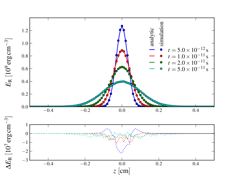
Figure 2: Comparison between the theoretically expected diffusion behaviour (solid lines) of a centrally peaked radiation field in an optically thick, pure scattering medium and the corresponding Monte Carlo simulation (circles). The lower panel shows the absolute difference between the theoretocally expected ($E_{\mathrm{th}}$) and simulated ($E_{\mathrm{sim}}$) energy densities, $\Delta E_{\mathrm{R}}=E_{\mathrm{th}}-E_{\mathrm{sim}}$.

4.2 Equilibration Behaviour

Equally important as the correct propagation behaviour is the accurate calculation of the momentum and energy transfer between the radiation field and the surrounding material. We verify this part of our scheme by examining the relaxation behaviour towards equilibrium in a series of toy simulations. Following Turner & Stone (2001) and Harries (2011), we consider a radiating fluid initially far from equilibrium. In these particular tests, only absorption and thermal emission events occur in the medium and all influences of the thermodynamic and radiation pressure can be neglected. Therefore, the dynamical behaviour of the radiating fluid can be expressed in terms of the radiation field energy density $E_{\mathrm{R}}$ and the internal energy density $E_{\mathrm{G}}$, which follow (see Harries, 2011, equation 23)

$$\frac{\partial}{\partial t}E_{\mathrm{G}}=c\kappa E_{\mathrm{R}}-4\kappa\sigma_{\mathrm{R}}T_{\mathrm{G}}^{4}(E_{\mathrm{G}})$$ (49)

and

$$\frac{\partial}{\partial t}E_{\mathrm{R}}=-\frac{\partial}{\partial t}E_{\mathrm{G}}.$$ (50)

As a first test, we follow the relaxation behaviour of the radiation field and the internal gas energy in a one-dimensional plane-parallel box of length $L=4\,\mathrm{cm}$, which is discretized on 4 cells. For this, we adopt the parameters $\rho=10^{-7}\,\mathrm{g\,cm}^{-3}$, $E_{\mathrm{R}}(0)=10^{12}\,\mathrm{erg\,cm}^{-3}$, $\kappa=4\times 10^{-8}\,\mathrm{cm}^{-1}$, $u=0$ and the adiabatic index $\gamma=5/3$. For these parameters, the equilibrium value for the internal energy of the fluid is $E_{\mathrm{G}}^{\mathrm{eq}}=4.2\times 10^{7}\,\mathrm{erg\,cm}^{-3}$. We perform the relaxation test twice, first with the initial internal energy of the fluid set to $E_{\mathrm{G}}(0)=10^{10}\,\mathrm{erg\,cm}^{-3}$ and then with $E_{\mathrm{G}}(0)=10^{2}\,\mathrm{erg\,cm}^{-3}$. To predict the evolution of the systems, only Equation (49) has to be considered, since the radiation field energy can be assumed to be constant in this configuration. The theoretical internal energy evolution, obtained from numerical integration of Equation (49) for both setups is compared with the results of the corresponding Monte Carlo simulations in Fig. 3. As illustrated in detail in the lower panel, the agreement is excellent. Only a systematic deviation persists, which is caused by the finite time resolution in the simulation. In the operator-split approach, the gas temperature is assumed to be constant during the radiation transfer cycle. Thus, the emissivity and in turn the amount of emitted energy is slightly overestimated.

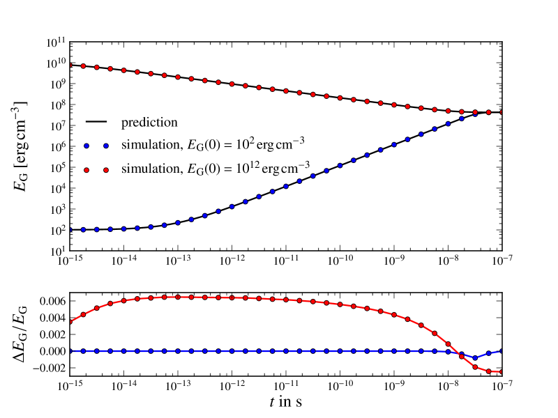
Figure 3: Results of the equilibration simulations described in Section 4.2. The blue symbols show the results of the Monte Carlo simulation with an initial internal energy density of $E_{\mathrm{G}}(0)=10^{2}\,\mathrm{erg\,cm^{-3}}$ for a series of selected snapshots. The corresponding results obtained for the initial energy density of $E_{\mathrm{G}}(0)=10^{10}\,\mathrm{erg\,cm^{-3}}$ are shown with red circles. The temporal evolution of the internal energy density as predicted by Equation (49) for both cases is indicated by the solid black lines. The initial radiation field energy density is set to $E_{\mathrm{R}}(0)=10^{12}\,\mathrm{erg\,cm^{-3}}$ in both simulations. In the lower panel, the relative difference between the theoretically expected ($E_{\mathrm{th}}$) and the simulated ($E_{\mathrm{sim}}$) evolution of the internal energy density, $(E_{\mathrm{th}}-E_{\mathrm{sim}})/E_{\mathrm{th}}$, is shown for both calculations.

In a second test calculation, the initial radiation field energy content was set to zero and the internal energy density to $E_{\mathrm{G}}(0)=10^{8}\,\mathrm{erg\,cm}^{-3}$. The remaining simulation parameters are adopted from the previous equilibration setup. Over time, the fluid will drive the radiation field towards equilibrium by the emission of thermal photons. To theoretically predict the evolution of the radiation-matter state, the coupled differential Equations (50) and (49) can be solved simultaneously by numerical integration. In contrast to the previous simulations, neither the radiation temperature, nor the gas temperature can be assumed to be constant. In Fig. 4, the results of our Monte Carlo simulation are tested against the theoretically predicted evolution. Again, only systematic deviations, which are caused by the finite duration of the simulation time steps, persist on the per cent level.

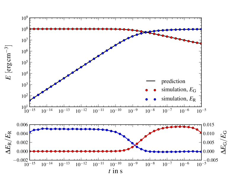
Figure 4: Equilibration calculation with an initially absent radiation field and a starting internal energy density of $E_{\mathrm{G}}=10^{8}\,\mathrm{erg\,cm^{-3}}$. For a series of selected time snapshots, the theoretical evolution of this system, obtained by numerically integrating Equations (50) and (49) is displayed as black lines. The corresponding results form our Monte Carlo simulation are depicted as blue and red circles for the radiative and internal energy density, respectively. As in Fig. 3, the relative difference between the theoretically expected and the simulated energy evolution is shown in the lower panel.

The agreement between our test calculations and the theoretically predicted behaviour for the relaxation towards equilibrium is excellent as illustrated in Figs. 3 and 4, indicating that our numerical methods describing the matter-radiation interactions and their implementation are accurate and work correctly.

4.3 Radiative Shocks

The calculations presented above probed the propagation of the radiation field, the basic interaction machinery and the determination of heating and cooling terms, neglecting any effects of radiation and thermodynamic pressure and the fluid motion. In our final, most challenging test, we verify that the interaction processes and our approach as a whole yield the correct radiation-hydrodynamical coupling. For this purpose we examine sub- and supercritical radiative shocks. The seminal works describing this type of shocks analytically date back to Zel’dovich (1957a) and Raizer (1957a) and to Marshak (1958). The results of the two former studies are summarized in detail by Zel’dovich & Raizer (1967).

Radiative shocks exhibit a structure and dynamical behaviour that is very different from their purely hydrodynamical counterparts, due to the presence of a radiative precursor. The pre-shock material is heated by the flow of radiative energy through the shock front. Depending on the strength of the shock and in turn on the amount of heating of the pre-shock material, two classes of radiative shocks can be distinguished. Following the discussion of Mihalas & Mihalas (1984), we denote the gas temperature behind the shock front with $T_{2}$ and immediately in front of it with $T_{-}$. In the case of $T_{-}$ being much lower than $T_{2}$, due to the small amount of pre-heating, a sub-critical shock is encountered. With increasing shock strength, equivalent to the shock front moving faster, the radiative precursor heats the material more and more until it reaches the critical configuration of $T_{-}=T_{2}$. At this point, a further increase in the shock strength only results in a deeper penetration of the radiation precursor. Consequently, $T_{-}$ never surpasses the temperature behind the front in such supercritical shocks.

The structure of radiative shocks has already been determined in various numerical studies, including works by Heaslet & Baldwin (1963) and Sincell et al. (1999). Following the proposal of Ensman (1994), these shocks have been used as a common test problem to verify the accuracy of numerical approaches to radiation hydrodynamics. In particular, the realisation of the matter-radiation coupling in the zeus-code has been tested extensively using radiative shocks (Turner & Stone, 2001; Hayes & Norman, 2003; Hayes et al., 2006). For comparison to our Monte Carlo radiation-hydrodynamical simulations, we will use results calculated with the latest version of this code, zeus-mp2 (Hayes et al., 2006).

For the calculation of sub- and supercritical radiative shocks we choose the properties of the radiating fluid according to Hayes et al. (2006) which in turn were motivated by the simulations performed by Ensman (1994). In particular, a one-dimensional plane-parallel domain of length $7\times 10^{10}\,\mathrm{cm}$ and a fluid with initial density of $7.78\times 10^{-8}\,\mathrm{g\,cm}^{-3}$ is considered. The temperature is set to $85\,\mathrm{K}$ at the inner, reflecting boundary and decreased linearly to $10\,\mathrm{K}$ at the outer open boundary of the domain. We adopt this profile to facilitate comparison with the calculations performed by Ensman (1994), in which a temperature gradient had to be imposed for reasons of numerical stability. Throughout the domain, a uniform grey absorption opacity of $3.1\times 10^{-10}\,\mathrm{cm}^{-1}$ is chosen, resulting in a photon mean free path that is roughly 20 times shorter than the extent of the computational box. The shock is created by driving the material into the reflecting inner boundary with a bulk velocity of $-6\,\mathrm{km\,s}^{-1}$ for the sub-critical case and with $-20\,\mathrm{km\,s}^{-1}$ for the supercritical calculation, respectively. We determine the evolution of the resulting radiative shocks with our Monte Carlo program and as a reference with the zeus-mp2 code. Figs. 5 and 6 show comparisons between the gas and radiation temperature structures calculated with both codes for the sub- and the supercritical shocks respectively. To be compatible with Ensman (1994) we display the shock structure in the rest frame coordinates of the un-shocked material (Hayes & Norman, 2003; Hayes et al., 2006).

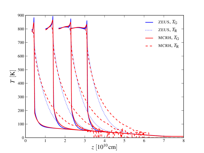
Figure 5: Temperature profiles of a sub-critical radiative shock calculated with our Monte Carlo radiation hydrodynamics (red lines) program and the zeus-mp2 code (blue lines). The gas temperature is depicted with solid lines, while the radiation temperature is shown as dashed and dotted lines. Profiles are shown for $t=5.4\times 10^{3}$, $1.7\times 10^{4}$, $2.8\times 10^{4}$ and $3.8\times 10^{4}\,\mathrm{s}$ and are plotted in the rest frame of the un-shocked material. Note the Monte Carlo noise in the radiation temperature ahead of the shock. Here, the radiation field is only represented by a small number of packets.

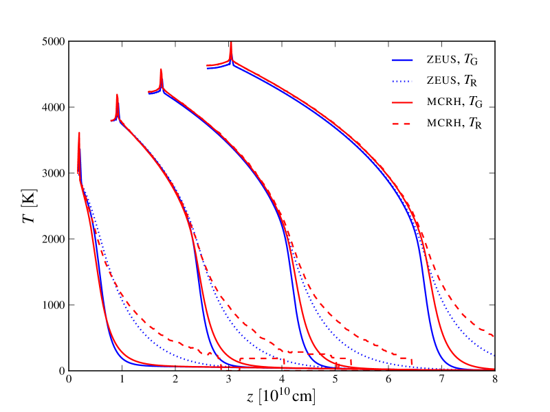
Figure 6: Analogous to Fig. 5 but now displaying the corresponding calculation of the supercritical shock. The results from the Monte Carlo simulation are again shown in red and the ones obtained with zeus-mp2 in blue. Gas and radiation temperature are indicated with solid and dashed/dotted lines respectively and shown with respect to the un-shocked material. Temperature profiles are presented for $t=8.6\times 10^{2}$, $4.0\times 10^{3}$, $7.5\times 10^{3}$ and $1.3\times 10^{4}\,\mathrm{s}$.

As shown in Figs. 5 and 6, the radiative shocks calculated with our mcrh code exhibit the expected overall structure and characteristic features. In the subcritical case, a weak radiative precursor leads to mild heating of the pre-shock material. The effect of the precursor is much more prominent in the second case of the supercritical shock. Here, the sharp shock front is washed out by the strong heating of the upstream material by the radiative flux penetrating the pre-shock domain. As predicted for supercritical shocks, the material immediately ahead of the shock is heated significantly, reaching the same temperature as behind the front. Overall, our numerical results agree very well with the zeus-mp2 calculations, especially with respect to the location of the shock and the gas temperature profiles. However, our Monte Carlo simulations predict a stronger and deeper penetration of the unshocked material by the radiation field. This results in increased heating of the material and differences in the radiation temperature profiles with respect to the zeus-mp2 results. These differences are most likely caused by the simplifications implemented in the zeus-mp2 code, which treats the radiative flux in the diffusion approximation, augmented by the introduction of a flux limiter (see Hayes et al., 2006, equation 11). The influence of this simplified scheme on the structure of radiative shocks has already been studied by Ensman (1994). Calculating the evolution of a supercritical shock on the one hand by relying on the diffusion approximation and on the other hand by solving the radiation-hydrodynamical equations without any simplifications directly, revealed the same behaviour of the radiative precursor (see Ensman, 1994, fig. 15). Despite its statistical nature, the Monte Carlo approach provides a direct solution to the transfer equation without introducing any physical simplifications. For these reasons we believe that the differences are due to the employed methods and not a shortcoming of our approach to radiation hydrodynamics.

The test calculations presented in this section have been carried out without using the smoothing capability of our program (see Section 3.11). In the simulations determining the structure of radiative shocks, the noise suppression of the volume-based estimator approach was sufficient to accurately resolve the heating effects in the precursor regime with large deviations from LTE. For example, in our simulation of the subcritical shock a maximum of $6\times 10^{5}$ packets were active at a time, simulating the evolution of the radiation field. However, as anticipated in Sections 3.3 and 3.11, in the regions around the shock front, where the radiation field is close to LTE, the radiation force components are subject to non-negligible statistical fluctuations. But this noise component is effectively suppressed on the characteristic hydrodynamical time scales, due to a high packet recycling rate. Typically, the entire packet ensemble is re-populated multiple times during a radiative transfer step, causing a smooth temperature profile even in the near-LTE regions.

With the calculations presented in this section, the different individual mechanisms of our method have been successfully tested and the correct radiation-hydrodynamical behaviour of the approach as a whole has been demonstrated without applying any smoothing. A first application to an astrophysical environment is presented in the next Section.

5 Application

Our framework has been specifically designed to address radiation-hydrodynamical problems in astrophysical systems with large outflows such as supernova (SN) explosions. To verify our approach for problems of astrophysical interest, we consider the homologous expansion phase of SN Ia ejecta.

In the expelled material of SNe Ia, radioactive decays emit $\gamma$-rays, which interact strongly with the ejecta. This coupling affects the expansion dynamics leading to changes in the density and velocity profile that could influence the observable display. The question of whether this radiation-hydrodynamical effect is important for theoretical determinations of SN light curves and spectra has already been addressed by Pinto & Eastman (2000) using a series of analytical estimates. This study concluded, that the radiative influence on the expansion of the ejecta is marginal and does not cause significant changes in the light curve. These findings were verified in the study of Woosley et al. (2007), which involved detailed radiation-hydrodynamical calculations with the stella code (Blinnikov et al., 2006). Changes on a 10 per cent level in the density stratification of the ejecta were identified when including the radiation-matter coupling. Here, we re-address this problem for the purpose of testing our radiation-hydrodynamical approach in astrophysical environments.

5.1 Code Extensions

For the application to supernova ejecta, our program is extended to account for the energy release accompanying radioactive decays. The determination of the energy injection into the radiation field involves tracking the abundances of $\mathrm{{}^{56}Ni}$ and its daughter nucleus $\mathrm{{}^{56}Co}$. Both radio-nuclides are proton-rich and decay through electron-capture reactions down to stable $\mathrm{{}^{56}Fe}$. These decay reactions occur on the characteristic $e$-folding time scales of $t_{\mathrm{Ni}}=8.80\,\mathrm{d}$ for $\mathrm{{}^{56}Ni}\rightarrow\mathrm{{}^{56}Co}$ and $t_{\mathrm{Co}}=113.7\,\mathrm{d}$ for $\mathrm{{}^{56}Co}\rightarrow\mathrm{{}^{56}Fe}$ and are accompanied by a cascade of $\gamma$-ray emissions. The $\gamma$-photons interact with the surrounding material through Compton-scattering, production of $e^{+}e^{-}$ pairs and the photoelectric effect. As a result of these interaction mechanisms, the $\gamma$-radiation heats the surrounding material and the energy is re-radiated as quasi-thermal emission. Assuming instant thermalisation we simplify the $\gamma$-interaction processes by relying only on one effective absorptive opacity (Sutherland & Wheeler, 1984; Swartz et al., 1995). We model the net effect of injecting energy into the thermal radiation field by a grey Monte Carlo transport step. For each simulation time step, the number of radioactive decays is determined and an adequate number of Monte Carlo packets representing the emitted $\gamma$-energy is created. For this purpose we follow Lucy (2005) and integrate over the $\gamma$-spectrum of the decay reactions (see Ambwani & Sutherland, 1988, table 1), obtaining a total energy release in the form of $\gamma$-radiation of $E_{\mathrm{Ni}}=1.728\,\mathrm{MeV}$ and $E_{\mathrm{Co}}=3.566\,\mathrm{MeV}$ per decaying $\mathrm{{}^{56}Ni}$ and $\mathrm{{}^{56}Co}$ nucleus respectively. The $\gamma$-packets propagate in the same manner as the Monte Carlo packets describing the thermal radiation field, but the interactions with the ejecta material are described by different opacities. Each $\gamma$-packet that undergoes an absorption is automatically transformed into a thermal radiation packet, which is then treated according to the methods laid out in Section 3.8.

5.2 Toy Simulations

To verify the correct operation and the validity of the adopted simplified treatment of the radioactive energy injection, we present the results of a simple toy simulation following Lucy (2005). In his study, Lucy developed a Monte Carlo radiative transfer method to determine spectra and light curves in SNe Ia. In the verification process, Lucy performed a grey radiative transfer simulation for a simplified ejecta structure under the assumption of homologous expansion. A comparison of the bolometric light curve determined in the Monte Carlo simulation with the results of a moments-equation solution technique (Castor, 1972) yielded excellent agreement. Using the results of Lucy (2005) as a reference, we test the implementation of the radioactive decay mechanism and the $\gamma$-transport module in our Monte Carlo radiation hydrodynamics program. In addition, this simulation provides yet another test for the accurate operation of the Monte Carlo radiative transfer procedures. Particularly, the determination of the emergent light curve is sensitive to the correct implementation of first-order relativistic effects, such as angle aberration and Doppler-shifts, due to the high ejecta velocities in this application. The parameters for this test calculations, as described in Lucy (2005), are adopted from a model SN presented in Pinto & Eastman (2000). We consider a SN with a total ejecta mass of $M=1.39M_{\odot}$. The ejecta are in homologous expansion with a maximum velocity of $u_{\mathrm{max}}=10^{4}\,\mathrm{km\,s}^{-1}$ and a uniform density of $\rho=3.79\times 10^{-11}\,\mathrm{g\,cm}^{-3}$. In the ejecta, the radioactive $\mathrm{{}^{56}Ni}$ is assumed to be strongly concentrated in the core, resulting in a $\mathrm{{}^{56}Ni}$ distribution of $f_{\mathrm{Ni}}(M_{r})=1$ for $M_{r}<0.5\,M_{\odot}$ that linearly drops to zero at $M_{r}=0.75\,M_{\odot}$. Here, $M_{r}$ denotes the mass contained within a sphere of radius $r$. Throughout the entire material, a constant interaction opacity for the thermal radiation field of $\chi/\rho=0.1\,\mathrm{cm^{2}\,g^{-1}}$ is used. Following Lucy (2005), we assume radiative equilibrium which allows us to simplify the interaction mechanism to only include scattering events. The grey absorption cross section for $\gamma$-radiation of $\kappa_{\gamma}/\rho=0.03\,\mathrm{cm^{2}\,g^{-1}}$ is adopted from Sutherland & Wheeler (1984) and Ambwani & Sutherland (1988).

We start the Monte Carlo simulation at $t=3.0\,\mathrm{d}$. At much earlier times, the high optical thickness of the ejecta material prevents an efficient use of the Monte Carlo radiative transfer methods. We bridge the time between the explosion to the start of the simulation by an analytic homologous expansion calculation. Here, we assume that the entire energy released in the radioactive decay reactions of $\mathrm{{}^{56}Ni}$ and $\mathrm{{}^{56}Co}$ immediately thermalises, raising the gas temperature to the values shown in Fig. 7 at the time of the onset of the Monte Carlo simulation.

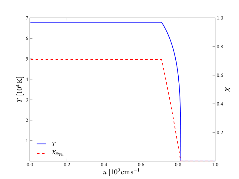
Figure 7: Initial conditions for our Monte Carlo simulation of the Lucy (2005) model SN ejecta at $t=3.0\,\mathrm{d}$. The time before the onset of the simulation was bridged by an analytic homologous expansion calculation, resulting in the temperature profile shown as a blue solid line. The dashed red line describes the distribution of $\mathrm{{}^{56}Ni}$.

This figure also illustrates the distribution of radioactive $\mathrm{{}^{56}Ni}$ after the initial homologous expansion phase. Since the calculations of Lucy (2005) did not include any radiation-hydrodynamical coupling, this interaction mechanism was also switched off in our test simulation. Consequently, the radiative transfer is not affecting the homologous expansion of the ejecta material.

Fig. 8 presents the bolometric light curve determined in our Monte Carlo simulation and shows the comparison with the results of Lucy (2005).

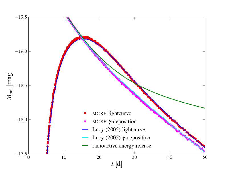
Figure 8: Comparison between the bolometric light curve calculated with our Monte Carlo program (red) and the results of the Lucy (2005) calculation (blue). In addition, the rate at which the $\gamma$ radiation deposits its energy in the thermal radiation field is illustrated for both calculations (magenta and cyan). As a reference, the actual energy release in the decay reactions in the form of $\gamma$ radiation is also shown as the green line.

The excellent agreement between our simulation and the calculations performed by Lucy (2005) demonstrates the operation of the energy injection process together with the $\gamma$-transport scheme and once more verifies the accurate performance of our Monte Carlo approach as a whole.

5.3 Application to the W7-Model

With the SN specific extensions, our program is well suited to examine the influence of the radiation-hydrodynamical coupling on the observed bolometric light curve. For this purpose we consider a SN that is described by the well-known W7 model, first presented by Nomoto et al. (1984) and extended by larger nuclear networks in the studies of Thielemann et al. (1986) and Iwamoto et al. (1999). This parameterized one-dimensional SN Ia explosion model reproduces important observables and has thus become a standard reference in the literature. Nomoto et al. (1984) determined the evolution of the fluid dynamical state of the ejecta material until $t=20\,\mathrm{s}$ after the ignition of the thermonuclear explosion. Characteristic for the W7 model is the concentration of the bulk of the $\mathrm{{}^{56}Ni}$ in an extended shell, spanning the velocity region from $3\times 10^{8}\,\mathrm{cm\,s^{-1}}$ to $10^{9}\,\mathrm{cm\,s^{-1}}$, instead of being concentrated in the core. To accurately resolve this $\mathrm{{}^{56}Ni}$ shell, we discretize the original W7 profile to a one-dimensional spherical grid with 2000 equidistant cells. In addition, we slightly adjust the velocity profile of the original model to match exactly the homology condition, allowing us to make a clear and unperturbed identification of the influence of the radiation-matter coupling on the ejecta dynamics. As in our calculation for the Lucy (2005) toy model, we start the Monte Carlo radiation hydrodynamics calculation at $t=3\,\mathrm{d}$ assuming perfect homologous expansion behaviour of the ejecta up to this point. The resulting temperature profile after this pure homologous phase at $t=3\,\mathrm{d}$ is shown in Fig. 9 together with the distribution of $\mathrm{{}^{56}Ni}$. The density stratification at this time is visualised in Fig. 10.

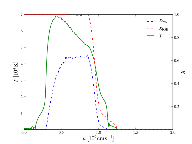
Figure 9: The temperature profile (green line) of the W7 model after discretization of the original data set onto a spherical grid of 2000 cells and performing an homologous expansion calculation up to $t=3\,\mathrm{d}$ after explosion. In addition, the mass fraction of the radioactive $\mathrm{{}^{56}Ni}$ is illustrated with the dashed blue line. It illustrates the characteristic concentration of the $\mathrm{{}^{56}Ni}$ in the extended shell in the intermediate ejecta regions of the W7 model ($3\times 10^{8}\,\mathrm{cm\,s^{-1}}<u<10^{9}\,\mathrm{cm\,s^{-1}}$). All elements with $Z\geq 20$ are denoted as iron group elements (IGE) whose combined distribution is shown as the red dashed line.

In analogy to the model simulation presented in Section 5.2 we follow Lucy (2005) and assume that the ejecta material is in radiative equilibrium. Consequently, we can simplify the interaction mechanism between the thermal radiation field and the surrounding material by a pure scattering description. The grey scattering opacity is not constant throughout the ejecta radius, but follows the distribution of heavy elements, which constitute the dominant opacity source for the thermal radiation photons. In particular, we follow Mazzali & Podsiadlowski (2006) and Sim (2007) in setting the scattering opacity to

$$\chi/\rho=N(0.9X_{\mathrm{IGE}}+0.1),$$ (51)

where the iron group (IGE) involves all elements heavier than calcium (the combined distribution of these elements can be read off from Fig. 9). The scaling factor $N$ is chosen to ensure a mean interaction cross section of $\langle\chi/\rho\rangle=0.1\,\mathrm{cm^{2}\,g^{-1}}$. Fig. 10 shows the effect of the heavy elements on the interaction cross section throughout the ejecta material.

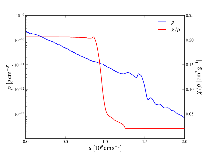
Figure 10: The density profile of the W7 model at the start of our Monte Carlo simulation at $t=3\,\mathrm{d}$ (blue, left scale) and the scattering cross-section per gram (red, right scale) obtained from Equation (51).

All interactions of the $\gamma$-radiation are described by a single constant absorption opacity of $\kappa_{\gamma}/\rho=0.03\,\mathrm{cm^{2}\,g^{-1}}$ (see Section 5.2). With these parameters, the temporal evolution of the hydrodynamical state of the W7 ejecta is calculated up to $t=45\,\mathrm{d}$. Fig. 11 illustrates the behaviour of the radiation field, quantified by the mean intensity $J$, during this period of time.

Figure 11: Temporal evolution of the mean intensity of the radiation field in the radiation-hydrodynamical simulation of the W7 model. Initially, the radiation field is confined to the $\mathrm{{}^{56}Ni}$ shell but with decreasing optical depth it penetrates the inner and outer regions of the ejecta.

At the beginning, the radiation field is concentrated at the location of the $\mathrm{{}^{56}Ni}$-shell, where initially most of the $\gamma$-interactions take place due to the high optical depth of the ejecta. As time progresses, the ejecta become increasingly transparent to the radiation field, which begins to penetrate the inner regions and propagates to the outer edge of the supernova ejecta. Here, the Monte Carlo packets escape and are recorded to determine the bolometric light curve. Due to the radiation pressure, the initially confined radiation field leaves imprints on the velocity and density profiles of the ejecta material as it propagates in- and outwards. The changes in the ejecta structure are indicated in Fig. 12,

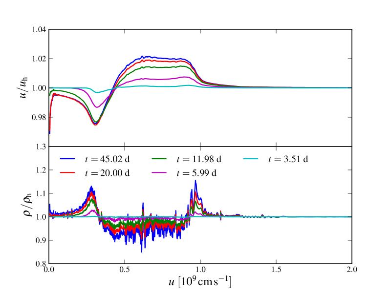
Figure 12: Illustration of the influence of the radiation field on the evolution of the fluid state. In the upper panel, the velocity profile in the ejecta is displayed with respect to a purely homologous expansion for a variety of temporal snapshots (see labels in figure). In the lower panel, the density stratification is displayed in a corresponding fashion. The de- and accelerating effects of the radiation pressure are clearly visible in the velocity profiles, as is the resulting dilution of the $\mathrm{{}^{56}Ni}$ shell in the lower panel.

which shows the velocity and density profiles with respect to a purely homologous expansion that would occur in the absence of the radiation-hydrodynamical coupling. The radiation pressure accelerates the ejecta motion in the outer parts of the $\mathrm{{}^{56}Ni}$ shell and decelerates the expansion in the inner regions. Both effects dilute the $\mathrm{{}^{56}Ni}$ shell and pile up material at the edges of this region. The influence of the radiation pressure is strongest in the early phases of the expansion, where the high optical depth causes a strong coupling of the radiation field to the surrounding material and stalls as the ejecta become more and more transparent. In total, the radiation pressure induces deviations from the purely homologous density profile on the order of 10 per cent, which are compatible with the findings of the previous study by Woosley et al. (2007). The structural changes in the density stratification are, however, not prominent enough to significantly alter the shape of the emergent bolometric light curve. Neglecting the radiation-hydrodynamical coupling and assuming a purely homologous expansion yields nearly the same bolometric light curve as a detailed calculation. A comparison of both simulations is shown in Fig. 13.

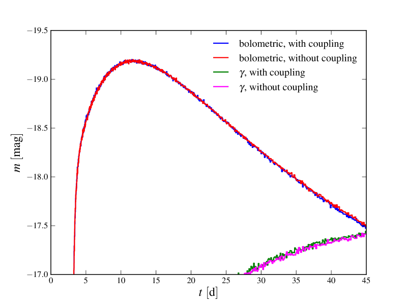
Figure 13: Comparison between bolometric light curves calculated for the W7 model with the radiation-hydrodynamical coupling (blue line) and with a pure radiative transfer calculation and homologous expansion of the ejecta material (red line). The emergent $\gamma$-light curve is also displayed for both simulations (green and cyan, respectively). No significant influence of the radiation-matter coupling or the resulting changes in the ejecta structure can be identified in the bolometric light curves.

Even if the bolometric light curve remains unaffected by changes in the fluid state, colour light curves may be affected since the radiation pressure changes the velocity of ejecta regions in which different elements are concentrated. However, this effect cannot be studied with the current grey implementation of our approach to radiation hydrodynamics and remains to be re-addressed with a chromatic version of the code.

All simulations presented in this section required about $3.5\times 10^{13}$ floating point operations. In these calculations the initial radiation field at $t=3\,\mathrm{d}$ was discretized by $10^{6}$ Monte Carlo packets. Due to the energy release in the decay reactions and the outflow of radiation packets at the outer edge of the ejecta, the number of active packets varied greatly during the simulation, but a maximum of $2.43\times 10^{6}$ packets were used to represent the radiation field at any time.

Despite the large number of packets, the Monte Carlo estimators for the radiation force are subject to a significant level of statistical noise. In this particular case, the entire energy-momentum transfer is determined by the radiative flux in the co-moving frame (cf. Equations 42 and 43). As pointed out in Sections 3.3 and 3.11, our discretization approach is not ideally suited to accurately capture this quantity in regions where the radiation field is nearly isotropic, such as the inner parts of the $\mathrm{{}^{56}Ni}$ shell. However, despite being subject to a considerable level of Monte Carlo noise, the radiative flux captures the expected effect of the radiation field inflating the $\mathrm{{}^{56}Ni}$ bubble (see Figure 14). Thus, we employed a smoothing kernel (cf. Section 3.11) in our simulations, averaging over 30 neighbouring cells and thereby avoiding difficulties in the hydrodynamical solver. In the absence of this smoothing, cell-to-cell fluctuations in the fluid state lead to convergence problems in the Riemann solver that could not be averted by increasing the number of active packets on computationally feasible scales. Using the smoothing capability gives a significant reduction of the cell-to-cell fluctuations without damaging the physical variations in the quantities, as Fig. 14 illustrates. Here, the density stratification at $t=14.3\,\mathrm{d}$ is shown for both a simulation that includes smoothing over 30 neighbouring cells and for one with very mild smoothing over 3 cells only, proving that the approach preserves the physical signal.

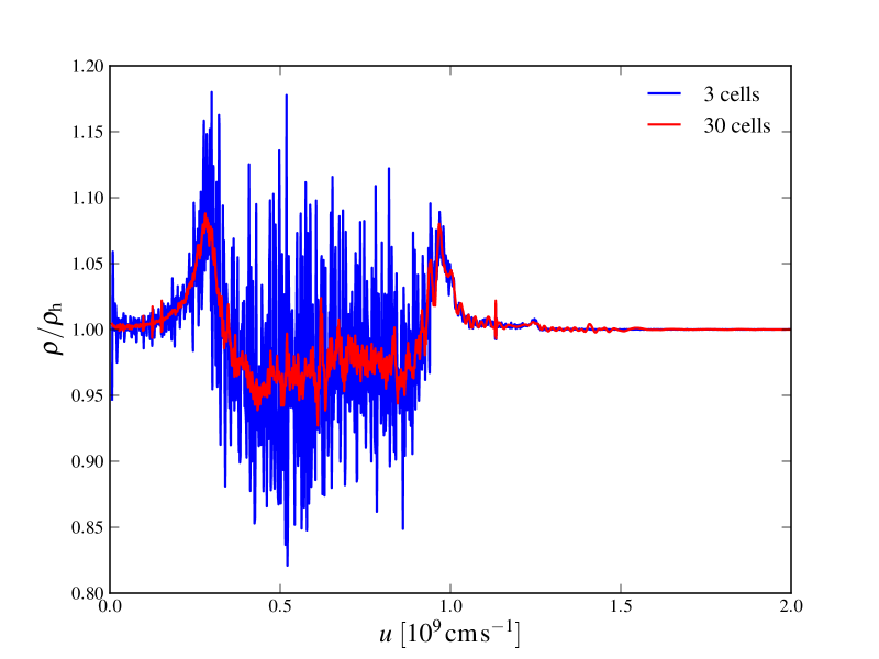
Figure 14: Illustration of the influence of smoothing on the density evolution of the ejecta. The density profiles at $t=14.3\,\mathrm{d}$ are displayed with respect to a purely homologous expansion (cf. Fig .12). We show the results of two simulations: one that employs smoothing over the neighbouring 30 cells (red line) and one with very mild smoothing over 3 cells (blue line). As this comparison shows, the smoothing approach removes the strong stochastic cell-to-cell fluctuations, but retains the overall physical variation.

6 Discussion

In this paper we presented a Monte Carlo approach to radiation hydrodynamical problems in astrophysical environments. By combining Monte Carlo radiative transfer methods that rely on the indivisible packet formalism (Abbott & Lucy, 1985) with the finite-volume hydrodynamical technique PPM (Colella & Woodward, 1984) we have aimed to retain the benefits of the Monte Carlo machinery for the modelling of complex interaction physics and arbitrary geometries. Here, our main focus lay on the development and presentation of the necessary numerical tools and on demonstrating the operation of this method, its physical accuracy and its computational feasibility. By using volume-based Monte Carlo estimators (Lucy, 1999, 2002, 2003) in the reconstruction of radiation field characteristics, the maximum amount of information is extracted from the propagation behaviour of Monte Carlo packets and the Monte Carlo noise is minimized.

A series of toy calculations has been performed to test the operation of the main components of our Monte Carlo radiation hydrodynamical method. In particular, the simulation of radiative shocks verified the accuracy of our approach to a standard radiation hydrodynamical test. As expected, due to the nature of the Monte Carlo method, calculations in optically thick environments are time-consuming but feasible and accurate, as the radiative shock examples showed. In general, all calculations were completed within hours to a day on a single desktop CPU. However, due to the very efficient scaling behaviour of the Monte Carlo algorithm to large numbers of processor cores, a future parallel implementation of the method provides the scope for significant decreases in the run time.

The application to SN Ia ejecta successfully demonstrated the operation of our method to an astrophysical problem for which this method was primarily developed. In this exercise, the influence of the radiation-matter coupling on the density stratification during the near-homologous expansion phase of the ejecta has been investigated. The results we obtained are in agreement with the previous study by Woosley et al. (2007) who used the radiation hydrodynamics code stella (Blinnikov et al., 2006). The induced changes in the ejecta structure, however, were confirmed to have no significant influence on the bolometric light curve, as predicted by Pinto & Eastman (2000).

Despite the agreement of our results with previous studies, the SN Ia application also illustrated some difficulties of our approach. Our discretization scheme into packets of radiative energy allows us to easily construct all relevant radiation field characteristics and can be generalized to a fully frequency-dependent transport treatment in a straight-forward manner. However, in regions where the radiation field is close to LTE or to isotropy, the radiation force components are subject to considerable statistical fluctuations due to this discretization choice. Here, we suppressed this noise component by applying a smoothing kernel. Although beyond the scope of this work, in the future further reduction of the statistical noise should be explored by incorporating implicit Monte Carlo techniques (Fleck & Cummings, 1971) or a Monte Carlo radiative transfer approach that is based on the difference formulation (Szöke & Brooks, 2005; Brooks et al., 2005). For such schemes, it will be important to consider how all the physical processes necessary to adequately address particular astrophysical applications can be implemented.

As the main aim of this work was to establish the methods and the numerical framework of the Monte Carlo radiation hydrodynamics approach, all calculations were performed with a simplified implementation of the method. In particular, we restricted our tests to one-dimensional geometries and the radiative transfer was performed in a grey approximation with a very simple opacity prescription. However, we stress that these simplifications were made only to reduce the complexity and the computational effort of the test simulations. They do not affect the applicability and operation of the Monte Carlo radiation hydrodynamical approach itself. In the future, we aim to introduce more sophisticated opacity prescriptions and make the transition from grey transport to a fully frequency-dependent radiative transfer scheme. This will add a further level of sophistication to the method, but will not impact the operation of the radiation-matter coupling in our approach. The tools to realise the frequency-dependent transfer have already been developed and are provided for example in the framework of the macro-atom formalism by Lucy (2002). In addition to improving the physical accuracy of the radiative transfer, our long-term efforts will be directed towards a generalised implementation for multi-dimensional problems. With this generalization our radiation hydrodynamical method will include all major capabilities that have already made the Monte Carlo technique a very successful and rewarding approach for pure radiation transport applications.

References

- Abbott & Lucy (1985) Abbott D. C., Lucy L. B., 1985, ApJ, 288, 679
- Ambwani & Sutherland (1988) Ambwani K., Sutherland P., 1988, ApJ, 325, 820
- Asplund et al. (2000) Asplund M., Nordlund Å., Trampedach R., Allende Prieto C., Stein R. F., 2000, A&A, 359, 729
- Avery & House (1968) Avery L. W., House L. L., 1968, ApJ, 152, 493
- Blinnikov et al. (2000) Blinnikov S., Lundqvist P., Bartunov O., Nomoto K., Iwamoto K., 2000, ApJ, 532, 1132
- Blinnikov et al. (2006) Blinnikov S. I., Röpke F. K., Sorokina E. I., Gieseler M., Reinecke M., Travaglio C., Hillebrandt W., Stritzinger M., 2006, A&A, 453, 229
- Brooks et al. (2005) Brooks E. D., McKingley M. S., Daffin F., Szöke A., 2005, Journal of Computational Physics, 205, 737
- Carciofi & Bjorkman (2006) Carciofi A. C., Bjorkman J. E., 2006, ApJ, 639, 1081
- Castor (1972) Castor J. I., 1972, ApJ, 178, 779
- Colella & Woodward (1984) Colella P., Woodward P. R., 1984, Journal of Computational Physics, 54, 174
- Edelmann (2010) Edelmann P. V. F., 2010, Master’s thesis, Technische Universität München
- Ensman (1994) Ensman L., 1994, ApJ, 424, 275
- Ercolano et al. (2003) Ercolano B., Barlow M. J., Storey P. J., Liu X.-W., 2003, MNRAS, 340, 1136
- Fleck & Cummings (1971) Fleck J. A., Cummings J. D., 1971, Journal of Computational Physics, 8, 313
- Fryer et al. (2010) Fryer C. L., Ruiter A. J., Belczynski K., Brown P. J., Bufano F., Diehl S., Fontes C. J., Frey L. H., Holland S. T., Hungerford A. L., Immler S., Mazzali P., Meakin C., Milne P. A., Raskin C., Timmes F. X., 2010, ApJ, 725, 296
- Garcia-Segura et al. (1996) Garcia-Segura G., Mac Low M.-M., Langer N., 1996, A&A, 305, 229
- Godunov (1959) Godunov S. K., 1959, Matematicheskii Sbornik, 47, 271
- Harries (2011) Harries T. J., 2011, MNRAS, 416, 1500
- Hayes & Norman (2003) Hayes J. C., Norman M. L., 2003, ApJS, 147, 197
- Hayes et al. (2006) Hayes J. C., Norman M. L., Fiedler R. A., Bordner J. O., Li P. S., Clark S. E., ud-Doula A., Mac Low M.-M., 2006, ApJS, 165, 188
- Heaslet & Baldwin (1963) Heaslet M. A., Baldwin B. S., 1963, Physics of Fluids, 6, 781
- Hirose et al. (2009) Hirose S., Krolik J. H., Blaes O., 2009, ApJ, 691, 16
- Höflich & Schaefer (2009) Höflich P., Schaefer B. E., 2009, ApJ, 705, 483
- Iwamoto et al. (1999) Iwamoto K., Brachwitz F., Nomoto K., Kishimoto N., Umeda H., Hix W. R., Thielemann F., 1999, ApJS, 125, 439
- Jack et al. (2011) Jack D., Hauschildt P. H., Baron E., 2011, A&A, 528, A141
- Janka & Mueller (1996) Janka H., Mueller E., 1996, A&A, 306, 167
- Kasen (2010) Kasen D., 2010, ApJ, 708, 1025
- Kasen et al. (2006) Kasen D., Thomas R. C., Nugent P., 2006, ApJ, 651, 366
- Kasen et al. (2011) Kasen D., Woosley S. E., Heger A., 2011, ApJ, 734, 102
- Kromer & Sim (2009) Kromer M., Sim S. A., 2009, MNRAS, 398, 1809
- Kuiper et al. (2010) Kuiper R., Klahr H., Dullemond C., Kley W., Henning T., 2010, A&A, 511, A81
- LeVeque (2002) LeVeque R. J., 2002, Finite-Volume Methods for Hyperbolic Problems. Cambridge University Press
- Levermore & Pomraning (1981) Levermore C. D., Pomraning G. C., 1981, ApJ, 248, 321
- Long & Knigge (2002) Long K. S., Knigge C., 2002, ApJ, 579, 725
- Lucy (1999) Lucy L. B., 1999, A&A, 344, 282
- Lucy (2002) Lucy L. B., 2002, A&A, 384, 725
- Lucy (2003) Lucy L. B., 2003, A&A, 403, 261
- Lucy (2005) Lucy L. B., 2005, A&A, 429, 19
- Lucy & Abbott (1993) Lucy L. B., Abbott D. C., 1993, ApJ, 405, 738
- Marshak (1958) Marshak R. E., 1958, Physics of Fluids, 1, 24
- Marti et al. (1997) Marti J. M. A., Mueller E., Font J. A., Ibanez J. M. A., Marquina A., 1997, ApJ, 479, 151
- Mazzali & Lucy (1993) Mazzali P. A., Lucy L. B., 1993, A&A, 279, 447
- Mazzali & Podsiadlowski (2006) Mazzali P. A., Podsiadlowski P., 2006, MNRAS, 369, L19
- Mellema & Lundqvist (2002) Mellema G., Lundqvist P., 2002, A&A, 394, 901
- Mihalas & Mihalas (1984) Mihalas D., Mihalas B. W., 1984, Foundations of radiation hydrodynamics
- Noebauer et al. (2010) Noebauer U. M., Long K. S., Sim S. A., Knigge C., 2010, ApJ, 719, 1932
- Nomoto et al. (1984) Nomoto K., Thielemann F., Yokoi K., 1984, ApJ, 286, 644
- Pincus & Evans (2009) Pincus R., Evans K. F., 2009, Journal of Atmospheric Sciences, 66, 3131
- Pinto & Eastman (2000) Pinto P. A., Eastman R. G., 2000, ApJ, 530, 744
- Piro et al. (2010) Piro A. L., Chang P., Weinberg N. N., 2010, ApJ, 708, 598
- Raizer (1957a) Raizer Y. P., 1957a, Zh. Eksp. Teor. Fiz., 32, 1528
- Raizer (1957b) Raizer Y. P., 1957b, Soviet Physics JETP, 5, 1242
- Röpke & Hillebrandt (2005) Röpke F. K., Hillebrandt W., 2005, A&A, 431, 635
- Sim (2005) Sim S. A., 2005, MNRAS, 356, 531
- Sim (2007) Sim S. A., 2007, MNRAS, 375, 154
- Sincell et al. (1999) Sincell M. W., Gehmeyr M., Mihalas D., 1999, Shock Waves, 9, 391
- Stein & Nordlund (1998) Stein R. F., Nordlund A., 1998, ApJ, 499, 914
- Sundqvist et al. (2010) Sundqvist J. O., Puls J., Feldmeier A., 2010, A&A, 510, A11
- Sutherland & Wheeler (1984) Sutherland P. G., Wheeler J. C., 1984, ApJ, 280, 282
- Swartz et al. (1995) Swartz D. A., Sutherland P. G., Harkness R. P., 1995, ApJ, 446, 766
- Szöke & Brooks (2005) Szöke A., Brooks E. D., 2005, Journal of Quantitative Spectroscopy and Radiative Transfer, 91, 95
- Thielemann et al. (1986) Thielemann F., Nomoto K., Yokoi K., 1986, A&A, 158, 17
- Townsend (2009) Townsend R. H. D., 2009, ApJS, 181, 391
- Turner & Stone (2001) Turner N. J., Stone J. M., 2001, ApJS, 135, 95
- Turner et al. (2003) Turner N. J., Stone J. M., Krolik J. H., Sano T., 2003, ApJ, 593, 992
- van Marle & Keppens (2011) van Marle A. J., Keppens R., 2011, Computers & Fluids, 42, 44
- Vink et al. (2000) Vink J. S., de Koter A., Lamers H. J. G. L. M., 2000, A&A, 362, 295
- Woosley et al. (2007) Woosley S. E., Kasen D., Blinnikov S., Sorokina E., 2007, ApJ, 662, 487
- Zel’dovich (1957a) Zel’dovich Y. B., 1957a, Zh. Eksp. Teor. Fiz., 32, 1126
- Zel’dovich (1957b) Zel’dovich Y. B., 1957b, Soviet Physics JETP, 5, 919
- Zel’dovich & Raizer (1967) Zel’dovich Y. B., Raizer Y. P., 1967, Physics of shock waves and high-temperature hydrodynamic phenomena