Global simulations of protoplanetary disks with Ohmic resistivity and ambipolar diffusion

Abstract

Protoplanetary disks are believed to accrete onto their central T Tauri star because of magnetic stresses. Recently published shearing box simulations indicate that Ohmic resistivity, ambipolar diffusion and the Hall effect all play important roles in disk evolution. In the presence of a vertical magnetic field, the disk remains laminar between 1–$5\,\rm au$, and a magnetocentrifugal disk wind forms that provides an important mechanism for removing angular momentum. Questions remain, however, about the establishment of a true physical wind solution in the shearing box simulations because of the symmetries inherent in the local approximation. We present global MHD simulations of protoplanetary disks that include Ohmic resistivity and ambipolar diffusion, where the time-dependent gas-phase electron and ion fractions are computed under FUV and X-ray ionization with a simplified recombination chemistry. Our results show that the disk remains laminar, and that a physical wind solution arises naturally in global disk models. The wind is sufficiently efficient to explain the observed accretion rates. Furthermore, the ionization fraction at intermediate disk heights is large enough for magneto-rotational channel modes to grow and subsequently develop into belts of horizontal field. Depending on the ionization fraction, these can remain quasi-global, or break-up into discrete islands of coherent field polarity. The disk models we present here show a dramatic departure from our earlier models including Ohmic resistivity only. It will be important to examine how the Hall effect modifies the evolution, and to explore the influence this has on the observational appearance of such systems, and on planet formation and migration.

1. Introduction

Understanding the complex dynamical evolution of protoplanetary disks (PPDs) is of key interest both for building a comprehensive theory of planet formation, and as a means of explaining the observationally inferred properties of these objects (see Turner et al., 2014, for a recent review). For example, PPDs are known to accrete gas onto their host stars at a typical rate of $10^{-8\pm 1}\,M_{\odot}\,\rm yr^{-1}$ (Gullbring et al., 1998; Hartmann et al., 1998) and have life times in the range $\sim 3$–$10\,\rm Myr$ (Sicilia-Aguilar et al., 2006). More recent observations have indicated the presence of turbulence in the disks surrounding the young stars TW Hydrae and HD 163296, based on analysis of their molecular line emission (Hughes et al., 2011). Further evidence for turbulent broadening comes, for instance, from the CO rovibrational band head shape measured by Najita et al. (2009) in V1331 Cygni. During the T Tauri (class II) phase, self-gravity is expected to provide a negligible contribution to angular momentum transport (due to the low disk-to-star mass ratio), and disk accretion is instead believed to be driven by magnetic effects. Two possible sources of angular momentum transport are through a magnetocentrifugally driven wind (Blandford & Payne, 1982; Pudritz & Norman, 1983), or through the operation of the magnetorotational instability (MRI, Balbus & Hawley, 1991), whose nonlinear outcome in the ideal-MHD limit is magnetohydrodynamic turbulence (Hawley & Balbus, 1991; Hawley, Gammie, & Balbus, 1995).

Except for the innermost regions of PPDs, where the temperature $T\,\hbox{\lower 1.50696pt\hbox{$\sim$}\hbox to0.0pt{\hss\raise 1.50696pt\hbox{$>$}}}\,1000\,\rm K$, and the ionization of alkali metals such as sodium and potassium provides strong coupling between the gas and magnetic field (Umebayashi & Nakano, 1988), non-ideal MHD effects such as Ohmic resistivity, ambipolar diffusion (AD) and Hall drift are expected to be important due to the low ionization levels of the gas (e.g. Blaes & Balbus, 1994; Wardle, 1999; Sano, Miyama, Umebayashi, & Nakano, 2000; Balbus & Terquem, 2001). External sources of ionization such as stellar X-rays, FUV photons and galactic cosmic rays are expected to ionize the disk surface layers, providing good coupling there – even though recent results suggest that cosmic rays may be highly attenuated by the stellar wind (Cleeves et al., 2013). Nevertheless, deep within the disk the evolution should be controlled by the non-ideal effects. The recognition of this led Gammie (1996) to propose what has now become the traditional dead-zone model in which the disk surface layers accrete by sustaining MRI turbulence, with the shielded interior maintaining an inert and magnetically decoupled “dead zone”, where the MRI is quenched by the action of Ohmic resistivity only. The potential importance of the other non-ideal effects has long been recognized (e.g. Sano & Stone, 2002; Salmeron & Wardle, 2003), but it is only recently that nonlinear shearing box simulations including ambipolar diffusion and the Hall term have been performed in relevant parameter regimes, leading to a modified picture of how disks accrete that deviates significantly from the traditional dead zone one.

Generally speaking, it is expected that in disk regions between 1–$5\,\rm au$, Ohmic resistivity will be dominant near the midplane, the Hall effect will be dominant at intermediate disk heights and ambipolar diffusion will be most important in low density regions higher up in the disk (Salmeron & Wardle, 2008). The highest altitude surface layers are expected to be ionized by stellar FUV photons, and as such will evolve in the ideal MHD limit (Perez-Becker & Chiang, 2011). Shearing box simulations presented by Bai & Stone (2013) that include Ohmic resistivity and ambipolar diffusion for models computed at $1\,\rm au$ demonstrate that AD quenches MRI turbulence. They conclude that disks will be completely laminar between 1–$5\,\rm au$ with angular momentum transport occurring because a magnetocentrifugal wind is launched from near the disk surface. For reasonable assumptions about the magnetic field strength and geometry, accretion rates in agreement with the observations are obtained. The inclusion of the Hall term in the presence of a vertical magnetic field introduces dichotomous behavior, arising from the fact that the coupled dynamics depends on the sign of ${\bf\Omega}\cdot{\bf B}$, where ${\bf\Omega}$ and ${\bf B}$ signify the disk angular momentum vector and the ambient magnetic field direction, respectively. Shearing box simulations presented by Lesur et al. (2014) and Bai (2014) show that when ${\bf\Omega}\cdot{\bf B}>0$, the Hall effect leads to the amplification of the horizontal magnetic fields within approximately two scale heights of the disk midplane, and the generation of a large scale Maxwell stress through magnetic braking. In addition, the magnetocentrifugally driven wind is also seen to strengthen. When ${\bf\Omega}\cdot{\bf B}<0$, however, magnetic stresses and winds are seen to weaken relative to the opposite case, and relative to the evolution observed when Hall effects are neglected. Quite how this Hall dichotomy maps onto observations of PPDs remains an open question.

The internal dynamics of protoplanetary disks in the region 1–$5\,\rm au$ are clearly of great significance for planet formation. The growth and settling of grains depends on the level of turbulence, with a laminar disk or one displaying weak turbulence providing the most favorable conditions – although it should be noted that some turbulent mixing is required to maintain a population of small grains in the surface regions of PPDs so that their spectral energy distribution can be reproduced by radiative transfer models (Dullemond & Dominik, 2005). The collisional growth of planetesimals has been shown to be affected strongly by the level of turbulence (Gressel et al., 2011, 2012), and the migration of low mass planets is also highly sensitive to the presence or otherwise of turbulence, with significant stress levels being required to unsaturate corotation torques (Paardekooper et al., 2011; Baruteau et al., 2011).

This paper is the latest in a series in which we are exploring the influence of magnetic fields and non ideal MHD effects on the formation of planets, with the eventual goal of producing comprehensive models of PPDs that will be used to study planet building and evolution. In earlier work (Nelson & Gressel, 2010; Gressel et al., 2011, 2012) we have used a combination of global and shearing box simulations to examine the dynamical evolution of dust grains, boulders and planetesimals in turbulent disks, with and without dead zones. More recently, we have studied the influence of magnetic fields on gap formation and gas accretion onto a forming giant planet using global simulations that also included Ohmic resistivity (Gressel et al., 2013). In this paper, we include both Ohmic resistivity and ambipolar diffusion in global disk simulations, and follow the dynamical evolution of the resulting disk models as a precursor to examining how ambipolar diffusion affects gas accretion onto a giant planet. Of particular interest is the nature of the accretion flow in the disk, the nature of any magnetocentrifugal wind that is launched, and how these vary as a function of small changes in model parameters. These are the first quasi-global simulations to be conducted of PPDs that are threaded by vertical magnetic fields and which include this combination of non ideal MHD effects, and as such are most comparable with the shearing box simulations presented by Bai & Stone (2013), hereafter BS13. A fundamental question raised by the shearing box simulations is whether or not a physical wind solution with the correct field geometry emerges spontaneously in global disk simulations in a way that is not generally observed in shearing boxes because of their radial symmetry. Probably the most important result contained in this paper is that physical wind solutions do indeed arise spontaneously in our global simulations, demonstrating the robustness of many of the features obtained in the shearing box simulations of BS13.

This paper is organized as follows: In Section 2 we describe the numerical method, the disk model, as well as the ionization chemistry. Our results are presented in Section 3, where we mainly focus on the emerging wind solutions and the dynamical stability and evolution of forming current layers. In Section 3.7, we will moreover report an instability that is driven by the sharp transition into the FUV dominated layer, and in Section 3.8 we assess whether secondary instabilities can drive non-axisymmetric evolution. We summarize our results in Section 4 and discuss implications for planet formation theory in Section 5.

2. Methods

We present magnetohydrodynamic (MHD) simulations of protoplanetary accretion disks employing 2D axisymmetric and 3D uniformly-spaced spherical-polar meshes. In the following, the coordinates $(r,\theta,\phi)$ denote spherical radius, co-latitude and azimuth, respectively. We moreover ignore explicit factors of the magnetic permeability $\mu_{0}$ in our notation. Simulations were run using the single-fluid nirvana-iii code, which implements a second-order-accurate Godunov scheme (Ziegler, 2004). The code is formulated on orthogonal curvilinear meshes (Ziegler, 2011) and employs the constrained transport method (Evans & Hawley, 1988) to maintain the divergence-free constraint of the magnetic field. As an alteration to the publicly available distribution of the code, we here adopt the upwind reconstruction technique of Gardiner & Stone (2008) to obtain the edge-centered electric field components needed for the magnetic field update (also see Skinner & Ostriker, 2010). This modification became necessary to take advantage of the more accurate HLLD approximate Riemann solver of Miyoshi & Kusano (2005), which offers advanced numerical accuracy for flows in the subsonic regime.

Our numerical model is based on solving the standard resistive MHD equations including Ohmic resistivity as well as an electromotive force resulting from the mutual collision of ions and neutrals. Given the typical number densities within PPDs, the applicability of the strong-coupling approximation is warranted by detailed chemical modeling (Bai, 2011). Accordingly the gas dynamics can be modeled by a single-fluid representing the motion of the neutral species, and the additional term can simply be evolved in a time-explicit fashion (Choi et al., 2009). The total-energy formulation of the nirvana-iii code is expressed in conserved variables $\rho$, $\rho\mathbf{v}$, and $e\equiv\epsilon+\rho\mathbf{v}^{2}\!/2+\mathbf{B}^{2}\!/2$, and if we define the total pressure, $p^{\star}$, as the sum of the gas and magnetic pressures, we can write our equation system as

$$\partial_{t}\rho+\nabla\!\cdot\!(\rho\mathbf{v}) = 0\,,$$

$$\partial_{t}(\rho\mathbf{v})+\nabla\!\cdot\![\rho\mathbf{vv}+p^{\star}I-\mathbf{BB}] = -\rho\nabla\Phi\,,$$

$$\partial_{t}e+\nabla\!\cdot\![(e+p^{\star})\mathbf{v}-(\mathbf{v}\!\cdot\!\mathbf{B})\mathbf{B}] = \nabla\cdot\left[\,(\mathbf{E}_{\rm O}\!+\!\mathbf{E}_{\rm AD})\!\times\!\mathbf{B}\right]$$

$$-\rho(\nabla\Phi)\!\cdot\!\mathbf{v}+\Gamma\,,$$

$$\partial_{t}\mathbf{B}-\!\nabla\!\times\!(\,\mathbf{v}\!\times\!\mathbf{B}+\mathbf{E}_{\rm O}+\mathbf{E}_{\rm AD}\,) = 0\,,$$ (1)

where the electromotive forces stemming from the Ohmic and ambipolar diffusion terms are given by

$$\mathbf{E}_{\rm O}\equiv-\eta_{\rm O}\,(\nabla\!\times\!\mathbf{B})\,,\quad\textrm{and}$$ (2)

$$\mathbf{E}_{\rm AD}\equiv\eta_{\rm AD}\,\left[\,(\nabla\!\times\!\mathbf{B})\times\hat{{\mathbf{b}}}\,\right]\times\hat{{\mathbf{b}}}\,,$$ (3)

(with $\hat{{\mathbf{b}}}\equiv\mathbf{B}/|\mathbf{B}|$ the unit vector along $\mathbf{B}$), respectively. The gravitational potential $\Phi(r)\equiv-G\,M_{\odot}/r$ is a simple point-mass potential of a solar-mass star. We moreover obtain the gas pressure as $p=(\gamma-1)\epsilon$, where $\gamma=7/5$ is appropriate for a diatomic molecular gas. The source term $\Gamma$, mimicking radiative heating and cooling, is included to relax the specific thermal energy density $\epsilon$ to its initial radial temperature profile. The relaxation is done on a fraction of the local dynamical time scale, which is short enough to avoid strong deviations from the equilibrium model but long enough to suppress vertical corrugation of the disk due to the Goldreich-Schubert-Fricke instability (see Nelson, Gressel, & Umurhan, 2013, for a detailed study of this phenomenon). We remark that, while this instability is physical in nature, its appearance may be exaggerated in a strictly isothermal simulation, and more realistic modeling including radiative transfer should be employed to study its relevance.

Because we use a time-explicit method, large peak values in the dissipation coefficients $\eta_{\rm O}$ and $\eta_{\rm AD}$ impose severe constraints on the numerically permissible integration time step. We address this by using a state-of-the-art second order super-time-stepping scheme recently proposed by Meyer et al. (2012). In comparison with conventional first-order methods, this Runge-Kutta-Legendre scheme is free of adjustable parameters and has been proven superior in terms of both accuracy and robustness. To maintain the second-order accuracy of our time integration, we use Strang-splitting for the diffusive terms.

In our previous local simulations (cf. appendix B1 in Gressel et al., 2012), we have found that applying a constant cap on $\eta_{\rm O}$ can qualitatively change the way in which the top and bottom disk layers are coupled to each other. For a typical wind configuration, the horizontal field components generally change sign at the midplane. We imagine that in this situation a clipped $\eta_{\rm O}$ would affect the amount of field diffusing into the midplane region and conversely the strength of the current sheets above and below the magnetically decoupled layer. We therefore choose not to apply a cap on $\eta_{\rm O}$. However, we limit $\eta_{\rm AD}$ such that $\Lambda_{\rm AD}\,\beta_{\rm p}\equiv 2\,\mathrm{Rm}\,_{\rm AD}\geq 0.1$ (also see BS13), where $\beta_{\rm p}\equiv 2p/B^{2}$ is the plasma parameter, and $\mathrm{Rm}\,_{\rm AD}\equiv c_{\rm s}\,H/\eta_{\rm AD}$ is the equivalent of a magnetic Reynolds number for AD. This we find greatly reduces the numerical cost without noticeably altering the obtained solution.

2.1. External ionization and disk chemistry

The Ohmic and ambipolar diffusivities are evaluated dynamically for each grid-cell and are based on a precomputed look-up table, that has been derived self-consistently from a detailed chemical model accounting for grain-charging and gas-phase chemistry. The ionization rates that enter this equilibrium chemistry are governed by ionizing radiation entering the disk. The column densities that govern the attenuation of the external ionizing radiation are also computed on-the-fly, that is, they reflect the instantaneous state of the disc. In principle, this allows for a self-limiting of the emerging wind via shielding of ionizing radiation (Bans & Königl, 2012).

In addition to some minor modifications to the grain charging prescription (as detailed below), we have improved the realism of our ionization model compared to our previous work. The main alterations concern the inclusion of two additional radiation sources, an un-scattered direct X-ray component, and hard UV photons. These have in common a shallow penetration depth but comparatively high flux levels, thus mainly affecting the ionization level of the disk’s surface layers.

2.1.1 FUV ionization layer

Adopting a very simple prescription based on the recent study by Perez-Becker & Chiang (2011), we have added the effect of an FUV ionization layer based on an assumed ionization fraction of $f=2\times 10^{-5}$ (representing full ionization of the gas-phase carbon and sulfur atoms susceptible to losing electrons when struck by FUV photons), and a collision rate coefficient of $2\times 10^{-9}\,\rm m^{3}\,\rm s^{-1}$. We further assume that FUV photons penetrate to a gas column density of $0.03\,\rm g\,\,\rm cm^{-2}$. Due to their lower amplitude, we ignore any scattered, diffuse or ambient FUV illumination of the disk and only evaluate sight-lines pointing directly towards the central star. Note that this deviates from the local simulations of BS13, where the vertical gas column was used for attenuation of the incident flux. Our treatment is motivated by the assumption that a large fraction of the FUV photons originate directly from the central star (see upper right panel of figure 9 in Bethell & Bergin, 2011, who study the forward scattering of FUV photons in detail).

2.1.2 Illumination by X-rays

A similar treatment is adopted for the unscattered X-ray component, for which we use the fit to the Monte-Carlo radiative-transfer results of Igea & Glassgold (1999) given by eq. (21) in Bai & Goodman (2009). Deviating from our previous local simulations (cf. eq (1) in Gressel et al., 2011), our new X-ray illumination is

$$\zeta_{\rm XR} = 10^{-15}\,\rm s^{-1}\,\left[\exp{-\left(\frac{\Sigma_{A}}{\Sigma_{\rm sc}}\right)^{\!\!\alpha}}+\exp{-\left(\frac{\Sigma_{B}}{\Sigma_{\rm sc}}\right)^{\!\!\alpha}}\;\right]\;{\it r}^{-2}$$ (4)

$$+ 6\!\times\!10^{-12}\,\rm s^{-1}\;\;\exp{\,-\left(\frac{\Sigma_{C}}{\Sigma_{\rm ab}}\right)^{\,\beta}}\;{\it r}^{-2}$$

where $\Sigma_{A}$ ($\Sigma_{B}$) is the gas column to the top (bottom) of the disk surface, and $\Sigma_{C}$ is the column density along radial rays towards the star. The radial column contains a contribution from the inner disk (which is not part of the computational domain) and reaches in to an inner truncation radius of $r_{\rm tr}=5R_{\odot}$. Adopting values from Bai & Goodman (2009), the shape coefficients are $\Sigma_{\rm sc}=7\!\times\!10^{23}\,\rm cm^{-2}$, and $\alpha=0.65$ for scattered X-rays, and $\Sigma_{\rm ab}=1.5\!\times\!10^{21}\,\rm cm^{-2}$, and $\beta=0.4$, for absorption of the direct component, respectively. Both contributions additionally decay with the squared radius to account for the decrease in X-ray luminosity. To account for typical median values of $10^{30}\,\rm erg\,\rm s^{-1}$ in observational data of luminosities in young star clusters such as in the Orion Nebula (Garmire et al., 2000), we enhance the incident X-ray flux by a factor of $5\times$ compared to the above stated values. In view of future work, we envisage additional improvements to the X-ray ionization model by adopting the new results of Ercolano & Glassgold (2013), who consider the enhanced ionizing effects of X-rays due to the presence of heavier elements (assuming solar abundance). These alterations have been found to lead to enhanced ionizing fluxes at intermediate column densities compared to the original results of Igea & Glassgold (1999).

2.1.3 Modifications to the disk chemistry

Our chemical network is based on the one used by Ilgner & Nelson (2006), labeled model4, with grain surface reactions and a simplified gas-phase reaction set involving one representative metal and one molecular ion. Small changes in recent years include correcting the electron sticking probabilities for the grain charge (Bai, 2011) and consistently treating the molecular ion such as HCO⁺ (with a mass of 29 protons) since this is the long-lived species in a series of several reactions. Further details on the reaction network and diffusivities can be found in section 2.2. of Landry et al. (2013) as well as section 4.2 of Mohanty et al. (2013).

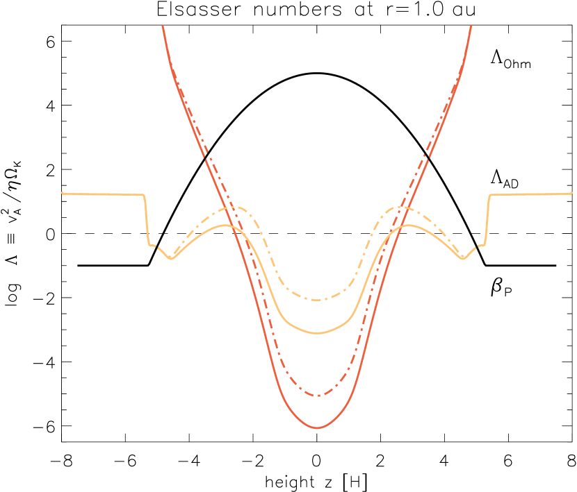
Figure 1.— Profiles of the initial Elsasser numbers (at radius $r=1\,\rm au$) for ohmic resistivity (light orange), and ambipolar diffusion (red). Solid lines represent the fiducial case of a dust-to-gas mass ratio of $10^{-3}$, whereas dash-dotted lines show profiles for a value of $10^{-4}$. We also plot the initial profile of the plasma $\beta$ parameter (solid black line).

The resulting initial ionization profile expressed in Elsasser numbers $\Lambda_{\rm O/AD}\equiv v_{{\rm A}\,z}^{2}\,(\Omega\,\eta_{\rm O/AD})^{-1}$ with $v_{{\rm A}\,z}\equiv B_{z}/\!\sqrt{\rho}$ is plotted in Fig. 1 at a radius of $1\,\rm au$, together with the height-dependent plasma $\beta$ parameter. The implications of this figure for our simulations are discussed in Sect 3.1. The region with $|z|\,\hbox{\lower 1.50696pt\hbox{$\sim$}\hbox to0.0pt{\hss\raise 1.50696pt\hbox{$>$}}}\,5\,H$, where the plasma parameter becomes constant with height is caused by applying a lower limit on the gas density to avoid excessive Alfvén speeds in the disk halo. Following BS13, we chose this limit at $10^{-6}$ (in our global model, this value is with respect to the initial midplane value at any given cylindrical radius). We remark that the equilibrium density profile is artificially steep in our isothermal disk model with temperature constant on cylinders. In this respect, the density floor acts to mimic a disk with realistic radiation thermodynamics, where the irradiation heating of the upper disk layers naturally creates an increased pressure scale height and hence a much shallower density profile. Because $\eta_{\rm AD}$ (and hence $\Lambda_{\rm AD}$) depends on the magnetization of the plasma, the actual density profile in the disk halo has an influence on how well the gas is coupled to the magnetic field lines, which in turn affects the efficiency of the magneto-centrifugal wind launching mechanism. This caveat should be kept in mind when interpreting the mass loading of the wind, which we expect to be a function of the thermodynamics in real protoplanetary disks.

2.2. Global disk model

We now describe the underlying protostellar disk model, which is largely identical to the one used in Gressel et al. (2013). The equilibrium disk model is based on a locally-isothermal temperature, $T$, decreasing with cylindrical radius as $T(R)=T_{0}\,(R/R_{0})^{q}$. For $q=-1$, such a profile leads to a constant opening angle throughout the disk as it is commonly used for global numerical simulations of PPDs, and which provides us with the reference disk model here. To study what effect disk flaring has on the absorption of direct FUV photons, we also produce a moderately flaring disk with $q=-3/4$. For this value, the resulting power-law index for the local opening angle, $h(R)\equiv H(R)/R$, is $\psi\equiv(q+1)/2=0.125$, which is in agreement with observational constraints for this value based on sub-mm observations (Andrews et al., 2009), and from multi-wavelength imaging (Pinte et al., 2008). The radial power-law exponents for the gas surface density, $\Sigma(R)$, are $-1/2$ for our fiducial model, and $-3/8$ for the flaring disk model, respectively.

Our temperature distribution is complemented by a power-law for the midplane density, $\rho_{\rm mid}(R)=\rho_{0}\,(R/R_{0})^{p}$, with $p=-3/2$. The equilibrium disk solution is given by

$$\rho(\mathbf{r})=\rho_{0}\left(\frac{R}{R_{0}}\right)^{p}\exp{\left(\,\frac{G\,M_{\odot}}{c_{\rm s}^{2}}\left[\frac{1}{r}-\frac{1}{R}\right]\,\right)}\,,\;\textrm{and}\quad$$ (5)

$$\Omega(\mathbf{r})=\Omega_{\rm K}(R)\,\left[\,(p+q)\left(\frac{H}{R}\right)^{\!\!2}\!+(1+q)-\frac{qR}{r}\,\right]^{\frac{1}{2}}\!\!,$$ (6)

which can be derived from the requirement of hydrostatic/-dynamic force balance in the vertical and radial directions, and where the Keplerian angular velocity $\Omega_{\rm K}(R)=\sqrt{G\,M_{\odot}}\,R^{-3/2}$. In the above equations, the square of the isothermal sound speed results from the prescribed temperature profile as $c_{\rm s}^{2}=c_{\rm s0}^{2}\,(R/R_{0})^{q}$, with a parameter $c_{\rm s0}$ corresponding to a value of $H(R)\equiv c_{\rm s}\Omega_{\rm K}^{-1}=0.05R$.

Guided by previous results of local 3D simulations that exhibit quasi-axisymmetric structure, we mainly focus on 2D-axisymmetric simulations. Our computational domain covers $r\in[0.5,5.5]\,\rm au$. In the latitudinal direction, the grid covers eight pressure scale heights on each side of the disk midplane, that is, $\theta\in[\pi/2-\vartheta,\pi/2+\vartheta]$, with $\vartheta=8\,H/r$. In the case of the flaring disk, the coverage of scale heights varies from $8\,H$ at $r=1\,\rm au$ to $6.5\,H$ at $r=5\,\rm au$. The grid resolution is $N_{r}\times N_{\theta}\times N_{\phi}=512\times 192\times 64$, which means that we are able to resolve relevant MRI wave lengths. In the axisymmetric models we use $N_{r}\times N_{\theta}=1024\times 384$ cells, corresponding to $\geq 24$ grid points per pressure scale height, matching the resolution of the three-dimensional box simulations of BS13. For the two non-axisymmetric simulations, the azimuthal extent is restricted to $\phi\in[0,\varphi]$, with $\varphi=\pi/2$ (a quarter wedge), or $\pi/4$ to limit the computational expense. We furthermore note that in the ideal-MHD case, where turbulence develops, the azimuthal domain size has been found to have an effect on the final saturated state(Beckwith et al., 2011; Flock et al., 2012; Sorathia et al., 2012), at least for the case of zero net flux.

Because our ionization model depends on real physical values of the gas column density, we have to chose a meaningful normalization factor $\rho_{0}$, which we fix according to a surface density of $\Sigma=150\,\rm g\,\rm cm^{-2}$ at the location $R=5\,\rm au$, compatible with the typical minimum-mass solar nebula (MMNS Hayashi, 1981). In physical units, the disk temperature is $T=540\,\rm K$ at a radius of $R=1\,\rm au$, and $T=108\,\rm K$ at $5\,\rm au$, resembling typical expected conditions within the protosolar disk. While our values for $\rho$, $T$ and $\Sigma$ are similar to the MMSN values at $5\,\rm au$, our adoption of different values for the radial power-law indices means that these values are different at $1\,\rm au$ compared to those adopted by BS13.

Our model disk is initially threaded by a weak vertical magnetic field $B_{z}(R)$ corresponding to a midplane $\beta_{\rm p\,0}\equiv 2p/B^{2}=10^{5}$ independent of radius for our fiducial disk. To achieve this, the vertical magnetic flux has to vary as a power-law in radius, taking into account the radial distribution of the midplane gas pressure that itself depends on the density and temperature. In our disk model, the gas pressure, $p(R)$ decreases outward, implying that $B_{z}(R)$ falls off with radius, too. While such a configuration is generally expected when accounting for inward advection and outward diffusion of the embedded vertical flux (Okuzumi et al., 2014), our particular choice of keeping the relative field strength constant is of course arbitrary. To preserve the solenoidal constraint to machine accuracy, we compute the poloidal field components from a suitably defined vector potential $A_{\phi}(r,\theta)$. The initial disk model is perturbed with random white-noise fluctuations in the three velocity components. The rms amplitude of the perturbation is chosen at one percent of the local sound speed. We furthermore add a white-noise perturbation in the magnetic field with an rms amplitude of a few $\mu{\rm G}$, which is on the sub-percent level compared with the net-vertical field of typically a few ten $\,\rm mG$.

2.3. Boundary conditions

To complete the description of our numerical setup, we need to specify boundary conditions (BCs). For the fluid variables, we employ standard “outflow” conditions at the inner and outer radial domain edges, $r_{\rm in}$ and $r_{\rm out}$. This type is a combination of a zero-gradient condition in the case of $\,\hat{\bf n}\cdot\mathbf{v}(r_{\rm in},\theta)>0\,$ (where $\hat{\bf n}$ denotes the outward-pointing normal vector), and reflective BCs in the opposite case, thus preventing inflow of material from outside the domain. At the upper and lower boundaries (that is, in the $\theta$ direction), we furthermore balance the ghost zone values such that a hydrostatic equilibrium is obtained. This helps to control artificial jumps of the fluid variables adjacent to the domain boundary as they are frequently encountered with finite-volume schemes.

In contrast to our earlier global simulations of layered accretion disks subject to Ohmic resistivity and containing an embedded gas-giant planet (Gressel et al., 2013), we here make a different choice for the vertical magnetic-field boundary condition. Whereas we previously applied magnetic BCs of the perfect conductor type (that is, forcing the normal field component to zero and allowing non-zero parallel field), we here use pseudo vacuum conditions, conversely enforcing the perturbed parallel field to vanish at the surface and only allowing a perpendicular perturbed field. Note that we exclude the initial net-vertical field from the procedure such that only deviations from the background field are subject to the normal-field condition. The vertical flux threading the disk is thus preserved. Since the disk’s upper layers are magnetically dominated, and the Lorentz force acts to align the flow lines with the magnetic field, letting the field lines cross the domain boundary is of course a prerequisite for launching an outflow. While we realize that forcing the radial and azimuthal components of the perturbed field to vanish at the boundary may unduly restrict the magnetic topology of the emerging wind solution, we postpone the study of less-restrictive but more cumbersome boundaries to future work.

Unlike in a radially-periodic local shearing-box simulation, our global model is critically affected by the inner radial boundary condition. In a real protoplanetary disk, we can expect that alkali metals will be thermally ionized in this region, leading to the development of the MRI on timescales short compared with the orbital timescale at the inner domain boundary of our model. This poses the question how to best interface the MRI-turbulent inner disk with the magnetically decoupled midplane of the outer disk that we model. It is likely that MRI-generated fields can efficiently leak into the outer disk via magnetic diffusion. In a first attempt to account for the MRI-active inner disk, we gradually taper the diffusivity coefficients to zero within the inner $0.5\,\rm au$ of our disk model. Studying the inner edge of the dead zone will however require dedicated simulations (similar to the ones performed by Dzyurkevich et al., 2010) including this transition region.

3. Results

The main aim of our paper is to establish the laminar wind solutions that BS13 previously found in local shearing box simulations in the context of global disk simulations. In the interest of economic use of computational resources and to guarantee adequate numerical resolution of our global models, we primarily focus on 2D axisymmetric simulations, but have also run three-dimensional simulations to check for non-axisymmetric solutions. Since all our runs include a net-vertical flux, axisymmetry is warranted to obtain a reading on the development of the MRI. In cases where the solution proves laminar, axisymmetry is likely to produce a reasonably accurate picture. We address the possibility of non-axisymmetric secondary instabilities using a limited set of three-dimensional calculations, described in Section 3.8.

Table 1Summary of simulation runs.

Run label	Ohm	AD	$\beta_{\rm p\,0}$	d/g	$q$	Resol.
O-b6	$\circ$	$-$	$10^{6}$	$10^{-3}$	-1	$1024\!\times\!384$
OA-b5	$\circ$	$\circ$	$10^{5}$	$10^{-3}$	-1	$1024\!\times\!384$
OA-b6	$\circ$	$\circ$	$10^{6}$	$10^{-3}$	-1	$1024\!\times\!384$
OA-b7	$\circ$	$\circ$	$10^{7}$	$10^{-3}$	-1	$1024\!\times\!384$
OA-b5-d4	$\circ$	$\circ$	$10^{5}$	$10^{-4}$	-1	$1024\!\times\!384$
OA-b5-flr	$\circ$	$\circ$	$10^{5}$	$10^{-3}$	-3/4	$1024\!\times\!384$
OA-b5-flr-nx	$\circ$	$\circ$	$10^{5}$	$10^{-3}$	-3/4	$512\!\times\!192\!\times\!128$
OA-b5-nx	$\circ$	$\circ$	$10^{5}$	$10^{-3}$	-1	$512\!\times\!192\!\times\!64$

Models are labeled according to the included micro-physical effects (first two letters) and the strength of the net-vertical magnetic field (expressed in terms of the midplane value $\beta_{\rm p\,0}$, prefixed with the letter ‘b’). Further labels refer to the dust-to-gas mass ratio (‘d/g’, prefixed with the letter ‘d’), the power-law index, $q$, of the radial temperature profile (‘flr’ for “flaring”), and whether the azimuthal dimension is included (‘nx’ for “non-axisymmetric”).

The simulations conducted for this work are listed in Table 1, where we summarize key model parameters. We assume a fiducial dust-to-gas mass ratio of $10^{-3}$, that is, a depletion by a factor of ten compared to interstellar abundances. Starting from the classic layered PPD (model ‘O-b6’) including only Ohmic diffusivity, we compare this standard “dead-zone” disk with a corresponding model, ‘OA-b6’, additionally including the effects of ambipolar diffusion. Our fiducial reference model is ‘OA-b5’, with a midplane plasma parameter of $10^{5}$. In the presence of combined ambipolar diffusion and Ohmic resistivity, we observe the waning of the MRI, which is instead replaced by a laminar wind solution. Unlike in geometrically constrained shearing box simulations (BS13, Bai, 2013), we naturally obtain a field configuration with field lines bending outward on both “hemispheres” of the disk. Notably, this topology produces thin current layers, which have previously been discussed by BS13. The stability and evolution of these current layers will be one focus of our paper.

We perform additional analysis on the influence of further key input parameters. With the global disk model allowing direct illumination from the central star, it becomes possible to address the question of how the disk’s ionization is affected by disk flaring. This is studied in model ‘OA-b5-flr’, where we use a power-law index of $q=-3/4$ instead of $q=-1$ to obtain a moderately flaring disk surface as is supported by observations (Pinte et al., 2008; Andrews et al., 2009). The role of dust depletion, driven by processes such as coagulation into larger grains and/or sedimentation, is considered in model ‘OA-b5-d4’ with a reduced dust-to-gas mass fraction of $10^{-4}$ (as used in BS13) compared with our fiducial value of $10^{-3}$. For the sake of brevity, we here refrain from varying any of the many other input parameters of our model, as for instance, the X-ray or CR intensities, or the FUV penetration depth, as well as parameters affecting the disk thermodynamics.

3.1. Preliminaries

The inputs to our models are very similar to those included in BS13, so it is instructive to compare the Elsasser number profiles in our model with their fiducial model as a means of understanding the similarities and differences between their results and ours. The fiducial model presented in BS13 is computed at $1\,\rm au$, and has a dust-to-gas mass fraction of $10^{-4}$, so we can compare this with the dot-dashed lines in Figure 1. The profiles shown there, and in figure 1 of BS13 are similar, with $\beta_{\rm P}$ decreasing below unity at disk heights $|z|\gtrsim 4.5H$, preventing MRI turbulence from developing at these high altitudes. In their initial condition and ours, $\Lambda_{\rm O}$ increases monotonically from the midplane upward. The two initial states also have similar profiles for $\Lambda_{\rm AD}$, displaying local maxima at intermediate disk heights ($z\sim\pm 2.5H$). The differences in the surface densities in the BS13 models and ours at $1\,\rm au$, combined with our inclusion of a direct X-ray component in addition to the scattered component means that $\Lambda_{\rm AD}\sim 10$ at this local maximum in our model, whereas it only rises modestly above unity in BS13. We therefore expect that our model with a dust-to-gas mass fraction of $10^{-4}$ should contain narrow regions at intermediate heights that support the growth of MRI channel modes. It is noteworthy that BS13 also observed the development of the MRI at the beginning of their simulations, but report that the subsequent amplification of the field causes the ambipolar diffusion to increase. Their disk then relaxes to completely laminar state in which angular momentum transport is driven by a magneto-centrifugal wind. The larger value of $\Lambda_{\rm AD}$ in our models may allow MRI turbulence to be sustained in these regions, or may instead lead to quenching of the MRI after it has reached a more nonlinear stage of development. In this paper, we define our fiducial model to be one in which the dust-to-gas mass fraction is $10^{-3}$, and the Elsasser numbers for this case are shown by the solid lines in Fig. 1. The larger dust concentration reduces the gas-phase electron fraction and Elsasser numbers, and the local maximum in $\Lambda_{\rm AD}$ now peaks moderately above unity (but still attaining a larger peak value than the fiducial model in BS13).

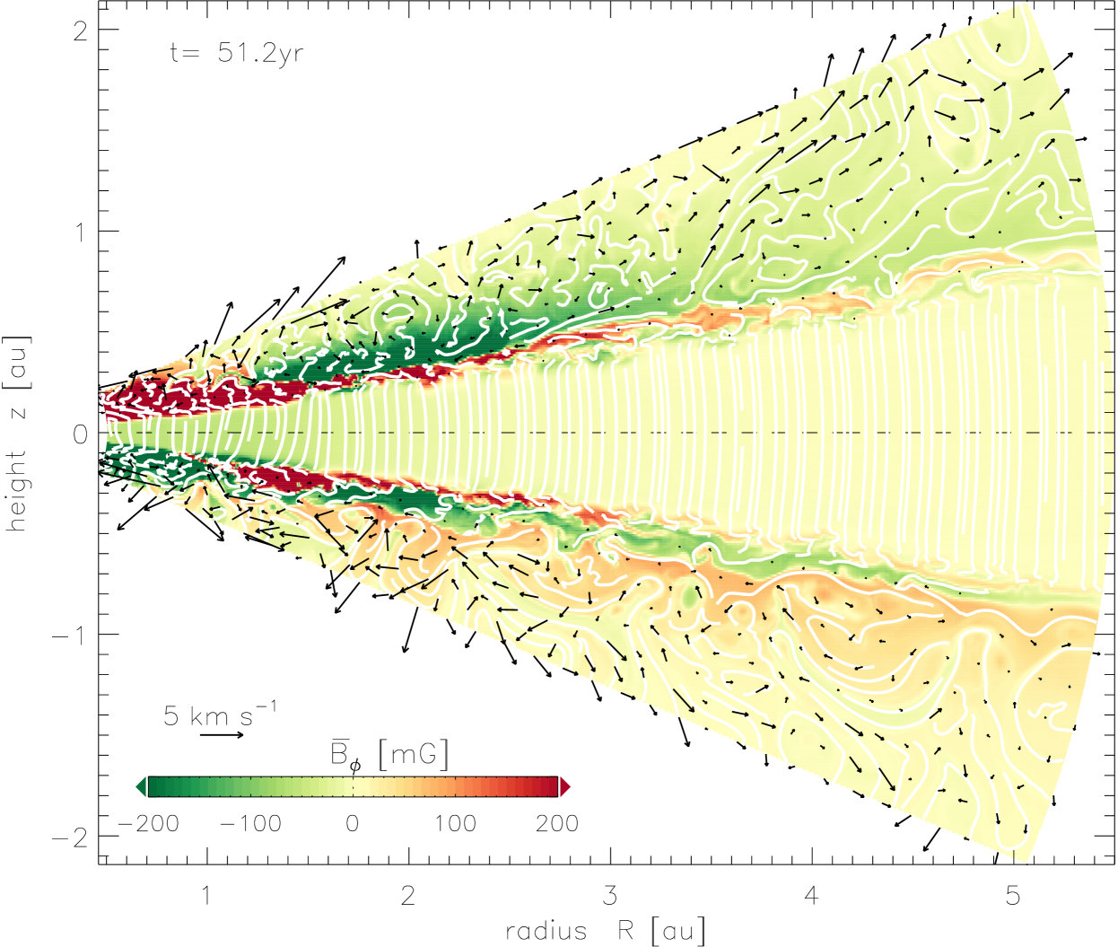
Figure 2.— Visualization of the global disk structure for model O-b6 with only Ohmic resistivity and $\beta_{\rm p\,0}=10^{6}$. The azimuthal fields reach peak strengths of $\simeq 2.5\,{\rm G}$ in the active disk layers. Vertical outflow is intermittent, but regions of an ordered wind geometry can be identified (see upper half around $3.5-4\,\rm au$).

3.2. Traditional dead zone model

We begin discussion of the simulation results by considering the 2D axisymmetric run O-b6, for which Ohmic resistivity is included and ambipolar diffusion is neglected. To introduce our setup, and give the reader an impression of the general appearance of our PPD model, Fig. 2 visualizes the magnetic field and poloidal flow vectors from the model. The color coding of the azimuthal field strength shows the MRI-turbulent surface layers with tangled poloidal field lines superimposed in white. In the outer disk, where the MRI has not fully developed yet, the parity of the horizontal field is odd with respect to reflection at the $z=0$ line, consistent with the winding-up of vertical field, $B_{z}$, by the weak differential rotation $\partial_{z}\,\Omega$ of our disk model. While the inner domain boundary also shows an odd field symmetry, intermediate sections of the disk show a mixed parity, reflecting the presence of MRI modes with both even and odd vertical wave numbers. Quite remarkably, the MRI channels extend over several AU in the radial direction, although we remark that this may be overly pronounced in the axisymmetric case, where the growth of parasitic modes is likely to be artificially restricted (Pessah & Chan, 2008). Because we use a net-vertical field, the linear MRI modes appear more pronounced than in the otherwise comparable 3D simulations of Dzyurkevich et al. (2010) without a net $B_{z}$ field.

The poloidal velocity field plotted as black arrows is mostly disordered in the turbulent regions but also shows some level of coherence in the upper layers, where a wind topology can be seen. While the wind is intermittent rather than steady and laminar, a general tendency for outflow is seen. This is consistent with similar observations of disk winds being launched from fully-MRI-active accretion disks (see, e.g., Suzuki & Inutsuka, 2009; Fromang et al., 2013). We quantify the mass loss via the vertical disk surfaces by evaluating

$$\dot{M}_{\rm wind}\equiv\left.2\pi\,\int_{r=r_{\rm i}}^{r_{\rm o}}\,\rho v_{\theta}\,r\,\sin\theta\,{\rm d}r\;\right|_{\theta=\theta_{1}}^{\theta_{2}}$$ (7)

at the upper and lower disk surface, $\theta=\theta_{1},\theta_{2}$, respectively. For model O-b6, we find a net mass loss rate of $\dot{M}_{\rm wind}=1.47\pm 0.37\times 10^{-8}\,M_{\odot}\,\rm yr^{-1}$ (also cf. Table 2 below).

We observe the formation of field arcs and material flowing downward along field lines towards the arc foot points. This can be seen in the lower disk half around $r=2.8\,\rm au$, and $r=4.3\,\rm au$, for example, and illustrates the potential role of buoyancy instability in regulating the disk’s magnetization. Amplification of the magnetic field through the growth of channel modes, and their break up through the action of parasites, apparently leads to the formation of these locally uprising field structures. As an alternative explanation, we remark that the dynamic evolution of such magnetic loops has previously been attributed to the effect of differential rotation onto the magnetic footpoints (Romanova et al., 1998).

In contrast, within the magnetically decoupled midplane layer, the magnetic field remains predominantly vertical, retaining the initial field configuration. Near the dead-zone edge, the effect of Ohmic diffusion gradually declines. There, the azimuthal magnetic field is allowed to change its value, resulting in localized current layers. This is very similar to the situation obtained in the disks that include ambipolar diffusion, as discussed later.

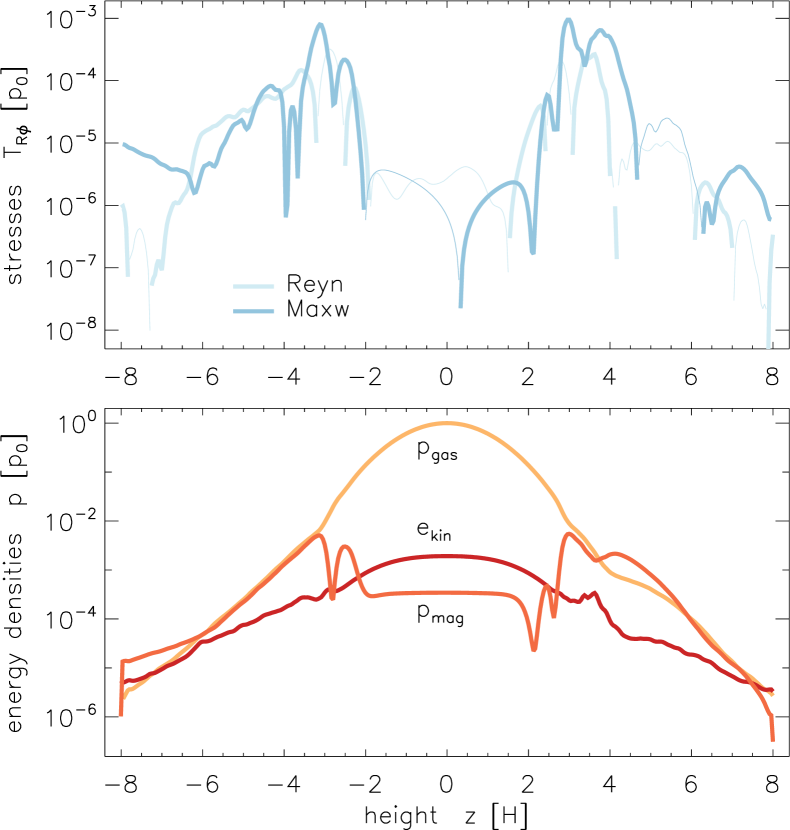
Figure 3.— Vertical profiles averaged over $r\in[2,3]\,\rm au$ and $t=25$ orbits for model O-b6 with Ohmic resistivity only and a midplane $\beta_{\rm p\,0}=10^{6}$. Negative values of the stresses (upper panel) are represented by thin lines.

We illustrate the vertical disk structure in Fig. 3, where we plot, in the upper panel, the total Reynolds and Maxwell stresses relative to the initial midplane gas pressure, $p_{0}$. The profiles show the typical signature of a laminar dead zone and MRI-turbulent surface layers (Fleming & Stone, 2003; Oishi et al., 2007; Gressel et al., 2011, 2012), where the mechanical and magnetic shear-stresses lead to transport of angular momentum. Because of the relatively weak net-vertical magnetic flux, the level of turbulence is modest, and the vertically-integrated dimensionless Maxwell stress is $\simeq 8\times 10^{-5}$. With the “viscous” mass accretion rate (i.e., that effected by internal stresses) approximated by

$$\dot{M}_{\rm visc}\approx\left.3\pi\,\Omega^{-1}\!\int_{\theta=\theta_{1}}^{\theta_{2}}\!\left(T_{R\phi}^{\rm Reyn}+T_{R\phi}^{\rm Maxw}\right)\,r\,{\rm d}\theta\;\right|_{r=r_{\rm ref}}\!\!,$$ (8)

we estimate a value of $\dot{M}_{\rm visc}\simeq 0.3\times 10^{-8}\,M_{\odot}\,\rm yr^{-1}$, at $r_{\rm ref}=2.5\,\rm au$, if mass accretion were effected by turbulent transport of angular momentum alone. This can be compared to the actual mass accretion rate, which we can easily compute in our global model via

$$\dot{M}_{\rm accr}\equiv\left.2\pi\,\int_{\theta=\theta_{1}}^{\theta_{2}}\,\rho v_{r}\,r^{2}\sin\theta\;{\rm d}\theta\;\right|_{r=r_{\rm ref}}\;.$$ (9)

Applying a radial average over $r\in[2,3]\,\rm au$, and estimating fluctuations occurring within a time interval spanning $t\in[75,100]\,\rm yr$, we find $\dot{M}_{\rm accr}=(0.14\pm 1.53)\times 10^{-8}\,M_{\odot}\,\rm yr^{-1}$ (also see the last column of Table 2). Clearly, this diagnostic turns out to be subject to strong fluctuations for model O-b6 – presumably due to the presence of strong radial motion within the MRI channel modes. Equation (9) will however prove useful when evaluating the radial drift of material in the localized current layers seen in the AD-dominated disk models. We note at this point that a simple energy conservation argument prevents the steady-state mass loss rate (to infinity) through a magneto-centrifugal wind being larger than the accretion rate through the disk. The large value of $\dot{M}_{\rm wind}$ reported above relative to $\dot{M}_{\rm accr}$ suggests that the wind loss rate is not yet converged. Indeed we note that BS13 report that increasing the vertical sizes of their shearing boxes leads to a reduction of the wind mass loss rates. A similar conclusion is reached by Fromang et al. (2013) for winds launched from turbulent disks. It appears that obtaining accurate and physically meaningful estimates for the mass fluxes through the upper boundaries of the disk will require simulations that are truly global in the vertical direction, such that the fast magnetosonic point is contained within the simulation domain rather than outside of the boundary as it is at present for all of the models that we present in this paper (ensuring that the wind launching region is causally disconnected from the imposed boundary conditions).

In the lower panel of Fig. 3, the gas pressure, kinetic energy and magnetic pressure, are shown. Within the dead-zone layer, between $z=\pm 4\,H$, the disk is supported by gas pressure alone, which follows a Gaussian profile. Owing to the additional magnetic pressure support within the active layer, the effective scale height increases roughly twofold there. Note that unlike seen in the isothermal simulations of BS13, cf. their fig. 3, the magnetic pressure does not significantly exceed the value of the gas pressure in large parts of the disk corona. We attribute this difference to the dissipation heating (Hirose & Turner, 2011) present in our simulations, which we note, however, may be overly pronounced in the axisymmetric models. The kinetic energy only becomes important very close to the vertical boundaries of our model. This is also reflected in the position of the Alfvén point, which is relatively poorly constrained and which we infer as $(7.60\pm 0.45)\,H$. Values for these vertical points are listed in Table 2 for all models. We report time- and space-averaged values obtained for $r\in[1,5]\,\rm au$, and we have appropriately taken into account the flaring of the disk. Because of the turbulent character of the upper disk layers, we cannot obtain a good estimate for the location of the base of the wind in model O-b6.

3.3. Laminar disk models with surface winds

We now discuss models that include both Ohmic resistivity and ambipolar diffusion. A key finding of BS13 is that the inclusion of ambipolar diffusion inhibits linear growth of the MRI in the intermediate disk layers, that is, the regions that are not affected by Ohmic resistivity. Since the ambipolar diffusion coefficient depends on the plasma parameter, one might expect that the effect of AD is less severe for high values of $\beta_{\rm p}$. To test this, we have run simulations OA-b6, and OA-b7, with $\beta_{\rm p\,0}=10^{6}$, and $10^{7}$, respectively.

3.3.1 Ambipolar diffusion with weak vertical fields

In accordance with the $\beta_{\rm p\,0}=\infty$ simulations of BS13, we find very low levels of turbulence in these simulations (cf. Table 2). As a consequence, the radial mass transport via accretion (see $\dot{M}_{\rm accr}$ values) is found to be negligible. At the same time, because of the weak vertical field, the magneto-centrifugal wind is absent in model OA-b7, and only poorly developed (and intermittent) in model OA-b6. We conclude that the corresponding field amplitude of about $10\,\rm mG$ (at $1\,\rm au$) can be assumed as a minimal requirement for significant mass transport by magnetic effects. In the following, we accordingly focus on models derived from our fiducial run OA-b5, with $\beta_{\rm p\,0}=10^{5}$, that is, $B_{z\,0}=31.5\,\rm mG$ ($4.2\,\rm mG$) at $1\,\rm au$ ($5\,\rm au$).

3.3.2 The fiducial model

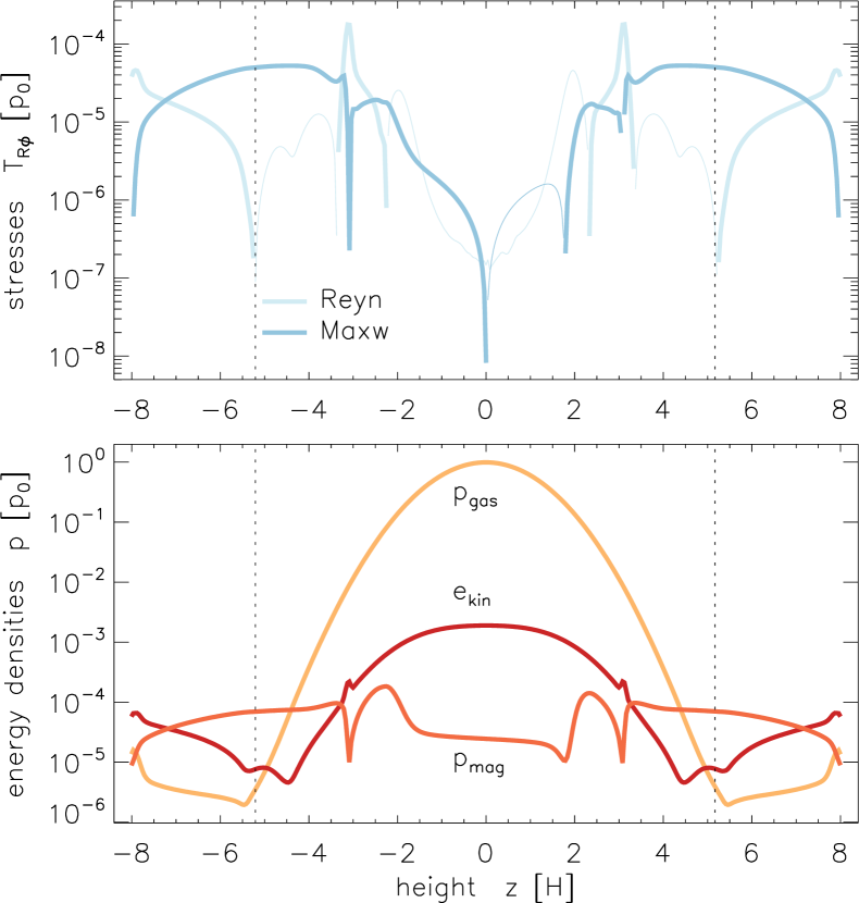
Figure 4.— Same as Fig. 3, but for model OA-b5 including both Ohmic resistivity and ambipolar diffusion, and with a stronger net-vertical field. Note the different scale of the abscissa in the upper panel, reflecting the reduced level of “viscous” transport. Dotted lines indicate the wind base at $z=\pm z_{\rm b}$.

In Figure 4, we show vertical profiles of the $R\phi$ stress components for our fiducial model, OA-b5, where owing to the stronger net vertical field the MRI is ultimately suppressed by ambipolar diffusion and a laminar wind solution is established instead. Dashed vertical lines indicate the base of the wind, which we define according to Wardle & Königl (1993) as the vertical position, $z=z_{\rm b}$, where the rotation becomes super-Keplerian. Since we define our azimuthal velocity, $v_{\phi}$ as the deviation from the Keplerian background flow, this can be verified in Fig. 4 by the fact that the Reynolds stress, $T_{R\phi}^{\rm Reyn}\equiv\rho\,v_{R}\,v_{\phi}$, vanishes at this point. The same is true for the vertical tensor component, $T_{z\phi}^{\rm Reyn}$, which makes it convenient to define the wind stress,

$$T_{z\phi}\equiv\left.T_{z\phi}^{\rm Maxw}\,\right|_{z=+z_{\rm b}}-\left.T_{z\phi}^{\rm Maxw}\,\right|_{z=-z_{\rm b}}$$ (10)

at this point. For the $R\phi$ component of the stress tensor, responsible for redistributing angular momentum radially, we furthermore obtain average values within the disk body $z\in[-z_{\rm b},+z_{\rm b}]$,

$$T_{R\phi}\equiv\frac{1}{2z_{\rm b}}\,\int_{-z_{\rm b}}^{+z_{\rm b}}\left(T_{R\phi}^{\rm Maxw}+T_{R\phi}^{\rm Reyn}\right)\,{\rm d}z\,,$$ (11)

which we list separately in Table 2, where values have been normalized to the midplane pressure, $p_{0}$. Already for a midplane plasma parameter as low as $10^{5}$, the wind stress exceeds the $R\phi$ (accretion) stress by a factor of four. BS13 also report that the wind stress exceeds the accretion stress; for their fiducial run, the discrepancy is bigger than an order of magnitude.

In the lower panel of Figure 4, we see that in the absence of MRI turbulence, the hydrostatic balance extends further up in the disk and the gas pressure remains the dominant stabilizing force all the way up to the base of the wind. Even in the magnetically dominated wind layer, magnetic pressure gradients remain moderate and the scale height of the disk remains roughly constant up to $z_{\rm b}$.

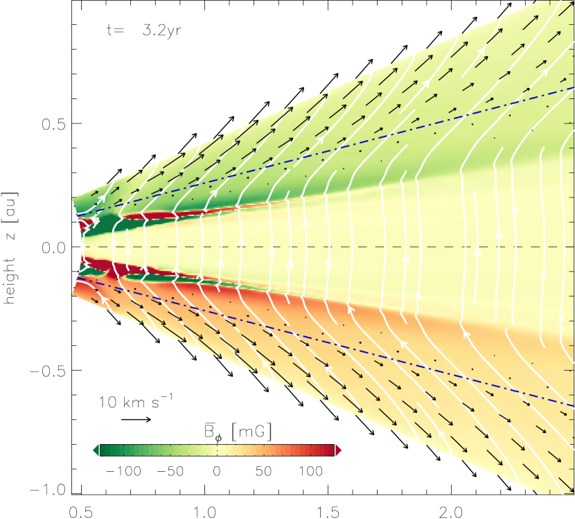
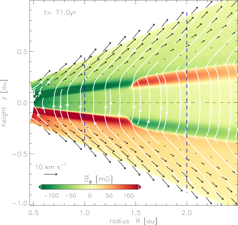
Figure 5.— Field topology of our fiducial simulation at different evolution times. The azimuthal magnetic field (color) has been restricted to values $|B_{\phi}|<125\,\rm mG$ for clarity; peak values are a few hundred ${\rm mG}$. We also show projected magnetic field lines (white) and velocity vectors (black). Additional lines indicate the position, $z_{\rm b}$, of the wind base (dot-dash), and the radial location of the profiles plotted in Figs. 6 and 7 (dashed lines).

In Fig. 5, we show a zoom-in of the inner part of the global field topology in our fiducial simulation OA-b5. The upper panel shows the resulting field configuration early on, when resistively modified MRI eigenmodes appearing inside $r=1.5\,\rm au$ are still clearly discernible. Localized channel solutions form at $z\approx 3\,H$ near the interface between the magnetically decoupled region, characterized by $\Lambda_{\rm O}\ll 1$ and purely vertical field lines with $B_{\phi}\approx 0$, and the AD-dominated intermediate layer. In this small region, both Elsasser numbers are above unity (cf. Fig. 1), allowing for linear growth of MRI channel modes. This transition layer is characterized by a zigzag-shaped abrupt change in the field lines (see Fig. 8 below), associated with strong current sheets. At this point, the laminar wind solution is already well established in the FUV ionized surface layer, and has spread throughout the radial extent of the simulation domain.

While the disk wind itself has already reached a steady state at this point in time, the strong field layers continue to evolve. In the lower panel of Fig. 5, we accordingly show a later evolution stage, where the relic MRI channels have morphed into strong azimuthal field belts. These field belts can be understood as “undead zones”, that is, a region that does not sustain MRI, but where diffusion can be balanced by the winding-up of preexisting radial field via differential rotation (Turner & Sano, 2008). It appears that the initial amplification of the magnetic field through the growth of channel modes causes the ambipolar diffusion coefficient to increase until it quenches further development of the MRI. This notion is supported by a reference simulation, where the diffusion coefficients $\eta_{\rm O}$ and $\eta_{\rm AD}$ were held fixed at their initial value, and where the MRI continues to produce quasi-turbulent fields akin to the ones seen in Fig. 2 for the Ohmic-only case. The reversal of the field direction seen at $r\simeq 1.5\,\rm au$ is a relic of the local nonlinear development of the MRI modes early on (as may be seen in the upper panel at $r\simeq 0.75\,\rm au$). This interface between the azimuthal field belts of opposite parity moves radially outward at a speed of $\approx 0.01\,\rm au\,\rm yr^{-1}$.

Table 2Summary of simulation results.

	$z_{\rm b}$	$z_{\rm A}$	$T_{R\phi}^{\rm Reyn}$	$T_{R\phi}^{\rm Maxw}$	$T_{z\phi}^{\rm Maxw}$	$\dot{M}_{\rm wind}$	$\dot{M}_{\rm accr}$
	$[H]$	$[H]$	$[10^{-6}p_{0}]$	$[10^{-5}p_{0}]$	$[10^{-5}p_{0}]$	$[10^{-8}\!\,M_{\odot}\!\,\rm yr^{-1}]$	$[10^{-8}\!\,M_{\odot}\!\,\rm yr^{-1}]$
O-b6	—	$7.60\pm 0.45$	$6.87\pm 14.4$	$7.44\pm 0.95$	—	$1.58\pm 0.59$	$0.04\pm 1.91$
OA-b5	$5.23\pm 0.07$	$7.31\pm 0.17$	$3.63\pm 0.19$	$2.22\pm 0.06$	$9.82\pm 0.08$	$0.79\pm 0.01$	$0.43\pm 0.01$
OA-b6	$7.22\pm 0.48$	$6.94\pm 0.37$	$\!\!\!-0.21\pm 0.18$	$0.79\pm 0.06$	$0.58\pm 0.06$	$0.19\pm 0.06$	$0.09\pm 0.02$
OA-b7	$7.31\pm 0.70$	$6.39\pm 0.16$	$0.07\pm 0.13$	$<0.01$	$0.22\pm 0.01$	$0.03\pm 0.01$	$0.00\pm 0.03$
OA-b5-d4	$5.27\pm 0.07$	$7.33\pm 0.18$	$0.11\pm 0.30$	$2.88\pm 0.11$	$9.88\pm 0.12$	$0.76\pm 0.02$	$0.34\pm 0.04$
OA-b5-flr	$4.81\pm 0.03$	$6.90\pm 0.31$	$0.26\pm 0.21$	$1.78\pm 0.02$	$14.3\pm 0.02$	$1.57\pm 0.01$	$0.64\pm 0.02$
OA-b5-flr-nx	$4.78\pm 0.03$	$7.50\pm 0.30$	$2.28\pm 9.24$	$1.87\pm 0.04$	$13.0\pm 0.04$	$1.58\pm 0.01$	$0.64\pm 0.03$
OA-b5-nx	$5.10\pm 0.04$	$7.34\pm 0.13$	$0.94\pm 9.29$	$1.89\pm 0.06$	$7.84\pm 0.02$	$0.67\pm 0.01$	$0.30\pm 0.04$

The vertical position of the base of the wind, $z_{\rm b}$, and the Alfvén point, $z_{\rm A}$, are found independent on the radial location when measured in local scale heights, $H$. The viscous accretion stresses $T_{R\phi}$ are vertically integrated within $|z|\leq z_{\rm b}$ – note the different units for Reynolds and Maxwell stresses. The wind stress, $T_{z\phi}$, is measured at $z=\pm z_{\rm b}$. All stresses depend weakly on radius; listed values are at $r=3\,\rm au$.

The emerging current layers are directly related to resistively-modified vertically-global MRI channel modes – see Latter et al. (2010), and Fig. 8 in Section 3.5. With MRI channels potentially spanning large radial extents, as in the Ohmic run shown in Fig. 2, such layers may be fed diffusively with magnetic field from the MRI-active inner disk. This is supported by our present models, where current layers appear to emerge from inner disk regions. What determines the exact shape of the surviving field configuration at late times is presently unclear. We speculate that the particular realization seen in the lower panel of Fig. 5 is not necessarily a unique solution given the specific disk geometry and ionization model, but may to some extend depend on the early evolution history. However, simulations that were initiated with different random seeds, but were otherwise identical, only showed minor variations in the final field appearance. The configurations observed at late times are moreover found to remain quasi-stationary, at least during the evolution time of $100\,\rm yr$ that we have investigated.

3.4. Typical wind solutions

Perhaps the most noteworthy result from run OA-b5 is the spontaneous emergence of the expected “hourglass” geometry for the magnetic field, allowing magnetic tension forces to accelerate the wind. For the adopted vertical field polarity, the field must bend radially outward near the upper and lower disk surfaces, and the azimuthal field should point in the positive direction in the lower hemisphere and reverse direction above the midplane, as observed in the upper panel of Figure 5.

3.4.1 Robustness of the emerging wind geometry

The shearing box simulations of BS13 have reflectional symmetry in the radial direction, that is, with respect to mirroring about $x=0$, and hence contain no information about the location of the star. Instead of giving rise to a physical wind solution, their fiducial run produces a radial field that possesses odd-symmetry about the midplane, with an inward pointing field in one hemisphere and an outward pointing one in the other. To test the robustness of the emerging solution in our setup, we initiate several instances of run OA-b5, using different random number seeds when perturbing the initial velocity field, and in each case we recover the correct wind solution with outward bending field lines. Our initial model has a net-vertical field with a radial dependence such that the midplane value of $\beta_{\rm p}$ remains constant. Because the gas pressure itself decreases with radius, the corresponding $B_{z}(R)$ (with $\partial_{R}B_{z}<0$) results in an outward magnetic pressure force, which moreover has a stronger acceleration effect in the low-density upper disk layers. While a vertical flux distribution that has the flux centrally concentrated can be expected when accounting for inward advection and outward diffusion of flux (Okuzumi et al., 2014), our particular choice is of course arbitrary. Radial magnetic gradients are furthermore known to affect the outflow’s mass loading in axisymmetric calculations where the disk is a boundary condition (Pudritz et al., 2006).

In our simulations, the pressure gradient related to $B_{z}(R)$ may potentially affect the direction toward which the field lines first bend from their starting configuration. We have tested this by running reference models with different magnetic pressure gradients. If $\partial_{R}B_{z}>0$, the initial condition has an unbalanced inward pressure force, and we do indeed find the field lines to spontaneously bend inward; this happens simultaneously in the upper and lower hemisphere of the disk, such that the overall symmetry that is obtained is again even. The launching of the inward wind is restricted to the inner disk, probably because the vertical field lines become too stiff (owing to $B_{z}$ increasing with radius) to be suitable for wind launching in the outer disk.

For a neutral situation with $\partial_{R}B_{z}=0$, we still observe outward bending of the field lines. Starting from the inner radial domain, the outward propagating establishment of the wind region is found to stall at some radius, whereas the wind was quickly established throughout the entire domain in model OA-b5. As before (for the case of an outward magnetic pressure gradient), this is probably related to the field lines becoming too strong to support the wind launching mechanism at large radii. The wind indeed stalls further out in a run with weaker overall net-vertical field. This poses the question whether the vertical profiles of $\Lambda_{\rm O}(z)$, and $\Lambda_{\rm AD}(z)$ that we obtain from our ionization model put strong constraints on permissible vertical field amplitudes as a requirement for wind launching.

A possible reason for the outward bending, even in the case of neutral magnetic pressure forces, may be that the vertical shear present in the global models (because of the baroclinic conditions) naturally bends the azimuthal component of the field in the correct direction required by the physical wind solution. We have checked that the outward bending of the vertical field lines is however equally seen in (strongly flaring) globally isothermal models that do not have any vertical gradients in the rotation velocity or any radial gradients in the vertical magnetic field. The outward pointing configuration is energetically favored because setting it up involves diluting rather than concentrating magnetic flux.

Our simulations demonstrate in any case that global models spontaneously develop the correct field geometry, although we caution that this conclusion needs to be tested in future simulations that moreover adopt improved boundary conditions for the magnetic field at the upper and lower (and potentially the inner radial) surfaces of the simulation domain. Ultimately, the emergence of the wind geometry will have to be studied in simulations that do not start from well-motivated (but nevertheless arbitrary) initial conditions, but do account for the formation of the PPD from a collapsing molecular cloud (Li et al., 2014).

Lastly, for the parameters that we have considered here, we do not find a self-limiting of the wind via shielding of FUV photons (Bans & Königl, 2012). This is consistent with the T Tauri scenario of Panoglou et al. (2012), who performed disk wind chemical modeling for various protostellar evolution stages. The authors find the shielding of FUV photons to be important for the Class I and Class 0 cases. Their T Tauri case, with mass flow rates comparable to our fiducial model, is sufficiently FUV-ionized to reduce ambipolar diffusion enough so that the neutrals are swept up in the wind out to at least a radius of $9\,\rm au$.

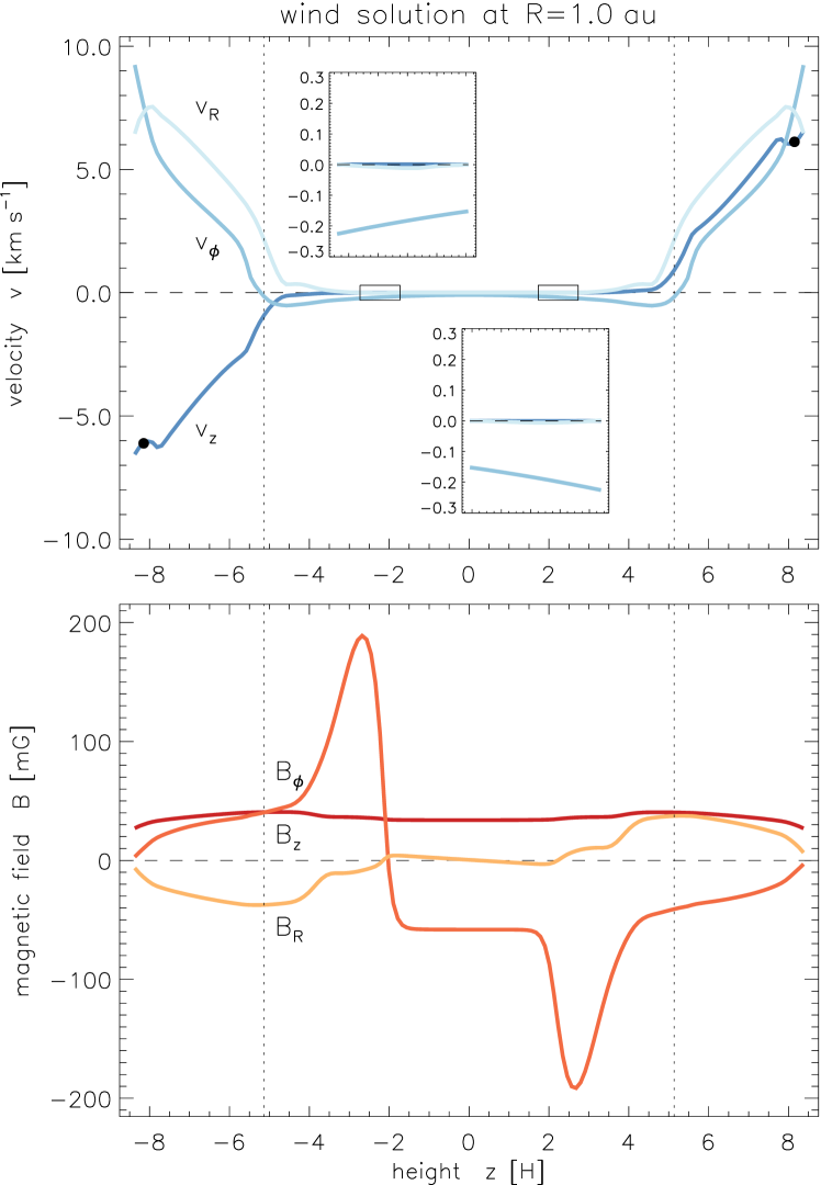
Figure 6.— Vertical profiles of the velocity components (upper panel) and the magnetic field components (lower panel) projected to cylindrical components for run OA-b5 at spherical radius $r=1\,\rm au$ (see the inner dashed line in Fig. 5b). The Alfvénic point with respect to $v_{\rm A\,z}\equiv B_{z}/\!\sqrt{\rho}$ is marked by filled circles. Dotted vertical lines indicate the base of the wind, defined as the point where $v_{\phi}$ becomes super-Keplerian (Wardle & Königl, 1993).

3.4.2 Comparison with local models

Except for the reversal of the horizontal magnetic field components (which at this stage appears to occur rather gently instead of within a narrow current layer), the field structure observed in the upper panel of Fig. 5 is similar to that described by BS13 and shown in their figure 10. Near the midplane, where the dominance of the Ohmic resistivity retards the growth of currents, the field is dominated by the vertical component. Moving to higher altitudes, where the magnetic coupling increases, the field bends outwards because a radial velocity is generated through the azimuthal force balance between the Coriolis force and magnetic tension. We enter the FUV layer at disk altitudes $|z|\gtrsim 4.5H$, coinciding with the base of the wind and the wind itself, as illustrated by the velocity vectors.

At later times, the lower panel of Fig. 5 shows that the varying polarity of the strong azimuthal field belts gives rise to two distinct field line geometries. In the inner region ($r\,\hbox{\lower 1.50696pt\hbox{$\sim$}\hbox to0.0pt{\hss\raise 1.50696pt\hbox{$<$}}}\,1.5\,\rm au$) the orientation of the field belts is the same as the one in the wind, and the vertical field lines bend smoothly at the transition into the wind base. Because some negative $B_{\phi}$ has diffused into the Ohmic-dominated midplane, there is a weak current layer forming at $z\simeq-2.15\,H$. In contrast, further out at $r\,\hbox{\lower 1.50696pt\hbox{$\sim$}\hbox to0.0pt{\hss\raise 1.50696pt\hbox{$>$}}}\,1.5\,\rm au$, the horizontal-field belts are anti-aligned with the magnetic field direction of the wind. This can also be seen in the curvature of the field lines, which are concave (towards the star) in this region. To connect the different layers, the azimuthal and radial field components have to change their direction within two thin current layers located at $z\simeq\pm 3.2\,H$. To study these configurations in more detail, we plot separate vertical profiles for $r=1\,\rm au$, and $r=2\,\rm au$ in Figs. 6 and 7, respectively. For easy reference, the radial positions are furthermore indicated in Fig. 5 by means of dashed lines. The isothermal sound speeds, for the initial disk model, are $c_{\rm s}=1.5\,\rm km\,s^{-1}$, and $1.1\,\rm km\,s^{-1}$ at the two respective radii.

The wind profile in the inner disk (see Fig. 6), is qualitatively similar to the wind solutions previously found in the quasi-1D simulations with “even-z” symmetry, plotted in fig. 10 of BS13. The current layer is much weaker in our case, and the dip in $v_{r}$ is barely visible in the left inset of Fig. 6. This may be related to differences in the ionization model resulting in $\Lambda_{\rm AD}>1$ in the region around $|z|\simeq 3\,H$, in our disk model. Differences in the particular diffusivity profiles also explain the pronounced peaks in $B_{\phi}$ in this “undead” transition layer, which are not seen in the simulations of BS13.

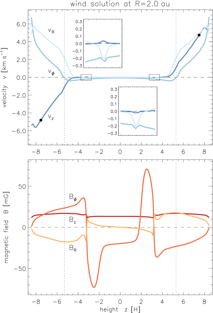
Figure 7.— Same as Fig. 6 but for $r=2\,\rm au$, where the horizontal field belts have opposite parity compared to the field within the wind layer. Inlays magnify the velocity profiles near the strong current layers, which reach a fair fraction of the local isothermal sound speed, $c_{\rm s}=1.1\,\rm km\,s^{-1}$.

The profile at $r=2\,\rm au$, with double field reversal in $B_{\phi}$, is illustrated in Fig. 7. Because of the strong current layers that are emerging in this case, this configuration resembles more closely the situation seen in the local models (again cf. fig. 10 in BS13). Unlike in their simulation, we however observe two current layers, one on each side of the disk. These arise because the development of MRI channel modes, and their subsequent evolution into “undead” azimuthal field belts with opposite polarity to the background wind, forces the horizontal field to change direction three times. Strong current layers occur at altitudes where the field and gas couple more strongly, namely at $|z|\sim 3H$. Although the occurrence of strong azimuthal field belts is not precluded in local simulations (as their existence may depend on the details of the ionization model), it seems likely that the alternating field belts we observe will only be a robust feature of global simulations. Apart from their multiplicity, the current layers appear very similar to the ones presented in BS13. The radial velocity $v_{r}$ shows a dip, while $v_{\phi}$ is modulated as a sine (the slight offset of $v_{\phi}$ in our simulation is due to the radial pressure support). The characteristic modulation (reflecting the abrupt kink in the field lines) is clearly seen in $B_{r}$ and $B_{\phi}$, which agree very closely with the $B_{x}$, and $B_{y}$ obtained by BS13. The emergence of such strong current layers naturally begs the question of their stability. Before we however discuss this issue in section 3.6, we first want to take a look at the current sheets’ likely origin as remnants of MRI eigenmodes.

3.5. Relation between current layers and channel modes

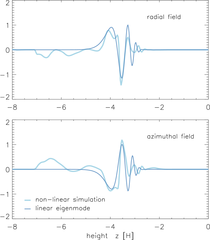
Figure 8.— Vertical structure of diffusively modified MRI channel modes, with Ohmic resistivity only. The solution that has been extracted from the nonlinear global simulation (light color) agrees markedly well with the linear eigenmode solution (dark color).

To draw a closer connection between localized MRI channel modes and the current layers observed in our simulations, we compare the structure of the fastest growing MRI eigenmode with the initial evolution of our standard setup with $\beta_{\rm p\,0}=10^{5}$. The mode structure we find is qualitatively similar to that shown for a spatially constant Ohmic resistivity (cf. the appendix of Fromang et al., 2013), and resembles the eigenmodes shown in figure 4 of Lesur et al. (2014), who performed Hall-MHD calculations that also included variable Ohmic resistivity. Dissipation modifies the MRI eigenmodes predominantly near the midplane, where the relative magnetization is lowest and the MRI wavenumbers are the highest, explaining the similarity of the solutions for constant $\eta$, and spatially varying $\eta=\eta(z)$.

Here, instead of a stratified shearing box framework as previously employed by Latter et al. (2010), we used the framework introduced by McNally & Pessah (2014) to capture the full vertical structure of the baroclinic initial condition. The eigenmode analysis uses the linear equations described in McNally & Pessah (2014, Section 5) with the addition of terms for spatially varying Ohmic resistivity, and using the functional forms and coefficients appropriate for the cylindrical temperature structure of the disk initial condition (McNally & Pessah, 2014, Section 3.3). The equations were discretized in real space with Chebyshev cardinal functions on a Gauss-Lobatto grid with 1000 points with the same vertical extent as the global simulation ($\pm 8$ scale heights). Boundary conditions were enforced by the “boundary bordering” method (Boyd, 2000) forcing the magnetic field perturbations to zero at the vertical edges of the domain. The analysis was performed at radial position $R=1\,\rm au$ where the Ohmic resistivity profile, $\eta_{\rm O}(z)$, used was extracted from the simulation initial condition and interpolated to the grid used for the eigenmode calculation.

We moreover obtained eigenmode solutions that additionally included a fixed $\eta_{\rm AD}(z)$ profile, and these showed a nearly indistinguishable mode structure. Because of the extra non-linearity introduced by the $\beta_{\rm p}$ dependence of $\eta_{\rm AD}(z)$, we however restrict our comparison to the Ohmic-only case. In Figure 8, we compare the early stage of our fully nonlinear global simulation with the fastest growing eigenmode. The localized field reversals are also clearly seen in the upper panel of Fig. 5, which shows the early evolution of model OA-b5 (however including AD). To isolate the linear MRI mode from the overlaid wind solution, we subtract respective field profiles from two distinct snapshots during the linear growth phase of the MRI. This is possible because the wind configuration emerges quickly, and then provides an approximately stationary background in which the MRI grows. Differencing two snapshots in time hence allows us to remove the wind part and extract the exponentially-growing MRI eigenmode. While growing perturbations near the midplane are high-wavenumber and thus efficiently damped, the relative field strength in the disk halo is too strong to allow for the MRI modes to fit within the available domain. This only leaves an intermediate disk region near $|z|\simeq 3.5\,H$ for MRI channel modes. In the Ohmic+AD simulations, this corresponds to the position of the “undead” field belts (see lower panel of Fig. 5) with adjacent current layers. In those simulations, the back-reaction of the growing eigenmodes on the $\eta_{\rm AD}(z)$ profile makes the MRI self-quenching, leaving the current layers as a remnant of the initial MRI channel mode.

3.6. Stability of current layers and horizontal field belts

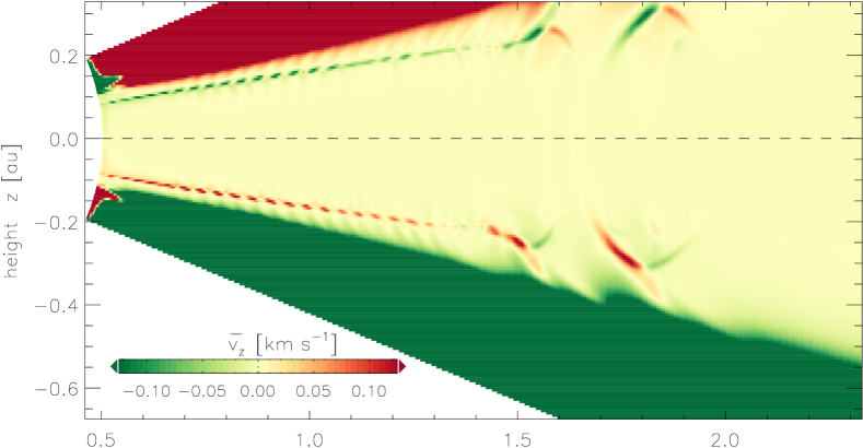
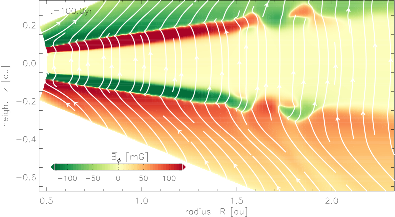
Figure 9.— Close-up showing the thin current layer of the flaring disk model OA-b5-flr breaking up into a KH-type instability. Top: vertical velocity, $v_{z}$. Bottom: azimuthal magnetic field strength, $B_{\phi}$, and poloidal magnetic field lines. The wavenumber of the perturbations is found to depend non-trivially on radius. Only for $r\,\hbox{\lower 1.50696pt\hbox{$\sim$}\hbox to0.0pt{\hss\raise 1.50696pt\hbox{$>$}}}\,1.5\,\rm au$, the nonlinear stage is clearly identified. The KH pattern is furthermore imprinted onto the mass-loading of the wind.

While we find the current layers to remain stable and long-lived in model OA-b5, some of the other simulations which we will discuss below also show signs of instability, leading to less regular fields.

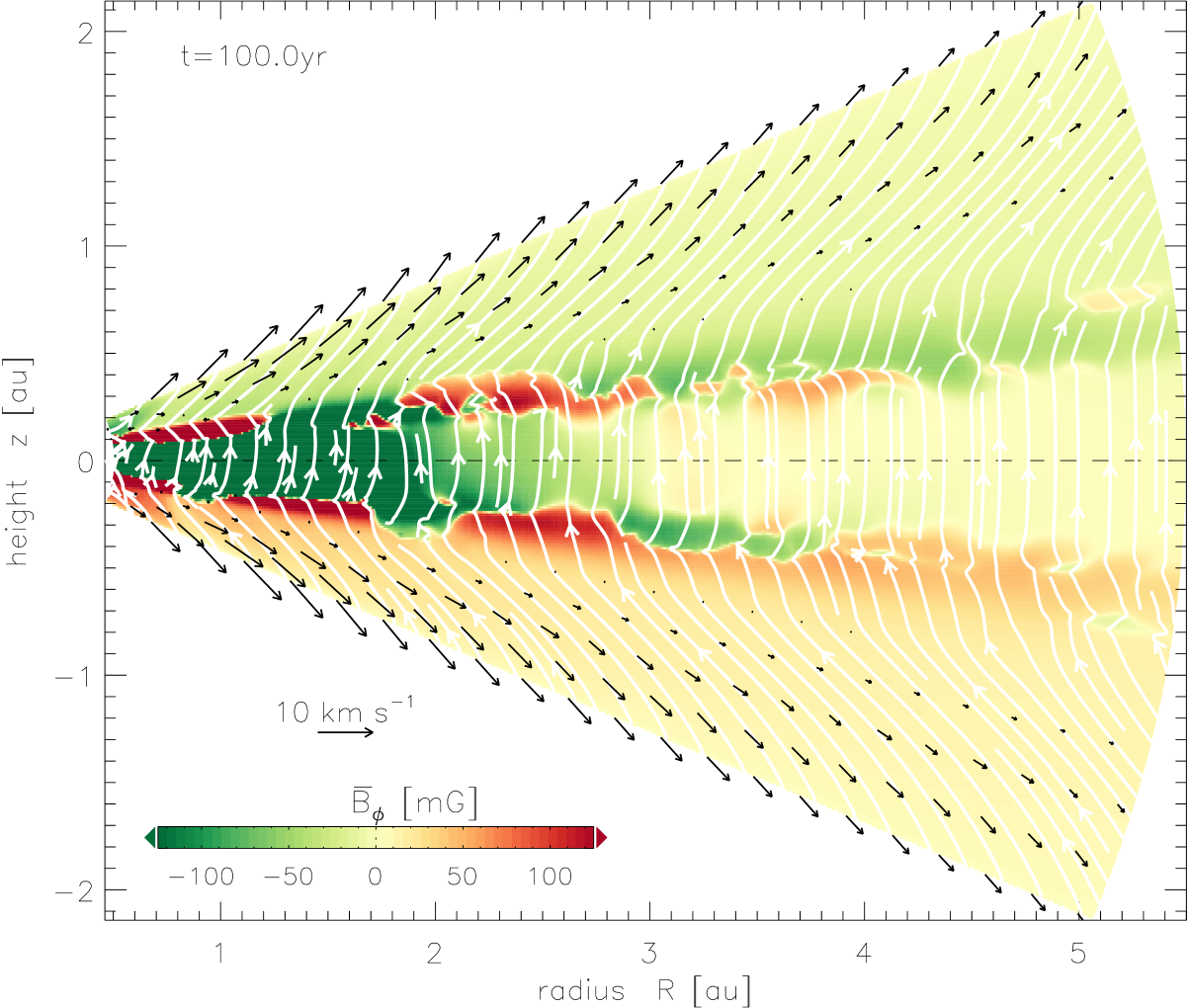
Figure 10.— Same as figure Fig. 5, but for model OA-b5-d4 with reduced dust fraction of $10^{-4}$, and showing the whole disk. Residual MRI fields form irregular patches below the wind layer leading to spatially intermittent current sheets.

3.6.1 Effect of disk flaring

An example of this is illustrated in Fig. 9, where we show the vertical velocity, $v_{z}$ (upper panel), and the azimuthal magnetic field, $B_{\phi}$ (lower panel), at the end of the flaring disk simulation OA-b5-flr. Both color scales have been restricted to highlight features in the current layer. In this model, the surface density interior to $1\,\rm au$ is smaller than in OA-b5, and beyond $1\,\rm au$ it is larger, altering the ionization structure sufficiently to put the current layer in a different regime. In particular, the increased ionization in the inner disk apparently allows the azimuthal field belts that form at intermediate heights to reach larger amplitudes. This, combined with the fact that these field belts are of opposite polarity relative to the background wind field, causes the two current layers located at $z\simeq\pm 3H$ to be stronger and to support narrow, radially directed flows, or “jets”, similar to those in run OA-b5, as illustrated in Figure 7.

Inside $r\simeq 1.4\,\rm au$, the velocity near the current layer shows a distinct radial wavenumber, suggesting that the shear associated with the radial jets leads to growth of a Kelvin-Helmholtz (KH) instability. The pattern, however, remains more or less stationary, indicating that the instability is not growing significantly into the nonlinear stage. Although not obvious in Fig.9, wave-like perturbations to the magnetic field are also present in the current layer. The possibility of current-driven tearing modes being present also arises, but analysis of the shear rate associated with the radial jets suggests that the observed instability is driven by KH modes. The velocity associated with the shear is super-Alfvénic, and is therefore expected to stabilize the tearing modes that may in principle grow in a shearing background (Chen et al., 1997).

The wavelength of the velocity perturbations and magnetic field changes abruptly for $r\,\hbox{\lower 1.50696pt\hbox{$\sim$}\hbox to0.0pt{\hss\raise 1.50696pt\hbox{$>$}}}\,1.4\,\rm au$, where now a characteristic vortex-pair pattern emerges. The exact reason for this abrupt transition is unclear, since most characteristic quantities, such as the Elsasser numbers $\Lambda_{\rm O}$, and $\Lambda_{\rm AD}$, only depend weakly and continuously on radius. The most likely explanation may be the radial variation of the azimuthal field (inside the “undead” belts), which drops in strength around this radial location. This is accompanied by a weakening and widening of the current layer, and a significant reduction in the inflow velocity of the radial accretion flow associated with the current layer, and a corresponding reduction in the shear relative to the background fluid. This suggests that the abrupt change in the nature of the disturbance observed at radius $\sim 1.8\,\rm au$ is unlikely to be driven by a KH instability, but the weakening of the shear may allow a tearing-mode instability to develop instead. The appearance of disturbances that have the character of growing magnetic islands provides some support for this interpretation, but this is clearly a tentative explanation that will require further investigation in future work. The presence of a background wind, Keplerian shear, ambipolar diffusion and a radially-directed inflow associated with the current layer make an analysis of this problem somewhat complicated, and beyond the scope of this paper. We note, however, that the local studies on the development of parasitic modes in resistive MHD (Latter et al., 2009; Pessah, 2010) may provide some insight, even though ambipolar diffusion is neglected in those studies. Pessah (2010) has analyzed MRI parasitic modes in the presence of finite Ohmic resistivity and viscosity. In this paper, $\Lambda_{\rm O}$, is identified as the relevant dimensionless number (see their figure 11), with tearing modes being the dominant parasitic modes for $\Lambda_{\rm O}\,\hbox{\lower 1.50696pt\hbox{$\sim$}\hbox to0.0pt{\hss\raise 1.50696pt\hbox{$<$}}}\,1$, and Kelvin-Helmholtz modes dominating otherwise. Considering both $\Lambda_{\rm O}$, and $\Lambda_{\rm AD}$, we assess that our simulations are situated near this transition point.

3.6.2 Effect of reduced dust fraction

Figure 10 shows the final appearance of the entire disk for model OA-b5-d4, which has a reduced dust fraction of $10^{-4}$ compared to a value of $10^{-3}$ in model OA-b5. On one hand, as the reader may check from Table 2, the two models are rather similar in their bulk properties, especially those related to the wind. This is unsurprising, since the reduced cross-section for recombination on grains affects the ionization fraction significantly only at large gas columns (see Fig. 1), below the base of the wind. The grains are less important for the ionization state in the FUV layer, where the electrons are so abundant that many remain free once the grains charge to the Coulomb limit (Okuzumi, 2009).

In contrast to our fiducial model, the transition between the base of the wind and the Ohmic-dominated disk interior is very chaotic in model OA-b5-d4, whereas it is much more stable in model OA-b5. It appears that the larger values of $\Lambda_{\rm O}$ and $\Lambda_{\rm AD}$ in this model at heights $z\sim\pm 2.5H$ allow the channel modes to grow further into the nonlinear regime, such that parasitic modes are able to develop and cause the field belts to break up into regions with locally coherent field. The field amplification during this phase means ambipolar diffusion strengthens, as in run OA-b5. Eventually the local evolution is driven by a combination of field winding and diffusion. The end result is the creation of local “undead” patches that evolve on timescales that are comparable to the run duration.

The different evolution of the horizontal field belts observed in runs OA-b5-flr and OA-b5-d4 compared with OA-b5 show that the evolution of the disk interior depends critically on the precise disk model that determines the Elsasser number profiles. In particular, the ionization state in the region between the Ohmic-dominated disk midplane and the AD-dominated intermediate disk layers depends sensitively on various model parameters. This suggests that a careful parameter study is required to obtain a reliable picture of how PPDs evolve over their life-times – especially since their properties change substantially over these time scales. Such a parameter study would appear to be most warranted when additional physics is included in the model, such as the Hall effect and more realistic thermodynamics. In a situation where the gas is allowed to be heated by resistive effects, the ionization balance may be shifted towards higher conductivity in the vicinity of the current layers, potentially leading to intermittent behavior (Faure, Fromang, & Latter, 2014; McNally, Hubbard, Yang, & Mac Low, 2014).

3.7. High-wavenumber instability at FUV transition

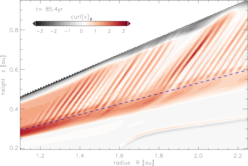
Figure 11.— Color-coded azimuthal component of the flow vorticity (at late time in model OA-b5), tracing high-frequency perturbations in the magnetically dominated disk corona. Perturbations originate at the base of the FUV layer (dashed line), and are aligned with the field lines of the wind solution.

A distinct instability emerges in the magnetically dominated corona of the laminar disk (see Fig. 11). The instability is found to grow close to the smallest available wavenumber, and is only present in the highly-resolved axisymmetric simulations. The perturbations are roughly aligned with the outward-pointing field lines of the laminar wind solution. Similar patterns have been observed in 2D-axisymmetric shearing box simulations with strong vertical fields performed by Moll (2012), who also finds field-aligned structures on the shortest length scales resolved on the grid. The instability also bears resemblance with the “striped wind” seen by Lesur, Ferreira, & Ogilvie (2013). Similar to the instability seen by Moll (2012), we find a moderate modulation of the vertical mass flux by the instability pattern. We however do not find material falling down along the field lines as reported there for certain parameters.

We identify three candidate mechanisms for creating such disturbances: (i) the vertical-shear instability investigated recently by Nelson, Gressel, & Umurhan (2013), potentially modified by anisotropy from field-line tension, (ii) a Kelvin-Helmholtz type instability related to the vertical gradient of the horizontal velocity near the base of the wind, and (iii) a buoyant interchange instability of the azimuthal field. It is important to note that the KH-type instability can create the elongated aspect ratio seen in Fig. 11, when perturbations are carried-away by the overlaid laminar wind velocity – and we indeed find this to be the case in situations where the instability occurred before the wind was established. The conclusive hint that a Kelvin-Helmholtz instability causes the pattern in Fig. 11 is a strong velocity gradient at the exact location of the transition into the FUV layer. This gradient can be clearly identified in Fig. 7 (situated just above the wind base at $z_{\rm b}$). The shear layer manifests itself as an additional steepening of the wind profiles, and can also be seen in the corresponding plot of BS13 (see their figure 10).

The physical origin of this sharp velocity gradient can be traced back to a peak in the ambipolar part of the electromotive force in the induction equation. Because the coefficient $\eta_{\rm AD}(r,\theta)$ sharply drops at the position of the FUV interface, the term $\nabla\times(\eta_{\rm AD}\,[\,(\nabla\!\times\!\mathbf{B})\times\hat{{\mathbf{b}}}\,]\times\hat{{\mathbf{b}}})$ can become significant in the induction equation even for smoothly varying (or constant) $\mathbf{B}$. In the steady state, this curl of the ambipolar electromotive force needs to be balanced by the induction term, $\nabla\times(\mathbf{v}\times\mathbf{B})$, requiring as a consequence a significant shear gradient in the horizontal velocity (again assuming a smooth $\mathbf{B}$). Given its strong dynamical effect, this raises the question whether the coincidence of the wind base and the FUV interface is in fact accidental as claimed by BS13.

In our disk model, the FUV layer is imposed ad hoc, with a prescribed column density (Section 2.1.1). The resulting interface is smeared out to a prescribed width. Reflecting the predominant direct origin of the FUV photons, while scattering is expected to remain negligible, the tapering is done in the radial direction, and as a function of column density (rather than position). As a consequence, the resulting $\eta_{\rm AD}(r,\theta)$ may develop sharp steps on the numerical grid in the $\theta$ direction – in turn resulting in sharp velocity gradients. We accordingly ran a reference model, where the FUV transition was softer. In this model, we did not observe a strong velocity gradient near the wind base, and also found the instability to be largely suppressed. Also the flaring-disk model, OA-b5-flr, did not show any signs of the instability. This can potentially be explained by the FUV transition following a concave line in this case, producing a different aliasing of the tapering function on the spherical-polar mesh. We conclude that the instability seen in Fig. 11 is likely caused by the particular numerical parametrization of the FUV layer in our model, and is entirely unrelated to the “striping” instability seen in Moll (2012) and Lesur et al. (2013). The instability may be be triggered by numerical effects at the grid scale, in a manner analogous to how physical secondary Kelvin-Helmholtz instabilities can be triggered by purely numerical effects as a shear layer thins to the grid scale (McNally et al., 2012). We remark that in the case of this wind instability too the mechanism behind the instability is genuinely physical, and may occur in real PPDs where there is a sharp local change in the ionization state.

3.8. Non-axisymmetric simulations

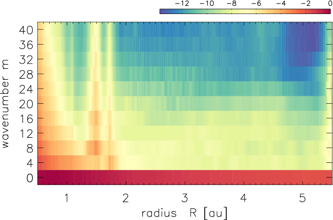
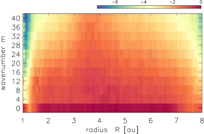
Figure 12.— Vertically-averaged azimuthal power spectra of the $B_{\theta}$ magnetic field. Top: Model OA-b5-flr with a laminar wind. Bottom: A run with MRI active surface layers in a domain of slightly different radial size, from Gressel et al. (2013). Owing to the restricted azimuthal extent in both runs, the only wavenumbers present are multiples of four.

The presence of secondary instability mandates investigating the non-axisymmetric evolution. This is done exemplarily for the two models OA-b5, and OA-b5-flr, whose 3D counterparts OA-b5-nx, and OA-b5-flr-nx are also listed in Table 2, showing only minor deviations from their respective 2D runs. Given the moderate magnetic Reynolds numbers in these regions, it is not per se obvious whether non-axisymmetric instabilities can transfer significant amounts of energy into modes with higher azimuthal wavenumber. To address this question, in Fig. 12, we show vertically-averaged azimuthal power spectra of the magnetic field. The color-coding indicates the logarithm of the power spectrum of $B_{\theta}$ as function of wavenumber, $m$, and radial position in the disk. In the upper panel, we show the result for model OA-b5-flr. With the exception of the Kelvin-Helmholtz features (between $R=1.5-2.0\,\rm au$) also seen in Fig. 9, almost all power resides in $m=0$. Even in the regions of the secondary instabilities, the power in modes with $m>0$ remains very small. The power seen adjacent to the inner radial domain boundary is caused by reducing the diffusion coefficients there, which is an attempt to mimic the MRI-active inner disk (see Section 2.3 for details).

This can be contrasted to the case of the classic layered PPD with MRI-active surface layers (see model M1 in Gressel et al., 2013), which we plot in the lower panel of Figure 12. Even with the laminar midplane layer, a significant amount of power is found for high-$m$ modes (note the different color bar in this figure). The lack of power near the radial boundaries is owing to a dissipative buffer region. Gressel et al. (2013) focused on the effects of a planet, which they inserted after the time shown here. We hence conclude that in the simulations that are dominated by axisymmetric configurations of AD-laminar winds, secondary instabilities do not lead to significant power in non-axisymmetric perturbations. This may potentially change in the presence of stronger current layers that are prone to nonlinear stage of parasitic modes as, for instance, can be seen for model OA-b5-d4 with a stronger dust depletion. When combined with stronger net-vertical fields and flaring, these dust-depleted disks may develop intermediate layers that are on the verge of becoming turbulent.

4. Summary

We have presented the first quasi-global MHD simulations of PPDs that include Ohmic resistivity and ambipolar diffusion. In agreement with the shearing box simulations of BS13, we find that the inclusion of ambipolar diffusion has a dramatic effect on the evolution. Our main results may be summarized as follows.

1. In simulations where we include a weak vertical magnetic field and Ohmic resistivity, but neglect ambipolar diffusion, we obtain evolution that is consistent with the traditional dead zone picture: surface layers that sustain MRI-driven turbulence and a quasi-laminar midplane region.

2. The inclusion of ambipolar diffusion in models with weak magnetic fields, where the midplane value of $\beta_{\rm P}>10^{5}$, results in quenching of the surface layer turbulence. Such disks display very weak internal motions and negligible angular momentum transport.

3. Our most important result arises when we increase the strength of the magnetic field so that $\beta_{\rm P}=10^{5}$. This leads to a disk which is entirely laminar between 1–$5\,\rm au$, and, despite the still relatively weak field, to the launching of a magnetocentrifugal wind from the upper ionized layers, resulting in a significant wind stress being exerted on the disk that drives inward mass flow at a rate $\gtrsim 10^{-8}\,M_{\odot}\,\rm yr^{-1}$.

4. We have tested the robustness of the wind solution by running multiple simulations with modified initial conditions. Because of the outward pressure force from the initial $B_{z}(R)$, and the vertical differential rotation, we generally obtain magnetic fields that point outwards in the radial direction in both hemispheres, as required for a physical wind solution that extracts angular momentum from the disk. This is with the exception of a model with $\partial_{R}B_{z}>0$, where an inward pointing wind was found.

5. The calculations treat the time-varying absorption of the FUV radiation from the star and its vicinity in the intervening material, yet there is no sign that absorption by the wind limits the ionization of the launching layer for mass loss rates in the T Tauri range.

6. Strong horizontal field belts are formed as remnants of stagnated MRI modes at intermediate heights in our disk models, and are likely maintained through a balance between field winding and ambipolar diffusion. These are found to have field polarities that may be aligned or anti-aligned with the background field associated with the wind, affecting the number of current layers that arise in the disk because of local field reversals. The belts polarity may depend sensitively on the early evolution of the MRI.

7. The current layers drive substantial accretion flows that are narrowly localized in height. The associated shear can be strong enough to allow small-scale Kelvin-Helmholtz instabilities to grow.

8. The global evolution of the horizontal field belts is found to depend on the Ohmic and ambipolar Elsasser numbers (and hence the ionization fraction). In our fiducial model, the belts alternate in polarity over large radial extents, but otherwise appear to be stable and only evolve on time scales that are long compared to the dynamical time scales.

9. Reducing the dust grain abundance by an order of magnitude, or allowing the disk to have a flaring structure, leads to more complex evolution in which the belts break-up into smaller-scale islands of locally coherent horizontal field polarity. We hypothesize that this evolution results from the increased ionization fraction that allows MRI channel modes to grow further into the nonlinear regime, where they are prone to break up via parasitic modes.

Our global simulations are most comparable to the shearing box simulations of BS13, and so it is worth briefly comparing our results with theirs. Our results for weakly magnetized disks ($\beta_{\rm P}>10^{5}$) with ambipolar diffusion and Ohmic resistivity compare well with their results for disks with no net vertical magnetic field, that is, no sustained wind and very weak turbulence and angular momentum transport. This indicates that there is a clear lower limit for the net vertical magnetic field required to drive an accretion flow that is in agreement with observations (given our restricted assumptions about the disk microphysics). Our results are in complete qualitative agreement with BS13 for higher magnetic field strength: disks are laminar and a magnetocentrifugal wind is launched from the highly ionized surface layers. The associated wind stress is sufficient to drive an accretion flow that matches typical rates measured to be reaching the surfaces of young stars.

Unlike earlier studies of magnetocentrifugal wind launching from deeper towards the midplane (Blandford & Payne, 1982; Pudritz & Norman, 1983; Wardle & Königl, 1993), there is no requirement for a strong magnetic field to be present in the disk when the wind is launched from high altitudes, since the requirements for field rigidity are met for globally weak fields in these low density regions. The appearance of long-lived horizontal field belts is not observed in the shearing box simulations of BS13, but this is because of modest differences in the disk models and assumed ionization physics (their model has a somewhat larger surface density at $1\,\rm au$, and we include a direct component to the disk illumination by stellar X-ray and FUV photons). The models agree qualitatively on the appearance of strong current layers, but the stability of these could not be examined by BS13 as their models in which the field geometry gave rise to these current layers used a quasi-1D approximation. This latter point illustrates the primary difference between the global and local shearing box simulations. The global simulations appear to produce and sustain the correct physical wind geometry spontaneously, whereas the symmetries associated with the shearing box normally lead to a radial magnetic field that points inwards in one hemisphere and outwards in the other, such that the correct geometry needs to be enforced. The potential role of the rather arbitrary initial conditions, and the vertical boundaries in setting the magnetic field topology in global models should be investigated. Our choice to impose a vertical field is motivated by the typical “hourglass” morphology (e.g. figures 2 and 3 in Kunz & Mouschovias, 2010, and references therein) emerging also in zoom-in simulations of PPD formation (Nordlund et al., 2014), and observed in molecular cores (Girart et al., 2006); even though the topologies of PPDs’ magnetic fields have not yet been unambiguously determined (Stephens et al., 2014; Davidson et al., 2014).

5. Conclusions

The results presented in this paper, combined with those by BS13, indicate that the traditional picture of a PPD hosting a dead zone in the shielded disk interior, with turbulent surface layers driven by the MRI, no longer holds. When ambipolar diffusion is treated, the flow becomes laminar, and accretion is driven by the magnetic stresses produced in launching a wind from the disk surface. Adding the Hall effect appears to further modify the flow by allowing a significant Maxwell stress to develop near the disk midplane through the combined action of field winding and Hall drift (Kunz, 2008; Kunz & Lesur, 2013; Lesur et al., 2014; Bai, 2014), but does not lead to turbulence. We are then left with a picture of PPDs in which the innermost regions sustain vigorous MRI-induced turbulence because of collisional ionization of alkali metals, the intermediate regions between $\sim 0.5-20\,\rm au$ are laminar with angular momentum transport occurring through a disk wind and perhaps through Maxwell stresses near the midplane (an effect that only arises if ${\bf\Omega}\cdot{\bf B}>0$ and when including the Hall term), and an outer region where the Hall effect and Ohmic resistivity are sub-dominant and weak turbulence arises (Simon et al., 2013; Bai, 2015).

The picture painted above has important implications for dust evolution and planet formation. In principle, dust coagulation and settling in the laminar region should occur rapidly, and in the absence of a source of stirring the loss of small grains should affect the spectral energy distribution (SED). This was examined by Dullemond & Dominik (2005), who showed that this rapid evolution of the SED is not in agreement with observations, and for many years this important result has provided indirect evidence for the existence of turbulent stirring in the planet forming regions of protoplanetary disks. In the absence of a magnetic origin for local turbulence this suggests that either another source of turbulence exists, such as the vertical shear instability (e.g. Nelson, Gressel, & Umurhan, 2013), or that small grains are continuously delivered to the laminar region from the outer and/or inner turbulent regions.

The results in this paper are consistent with the remanent magnetic field measurements in chondrules by Fu et al. (2014) in that the minimum midplane field strength for a wind driven disk at the presumed chondrule forming location (the midplane at $2$ to $3\,\rm au$) we find is smaller than the upper bound on the ambient field strength in the chondrule cooling region found in that work. This allows the chondrules studied by Fu et al. (2014) to have formed in the midplane of a wind driven laminar disk, while also allowing for the chondrule formation process to locally concentrate the magnetic field.

The influence of the traditional dead-zone picture for protoplanetary disks during various stages in planet formation has been examined in some detail. For example, Gressel, Nelson, & Turner (2011, 2012) showed that the stirring of planetesimals by the propagation of waves from the active region into the dead zone can stir up small planetesimals ($\lesssim 10\,\rm km$) and cause them to undergo collisional destruction, or prevent their runaway growth. In recent work (Nelson et al. 2014, in prep.), it has furthermore been shown that low mass planets orbiting in disk models with traditional dead zones are likely to undergo very rapid inward migration because the weak stresses there are unable to prevent saturation of the corotation torque. In principle, the new emerging picture of PPDs – that is, assuming that Maxwell stresses operate near the midplane because of the Hall effect – can ameliorate these problems by removing the turbulent stirring, and by providing a significant stress that can prevent corotation torque saturation. Full simulations are clearly required to examine whether or not the latter effect can be realized during full nonlinear evolution. Finally, Gressel et al. (2013) examined gap formation and gas accretion onto a giant planet within a disk with a traditional dead zone, and observed that the gas in the gap region became enlivened because of enhanced penetration of X-rays and cosmic rays. This created a turbulent and chaotic gas flow into the planet Hill sphere, and the enhanced magnetic coupling also led to the launching of a magnetocentrifugally accelerated jet from the circumplanetary disk. It remains unclear whether or not these effects will arise when ambipolar diffusion is included, given the low density of the gap region.

References

- Andrews et al. (2009) Andrews, S. M., Wilner, D. J., Hughes, A. M., Qi, C., & Dullemond, C. P. 2009, ApJ, 700, 1502
- Bai (2011) Bai, X.-N. 2011, ApJ, 739, 50
- Bai (2013) —. 2013, ApJ, 772, 96
- Bai (2014) —. 2014, ApJ, 791, 137
- Bai (2015) —. 2015, ApJ, 798, 84
- Bai & Goodman (2009) Bai, X.-N., & Goodman, J. 2009, ApJ, 701, 737
- Bai & Stone (2013) Bai, X.-N., & Stone, J. M. 2013, ApJ, 769, 76
- Balbus & Hawley (1991) Balbus, S. A., & Hawley, J. F. 1991, ApJ, 376, 214
- Balbus & Terquem (2001) Balbus, S. A., & Terquem, C. 2001, ApJ, 552, 235
- Bans & Königl (2012) Bans, A., & Königl, A. 2012, ApJ, 758, 100
- Baruteau et al. (2011) Baruteau, C., Fromang, S., Nelson, R. P., & Masset, F. 2011, A&A, 533, A84
- Beckwith et al. (2011) Beckwith, K., Armitage, P. J., & Simon, J. B. 2011, MNRAS, 416, 361
- Bethell & Bergin (2011) Bethell, T. J., & Bergin, E. A. 2011, ApJ, 739, 78
- Blaes & Balbus (1994) Blaes, O. M., & Balbus, S. A. 1994, ApJ, 421, 163
- Blandford & Payne (1982) Blandford, R. D., & Payne, D. G. 1982, MNRAS, 199, 883
- Boyd (2000) Boyd, J. P. 2000, Chebyshev and Fourier Spectral Methods, 2nd edn. (Dover, New York)
- Chen et al. (1997) Chen, Q., Otto, A., & Lee, L. C. 1997, J. Geophys. Res., 102, 151
- Choi et al. (2009) Choi, E., Kim, J., & Wiita, P. J. 2009, ApJS, 181, 413
- Cleeves et al. (2013) Cleeves, L. I., Adams, F. C., & Bergin, E. A. 2013, ApJ, 772, 5
- Davidson et al. (2014) Davidson, J. A., Li, Z.-Y., Hull, C. L. H., et al. 2014, The Astrophysical Journal, 797, 74
- Dullemond & Dominik (2005) Dullemond, C. P., & Dominik, C. 2005, A&A, 434, 971
- Dzyurkevich et al. (2010) Dzyurkevich, N., Flock, M., Turner, N. J., Klahr, H., & Henning, T. 2010, A&A, 515, A70
- Ercolano & Glassgold (2013) Ercolano, B., & Glassgold, A. E. 2013, MNRAS, 436, 3446
- Evans & Hawley (1988) Evans, C. R., & Hawley, J. F. 1988, ApJ, 332, 659
- Faure et al. (2014) Faure, J., Fromang, S., & Latter, H. 2014, A&A, 564, A22
- Fleming & Stone (2003) Fleming, T., & Stone, J. M. 2003, ApJ, 585, 908
- Flock et al. (2012) Flock, M., Dzyurkevich, N., Klahr, H., Turner, N., & Henning, T. 2012, ApJ, 744, 144
- Fromang et al. (2013) Fromang, S., Latter, H., Lesur, G., & Ogilvie, G. I. 2013, A&A, 552, A71
- Fu et al. (2014) Fu, R. S., Weiss, B. P., Lima, E. A., et al. 2014, Science, 346, 1089
- Gammie (1996) Gammie, C. F. 1996, ApJ, 457, 355
- Gardiner & Stone (2008) Gardiner, T. A., & Stone, J. M. 2008, JCoPh, 227, 4123
- Garmire et al. (2000) Garmire, G., Feigelson, E. D., Broos, P., et al. 2000, AJ, 120, 1426
- Girart et al. (2006) Girart, J. M., Rao, R., & Marrone, D. P. 2006, Science, 313, 812
- Gressel et al. (2011) Gressel, O., Nelson, R. P., & Turner, N. J. 2011, MNRAS, 415, 3291
- Gressel et al. (2012) —. 2012, MNRAS, 422, 1140
- Gressel et al. (2013) Gressel, O., Nelson, R. P., Turner, N. J., & Ziegler, U. 2013, ApJ, 779, 59
- Gullbring et al. (1998) Gullbring, E., Hartmann, L., Briceno, C., & Calvet, N. 1998, ApJ, 492, 323
- Hartmann et al. (1998) Hartmann, L., Calvet, N., Gullbring, E., & D’Alessio, P. 1998, ApJ, 495, 385
- Hawley & Balbus (1991) Hawley, J. F., & Balbus, S. A. 1991, ApJ, 376, 223
- Hawley et al. (1995) Hawley, J. F., Gammie, C. F., & Balbus, S. A. 1995, ApJ, 440, 742
- Hayashi (1981) Hayashi, C. 1981, Progress of Th. Phys. Suppl., 70, 35
- Hirose & Turner (2011) Hirose, S., & Turner, N. J. 2011, ApJ, 732, L30
- Hughes et al. (2011) Hughes, A. M., Wilner, D. J., Andrews, S. M., Qi, C., & Hogerheijde, M. R. 2011, ApJ, 727, 85
- Igea & Glassgold (1999) Igea, J., & Glassgold, A. E. 1999, ApJ, 518, 848
- Ilgner & Nelson (2006) Ilgner, M., & Nelson, R. P. 2006, A&A, 445, 205
- Kunz (2008) Kunz, M. W. 2008, MNRAS, 385, 1494
- Kunz & Lesur (2013) Kunz, M. W., & Lesur, G. 2013, MNRAS, 434, 2295
- Kunz & Mouschovias (2010) Kunz, M. W., & Mouschovias, T. C. 2010, MNRAS, 408, 322
- Landry et al. (2013) Landry, R., Dodson-Robinson, S. E., Turner, N. J., & Abram, G. 2013, ApJ, 771, 80
- Latter et al. (2010) Latter, H. N., Fromang, S., & Gressel, O. 2010, MNRAS, 406, 848
- Latter et al. (2009) Latter, H. N., Lesaffre, P., & Balbus, S. A. 2009, MNRAS, 394, 715
- Lesur et al. (2013) Lesur, G., Ferreira, J., & Ogilvie, G. I. 2013, A&A, 550, A61
- Lesur et al. (2014) Lesur, G., Kunz, M. W., & Fromang, S. 2014, A&A, 566, A56
- Li et al. (2014) Li, Z.-Y., Banerjee, R., Pudritz, R. E., et al. 2014, arXiv astro-ph:1401.2219
- McNally et al. (2014) McNally, C. P., Hubbard, A., Yang, C.-C., & Mac Low, M.-M. 2014, ApJ, 791, 62
- McNally et al. (2012) McNally, C. P., Lyra, W., & Passy, J.-C. 2012, ApJS, 201, 18
- McNally & Pessah (2014) McNally, C. P., & Pessah, M. E. 2014, ArXiv, astro-ph:1406:4864
- Meyer et al. (2012) Meyer, C. D., Balsara, D. S., & Aslam, T. D. 2012, MNRAS, 422, 2102
- Miyoshi & Kusano (2005) Miyoshi, T., & Kusano, K. 2005, JCoPh, 208, 315
- Mohanty et al. (2013) Mohanty, S., Ercolano, B., & Turner, N. J. 2013, ApJ, 764, 65
- Moll (2012) Moll, R. 2012, A&A, 548, A76
- Najita et al. (2009) Najita, J. R., Doppmann, G. W., Carr, J. S., Graham, J. R., & Eisner, J. A. 2009, ApJ, 691, 738
- Nelson & Gressel (2010) Nelson, R. P., & Gressel, O. 2010, MNRAS, 409, 639
- Nelson et al. (2013) Nelson, R. P., Gressel, O., & Umurhan, O. M. 2013, MNRAS, 435, 2610
- Nordlund et al. (2014) Nordlund, Å., Haugbølle, T., Küffmeier, M., Padoan, P., & Vasileiades, A. 2014, in IAU Symp., Vol. 299, IAU Symp., ed. M. Booth, B. C. Matthews, & J. R. Graham, 131–135
- Oishi et al. (2007) Oishi, J. S., Mac Low, M.-M., & Menou, K. 2007, ApJ, 670, 805
- Okuzumi (2009) Okuzumi, S. 2009, ApJ, 698, 1122
- Okuzumi et al. (2014) Okuzumi, S., Takeuchi, T., & Muto, T. 2014, ApJ, 785, 127
- Paardekooper et al. (2011) Paardekooper, S.-J., Baruteau, C., & Kley, W. 2011, MNRAS, 410, 293
- Panoglou et al. (2012) Panoglou, D., Cabrit, S., Pineau Des Forêts, G., et al. 2012, A&A, 538, A2
- Perez-Becker & Chiang (2011) Perez-Becker, D., & Chiang, E. 2011, ApJ, 735, 8
- Pessah (2010) Pessah, M. E. 2010, ApJ, 716, 1012
- Pessah & Chan (2008) Pessah, M. E., & Chan, C.-k. 2008, ApJ, 684, 498
- Pinte et al. (2008) Pinte, C., Padgett, D. L., Ménard, F., et al. 2008, A&A, 489, 633
- Pudritz & Norman (1983) Pudritz, R. E., & Norman, C. A. 1983, ApJ, 274, 677
- Pudritz et al. (2006) Pudritz, R. E., Rogers, C. S., & Ouyed, R. 2006, MNRAS, 365, 1131
- Romanova et al. (1998) Romanova, M. M., Ustyugova, G. V., Koldoba, A. V., Chechetkin, V. M., & Lovelace, R. V. E. 1998, ApJ, 500, 703
- Salmeron & Wardle (2003) Salmeron, R., & Wardle, M. 2003, MNRAS, 345, 992
- Salmeron & Wardle (2008) —. 2008, MNRAS, 388, 1223
- Sano et al. (2000) Sano, T., Miyama, S. M., Umebayashi, T., & Nakano, T. 2000, ApJ, 543, 486
- Sano & Stone (2002) Sano, T., & Stone, J. M. 2002, ApJ, 577, 534
- Sicilia-Aguilar et al. (2006) Sicilia-Aguilar, A., Hartmann, L., Calvet, N., et al. 2006, ApJ, 638, 897
- Simon et al. (2013) Simon, J. B., Bai, X.-N., Armitage, P. J., Stone, J. M., & Beckwith, K. 2013, ApJ, 775, 73
- Skinner & Ostriker (2010) Skinner, M. A., & Ostriker, E. C. 2010, ApJS, 188, 290
- Sorathia et al. (2012) Sorathia, K. A., Reynolds, C. S., Stone, J. M., & Beckwith, K. 2012, ApJ, 749, 189
- Stephens et al. (2014) Stephens, I. W., Looney, L. W., Kwon, W., et al. 2014, Nature, 514, 597
- Suzuki & Inutsuka (2009) Suzuki, T. K., & Inutsuka, S.-i. 2009, ApJ, 691, L49
- Turner et al. (2014) Turner, N. J., Fromang, S., Gammie, C., et al. 2014, ArXiv e-prints, arXiv:1401.7306
- Turner & Sano (2008) Turner, N. J., & Sano, T. 2008, ApJ, 679, L131
- Umebayashi & Nakano (1988) Umebayashi, T., & Nakano, T. 1988, Progress of Theoretical Physics Supplement, 96, 151
- Wardle (1999) Wardle, M. 1999, MNRAS, 307, 849
- Wardle & Königl (1993) Wardle, M., & Königl, A. 1993, ApJ, 410, 218
- Ziegler (2004) Ziegler, U. 2004, JCoPh, 196, 393
- Ziegler (2011) —. 2011, JCoPh, 230, 1035