Multi–dimensional Cosmological Radiative Transfer with a Variable Eddington Tensor Formalism

Abstract

We present a new approach to numerically model continuum radiative transfer based on the Optically Thin Variable Eddington Tensor (OTVET) approximation. Our method insures the exact conservation of the photon number and flux (in the explicit formulation) and automatically switches from the optically thick to the optically thin regime. It scales as $N\log N$ with the number of hydrodynamic resolution elements and is independent of the number of sources of ionizing radiation (i.e. works equally fast for an arbitrary source function).

We also describe an implementation of the algorithm in a Soften Lagrangian Hydrodynamic code (SLH) and a multi–frequency approach appropriate for hydrogen and helium continuum opacities. We present extensive tests of our method for single and multiple sources in homogeneous and inhomogeneous density distributions, as well as a realistic simulation of cosmological reionization.

1 Introduction

Numerous questions in physical cosmology and galaxy formation require a detailed understanding of the physics of radiative transfer. Of particular interest are problems related to the reionization of the intergalactic medium (Gnedin & Ostriker, 1997; Haiman et al., 2000; Barkana & Loeb, 2001, and references herein), absorption line signatures of high redshift structures (Abel & Mo, 1998; Kepner et al., 1999), and hydrodynamic and thermal effects of UV emitting central sources on galaxy formation (e.g. Haehnelt, 1995; Silk & Rees, 1998).

Several attempts have been made to develop numerical algorithms for solving the radiative transfer equation in astrophysics in general, and in cosmology in particular. Abel et al. (1999) described a ray tracing approach for modeling radiative transfer around point sources. A related ray tracing approach was introduced by Razoumov & Scott (1999) which can also handle diffuse radiation fields but finite computer memory limits the angular resolution and therefore only poorly captures ionization fronts around point sources on reasonably large grids. Ciardi et al. (2001) discussed a Monte Carlo approach to sample angles, energies and the time evolution of the radiative transfer problem. A ray tracing scheme for use with Smooth Particle Hydrodynamics was introduced by Kessel-Deynet & Burkert (2000). All these approaches however suffer from the excessive operation count and are costly to implement in realistic simulations Sokasian et al. (e.g. 2001).

In order to implement a radiative transfer scheme into modern numerical simulations, one needs to be able to solve the radiative transfer equation in $O(N)$ operations (where $N$ is the number of baryonic resolution elements, and we ignore a possible logarithmic multiplier, so that $O[N\log N]$ still counts as O[$N$]). However, the radiative transfer equation is six-dimensional in general and its direct solution requires of the order of $O(N^{5/3}\times N_{\nu})$ operations, where $N_{\nu}$ is the number of frequency bins (typically must be about 200-300). Various formal solutions of the transfer equation (like an attenuation equation) can be reduced to a four dimensional (spatial plus frequency dimensions) form, but then the calculation of the pairwise optical depth requires an operation count of the order of $O(N\times N_{S}\times N_{\nu})$, where $N_{S}$ is the number of sources, which for an arbitrary source function can be equal to $N$. For some restricted case, like reionization by quasars, when the number of sources $N_{S}$ is small enough, the whole solution can indeed be computed directly in $O(N)$ operations (Abel et al., 1999). However, for more realistic cases the operation count increases to $O(N^{2})$. In addition, in cosmological applications calculation of the background radiation field would still require $N^{5/3}$ operations.

Thus, one has to use approximations to try to decrease the operation count. The “Local Optical Depth” (LOD) approximation for the cosmological radiative transfer was first introduced in Gnedin & Ostriker (1997) for the homogeneous distribution of sources, and later was expanded on the case with an arbitrary source function in Gnedin (2000). This approximation is however highly approximate and uncontrolled.

Another possible approach is to use a so-called Variable Eddington Tensor approximation by solving moment equations for the radiative field. Such an approach allows to ensure exact conservation of photon numbers and flux, and thus would automatically give correct speeds for the ionization fronts. In this paper we describe such an approach whose main feature is the Variable Eddington Tensor approximation with the tensor calculated in the optically thin regime.

Norman et al. (1998) first suggested to solve the moment equations for the simulation of three dimensional radiative transfer in cosmological hydrodynamics. They suggested to split the transfer of radiation of point sources from the transfer of diffuse emitters. The method presented here shares some of their ideas, but works with different variables. We reformulate the equations of radiative transfer by decomposing the radiation field into a uniform component and a perturbation term. It is this new mathematical framework that we will present in the following section. In Section 3 we discuss our treatment of multiple frequency bins and also introduce a new “Reduced Speed of Light” approximation which allows us to overcome numerous numerical problems. We then go on in Section 4 to introduce particular details of our implementation of the algorithm. Section 5 is devoted to various one and three dimensional test cases that exemplify the strengths and weaknesses of our approach. We also present in that section a realistic cosmological simulation based on our new scheme, and compare our scheme with the LOD approach. We conclude in section 6 and give a discussion of various performance issues.

2 Formalism

2.1 Basic equations

The evolution of the specific intensity $J_{\nu}$ in the expanding universe is given by the following equation:

$${\partial J_{\nu}\over\partial t}+{\partial\over\partial x^{i}}\left(\dot{x}^{i}J_{\nu}\right)-H\left(\nu{\partial J_{\nu}\over\partial\nu}-3J_{\nu}\right)=-k_{\nu}J_{\nu}+S_{\nu}.$$ (1)

Here $x^{i}$ are the comoving coordinates, $H$ is the Hubble constant, $k_{\nu}$ is the absorption coefficient, $S_{\nu}$ is the source function, and $\dot{x}^{i}=cn^{i}/a$, where $n^{i}$ is the unit vector in the direction of photon propagation.

Equation (1) includes all relativistic effects and therefore is quite complex. But in the same spirit as equations for particle motions in the expanding universe are split into a uniform relativistic background and Newtonian perturbations, we can split equation (1) into a background and perturbations (Gnedin & Ostriker, 1997).

First, we define the mean specific intensity,

$$\bar{J}_{\nu}(t)\equiv\langle J_{\nu}(t,\vec{x},\vec{n})\rangle,$$ (2)

where the averaging operator $\langle\rangle$ acting on a function $f(\vec{x},\vec{n})$ of position and direction is defined as:

$$\langle f(\vec{x},\vec{n})\rangle=\lim_{V\rightarrow\infty}{1\over 4\pi V}\int_{V}d^{3}x\int d\Omega f(\vec{x},\vec{n}).$$ (3)

The mean specific intensity (“background”) satisfied the following equation:

$${\partial\bar{J}_{\nu}\over\partial t}-H\left(\nu{\partial\bar{J}_{\nu}\over\partial\nu}-3\bar{J}_{\nu}\right)=-\bar{k}_{\nu}\bar{J}_{\nu}+\bar{S}_{\nu},$$ (4)

where, by definition,

$$\bar{S}_{\nu}\equiv\langle S_{\nu}\rangle,$$

and

$$\bar{k}_{\nu}\equiv{\langle k_{\nu}J_{\nu}\rangle\over\bar{J}_{\nu}}.$$

It is important to emphasize here that we use the overbar symbol merely as a part of notation and not to denote the space average; in particular, $\bar{k}_{\nu}$ is not a space average of $k_{\nu}$ since it is weighted by the local value of the specific intensity $J_{\nu}$.

We can now introduce a new quantity, which we call relative (to the mean) specific intensity $f_{\nu}(t,\vec{x},\vec{n})$, which quantifies the difference between the local value of the specific intensity and the mean,

$$J_{\nu}\equiv f_{\nu}\bar{J}_{\nu},$$ (5)

so that $\langle f_{\nu}\rangle=1$. In the dynamic analogy, $f_{\nu}$ corresponds to $1+\delta$, where $\delta$ is the cosmic overdensity.

It is now straightforward to derive the following equation for $f_{\nu}$:

$${\partial f_{\nu}\over\partial t}+{\partial\over\partial x^{i}}\left(\dot{x}^{i}f_{\nu}\right)=H\nu{\partial f_{\nu}\over\partial\nu}-(k_{\nu}-\bar{k}_{\nu}+{\bar{S}_{\nu}\over\bar{J}_{\nu}})f_{\nu}+{S_{\nu}\over\bar{J}_{\nu}}.$$ (6)

This equation is of course not simpler than the original equation (1). But, if we restrict ourselves to scales significantly smaller than the horizon size, and matter velocities much smaller than the speed of light (Newtonian limit), then we can simplify equation (6) substantially by noting that the relative specific intensity does not change substantially and the universe does not expand substantially over the period of time a photon needs to travel over the scale under consideration (for example, a size of a computational box). Therefore, we can ignore the derivative with respect to the frequency. Strictly speaking, we should also discard the time derivative, as it has the same power of $v/c$ as the frequency derivative. However, we will retain it for a moment, keeping in mind that it is small - as we explain below, the time derivative turns out to be quite useful for the numerical implementation of our scheme.

Under these assumptions, equation (6) reduces to the following simple equation:

$${a\over c}{\partial f_{\nu}\over\partial t}+n^{i}{\partial f_{\nu}\over\partial x^{i}}=-\hat{\kappa}_{\nu}f_{\nu}+\psi_{\nu},$$ (7)

where

$$\kappa_{\nu}\equiv{a\over c}k_{\nu},$$

$$\hat{\kappa}_{\nu}\equiv\kappa_{\nu}-\bar{\kappa}_{\nu}+{\bar{S}_{\nu}\over\bar{J}_{\nu}}$$ (8)

and

$$\psi_{\nu}\equiv{a\over c}{S_{\nu}\over\bar{J}_{\nu}}.$$

Equations (4) and (7) thus separate the average cosmological evolution of specific intensity (including redshift and effects of “distant” sources - sources outside the simulation box) from the local evolution due to inhomogeneous absorption and sources inside the box.

2.2 Moments of the transfer equation

The transfer equation (7) is a six-dimensional equation in the phase space, and as such offers a considerable difficulty to solve numerically. Pursuing the analogy with dynamics further, we can define moments of the radiation field similarly to how density, momentum, pressure etc of a medium are defined as moments of the distribution function. Specifically, we define the (relative to the mean) radiation energy density $E_{\nu}$,

$$E_{\nu}(t,\vec{x})\equiv{1\over 4\pi}\int d\Omega\,f_{\nu}(t,\vec{x},\vec{n}),$$

the flux $F^{i}_{\nu}$,

$$F^{i}_{\nu}(t,\vec{x})\equiv{1\over 4\pi}\int d\Omega\,n^{i}f_{\nu}(t,\vec{x},\vec{n}),$$

and the so-called Eddington tensor $h^{ij}_{\nu}$,

$$E_{\nu}(t,\vec{x})h^{ij}_{\nu}(t,\vec{x})\equiv{1\over 4\pi}\int d\Omega\,n^{i}\vec{n}f_{\nu}(t,\vec{x},\vec{n}).$$

In particular,

$${\rm Tr\,}h^{ij}_{\nu}=1\ \ \ \mbox{and}\ \ \ \langle E_{\nu}\rangle=1.$$

Taking moments of equation (7), we can derive equations for the moments of the radiation field (assuming that the source function is isotropic):

$${a\over c}{\partial E_{\nu}\over\partial t}+{\partial F^{i}_{\nu}\over\partial x^{i}}=-\hat{\kappa}_{\nu}E_{\nu}+\psi_{\nu}$$ (9)

and

$${a\over c}{\partial F^{j}_{\nu}\over\partial t}+{\partial\over\partial x^{i}}E_{\nu}h^{ij}_{\nu}=-\hat{\kappa}_{\nu}F^{j}_{\nu}.$$ (10)

It is easy to see that equations (9) and (10) are in a conservative form, and so represent the conservation of the number of photons and the flux respectively.

Equations (9) and (10) constitute a system of two partial differential equations. The system is however not closed since the Eddington tensor is not specified by these two equations. However, if the Eddington tensor is given as a function of position and time, the system becomes closed. In the following section we assume that the Eddington tensor is known and describe the numerical implementation of an algorithm based on equations (9) and (10). We then discuss how to define the Eddington tensor, thus completing the numerical scheme.

3 Specific implementation

3.1 The “Reduced Speed of Light” approximation

In this section we omit the frequency dependence for clarity. Equations (9) and (10) can be combined into one equation preserving the accuracy of the Newtonian approximation. Namely, from (10) we have:

$$F^{j}=-{1\over\hat{\kappa}}\left({a\over c}{\partial F^{j}\over\partial t}+{\partial Eh^{ij}\over\partial x^{i}}\right).$$

Substituting this into (9), we obtain:

$${a\over c}{\partial E\over\partial t}+\hat{\kappa}E-\psi-{\partial\over\partial x^{j}}\left({1\over\hat{\kappa}}{\partial Eh^{ij}\over\partial x^{i}}\right)={a\over c}{\partial\over\partial x^{j}}\left({1\over\hat{\kappa}}{\partial F^{j}\over\partial t}\right).$$ (11)

The right hand side can be expanded into two terms,

$${a\over c}{\partial\over\partial x^{j}}\left({1\over\hat{\kappa}}{\partial F^{j}\over\partial t}\right)=-{a\hat{\kappa}_{,j}\over c\hat{\kappa}^{2}}{\partial F^{j}\over\partial t}+{a\over c\hat{\kappa}}{\partial\over\partial t}{\partial F^{j}\over\partial x^{j}}.$$

Both of these terms are of the order of $1/c$, and thus can be dropped in the Newtonian limit. We therefore neglect the first term, but retain the second one, keeping in mind that it is of the higher order in $1/c$ than the leading terms in equation (11). That leaves the right hand side of equation (11) in the following form:

$${a\over c\hat{\kappa}}{\partial\over\partial t}\left(-{a\over c}{\partial E\over\partial t}-\hat{\kappa}E+\psi\right),$$

of which we retain only one term,

$$-{a\over c}{\partial E\over\partial t},$$

with the same $1/c$ accuracy. This reduces the original equation (11) to the following final form:

$$2{a\over c}{\partial E\over\partial t}={\partial\over\partial x^{j}}\left({1\over\hat{\kappa}}{\partial Eh^{ij}\over\partial x^{i}}\right)-\hat{\kappa}E+\psi.$$ (12)

This one equation is equivalent to the original two equations (9) and (feq) in the Newtonian limit, and the term with the time derivative is small and formally of the order of $1/c$.

The physical reason for retaining the time derivative and throwing away other terms which are formally of the same order is that at the ionization front $E$ can change very rapidly making this term significantly larger than the terms we neglected, even if formally they have the same $1/c$ order.

In the Newtonian limit the speed of light is infinite, which in practice means that we ignore all the terms of the order of $v/c$. Thus, it actually does not matter what the specific value of the speed of light is as long as $v/c\ll 1$, and we can replace the true speed of light $c$ in equation (12) with some other quantity $\hat{c}$ without violating the validity of the Newtonian limit as long as $v/\hat{c}\ll 1$. For example, for modeling cosmological reionization we can adopt a value for $\hat{c}$ as low as $1,000\mbox{\,km}/\mbox{\,s}$, because typical gas velocities during reionization do not exceed $100\mbox{\,km}/\mbox{\,s}$.

This trick of “reducing the speed of light” (which we call the Reduced Speed of Light, or RSL, approximation) allows us to achieve a very important goal. Namely, if we ignore the time derivative term in equation (12), the equation turns elliptic, which is difficult to solve for an arbitrary $\hat{\kappa}$. Thus, keeping the time derivative in equation (12) allows us to solve this equation as a dynamical equation and use simple stable explicit schemes.

There is however one very serious limitation - the time-step in any explicit scheme will be limited by an appropriate Courant condition to a value which is about $c_{S}/c$ times smaller than the hydrodynamic time-step (here $c_{S}$ is the gas sound speed). For the intergalactic gas at $10,000\mbox{\,K}$ this ratio can be as small as $1/30,000$. Clearly, this will make such a scheme impractical, as it is impossible to make 30,000 radiative transfer time steps for every hydrodynamic time step in a realistic simulation.

The RSL approximation allows to reduce this ratio dramatically to less than 100, and in our tests described below we even find that taking $\hat{c}\sim c_{S}$ does not lead to large errors.

Thus, in the RSL approximation equation (11) reduces to the following form:

$$2{a\over\hat{c}}{\partial E\over\partial t}={\partial\over\partial x^{j}}\left({1\over\hat{\kappa}}{\partial Eh^{ij}\over\partial x^{i}}\right)-\hat{\kappa}E+\psi$$ (13)

where $\hat{c}\leq c$.

It is important to note here that the reduction in the speed of light does not limit the propagation speed of an ionization front to $\hat{c}$. Equation (13) is a diffusion equation, which has an infinite speed of signal propagation. In other words, the RSL approximation puts no limit on the speed of ionization fronts and thus can sometimes lead to unphysical, faster than the speed of light propagation of the ionization fronts (Abel et al., 1999). In practice, we put a limit on the maximum possible speed of an ionization front by limiting the number of time-steps. This is discussed in greater detail in §3.4.

3.2 Multi-frequency transfer

Equation (13) is a diffusion equation, and as such is not more difficult to solve than equations of hydrodynamics (in fact, it is much easier to solve). However, we have omitted the frequency dependence in the derivations of the previous section. Tests indicate that in order to calculate the various ionization and heating rates with sufficient precision on a logarithmically spaced mesh in frequency space, at least 20 points per e-folding are required, which translates into at least 200 frequency bins. Solving equation (13) 200 times at each hydrodynamic time step would be too prohibitive with the currently available computer resources.

We therefore need to introduce further approximation in order to break this unfavorable scaling. In order to do that, it is instructive to consider the optically thin case first. In this regime the angle averaged solution to equation (1) is (omitting time dependence for clarity):

$$\langle J_{\nu}\rangle_{\Omega}(\vec{x})=\bar{J}_{\nu}+{a\over 4\pi c}\int d^{3}x_{1}{S_{\nu}(x_{1}^{i})-\bar{S}_{\nu}\over(\vec{x}-\vec{x}_{1})^{2}}.$$

Both, $\bar{J}_{\nu}$ and $S_{\nu}$ may have very complicated frequency dependence, which would require a large number of frequency bins. However, if we assume that all sources have the same frequency dependence, i.e.

$$S_{\nu}(t,\vec{x})=g_{\nu}\rho_{*}(t,\vec{x}),$$

where $g_{\nu}$ depends only on frequency, and $\rho_{*}$ depends only on time and space (say, the mass density of stars), then in the optically thin regime $J_{\nu}$ as a function of frequency separates into two terms:

$$\langle J_{\nu}\rangle_{\Omega}=\bar{J}_{\nu}E_{1}+g_{\nu}D_{2}$$ (14)

where $E_{1}=1$ and

$$D_{2}={a\over 4\pi c}\int d^{3}x_{1}{\rho_{*}(\vec{x}_{1})-\bar{\rho}_{*}\over(\vec{x}-\vec{x}_{1})^{2}},$$ (15)

and both $E_{1}$ and $D_{2}$ are independent of frequency. Thus, in this regime the frequency dependence is factorized in two one dimensional functions $\bar{J}_{\nu}$ and $g_{\nu}$, and all relevant ionization and heating rates need to be computed only once and then simply rescaled by frequency-independent factors $E_{1}$ and $D_{2}$.

This procedure is equivalent to separating all sources into “distant” ones, which include full redshift dependence and cosmological terms, as well as diffuse radiation, and whose frequency dependence is described by $\bar{J}_{\nu}$, and into “near” sources which are just Newtonian perturbations on the GR background with the frequency dependence given by $g_{\nu}$.

In a general case, let’s try to use ansatz (14). In that case $E_{1}$ and $D_{2}$ are no longer frequency-independent, but we will consider them being “weakly frequency dependent” in some sense. We then proceed by approximating their frequency dependence with “effective column densities”,

$$Q_{\nu}=Q_{\rm OT}\exp\left(-\sum_{\alpha}\sigma_{\nu}^{(\alpha)}N_{\rm eff}^{(\alpha)}\right),$$

where $Q$ is either $E_{1}$ or $D_{2}$, and $Q_{\rm OT}$ is the respective quantity in the optically thin regime. Index $\alpha$ runs over the list of species, which normally includes H i, He i, and He ii, but may also include other species, for example such as ${{\rm H}_{2}}$ or dust. Any rate of a specific physical process (such as photoionization rates, photoheating rates, etc) will now depend on those $N_{\rm eff}^{(\alpha)}$. For the case of just three species (say, $\alpha$=H i,He i,He ii), we precompute these rates with fine frequency dependence of $\bar{J}_{\nu}$ and $g_{\nu}$, store them in a 3D table, and then simply pick up a number from a table when it is needed. For four or more species rates need to be recalculated “on the fly” because the four-dimensional table is not practical. Tests show that precomputing gives about a factor of 10-30 speed up.

In order to use ansatz (14), we need to define the two quantities $E_{1,\nu}$ and $D_{2,\nu}$. First, we note that since

$$\langle J_{\nu}\rangle_{\Omega}=\bar{J}_{\nu}E_{\nu},$$

then

$$E_{\nu}=E_{1,\nu}+{g_{\nu}\over\bar{J}_{\nu}}D_{2,\nu}.$$

The simplest way to split the “full” function $E$ into $E_{1}$ and $D_{2}$ is by the following two equations (we put tildes over $E_{1}$ and $D_{2}$ because, albeit the simplest, this scheme does not work in practice):

$$2{a\over\hat{c}}{\partial\tilde{E}_{1,\nu}\over\partial t} = {\partial\over\partial x^{j}}\left({1\over\hat{\kappa}_{\nu}}{\partial\tilde{E}_{1,\nu}h_{1,\nu}^{ij}\over\partial x^{i}}\right)-\hat{\kappa}_{\nu}\tilde{E}_{1,\nu}+\bar{\psi},$$

$$2{a\over\hat{c}}{\partial\tilde{D}_{2,\nu}\over\partial t} = {\partial\over\partial x^{j}}\left({1\over\kappa_{\nu}}{\partial\tilde{D}_{2,\nu}h_{2,\nu}^{ij}\over\partial x^{i}}\right)-\kappa_{\nu}\tilde{D}_{2,\nu}+\rho_{*}-\bar{\rho}_{*},$$ (16)

where $h_{1,\nu}^{ij}=\delta^{ij}/3$ and $h_{2,\nu}^{ij}$ is the original Eddington tensor ($h_{\nu}^{ij}$ from eq. [10]). Note, that the second equation now contains $\kappa_{\nu}$ and not $\hat{\kappa}_{\nu}$ because the $\bar{J}_{\nu}$ dependence was factored out.

However, the scheme (16) does not work, because $\tilde{E}_{2,\nu}=g_{\nu}\tilde{D}_{2}/\bar{J}_{\nu}$ can then be negative and positive, and numerical truncation errors will prevent the exact cancellation for $E_{\nu}=\tilde{E}_{1,\nu}+\tilde{E}_{2,\nu}$ outside the ionization front, where $E_{\nu}$ should be exactly zero. Therefore, we use a different splitting:

$$2{a\over\hat{c}}{\partial E_{1,\nu}\over\partial t} = {\partial\over\partial x^{j}}\left({1\over\hat{\kappa}_{\nu}}{\partial E_{1,\nu}h_{1,\nu}^{ij}\over\partial x^{i}}\right)-\hat{\kappa}_{\nu}E_{1,\nu}+\bar{\psi}\Lambda_{\nu},$$

$$2{a\over\hat{c}}{\partial D_{2,\nu}\over\partial t} = {\partial\over\partial x^{j}}\left({1\over\kappa_{\nu}}{\partial D_{2,\nu}h_{2,nu}^{ij}\over\partial x^{i}}\right)-\kappa_{\nu}D_{2,\nu}+\rho_{*}-\bar{\rho}_{*}\Lambda_{\nu}.$$ (17)

Quantity $\Lambda_{\nu}$ is not specified here, it is only required to go to 0 when the mean free path is much shorter than the size of the periodic computational box, and to 1 when the means free path is much larger than the box size. Irrespective of the choice of $\Lambda_{\nu}$, periodic boundary conditions of the computational box will guarantee that our solution will deviate from the solution in the exact case of non-periodic universe when the mean free path is close to the size of the computational box. Therefore, the specific choice for $\Lambda_{\nu}$ is not that important. In this paper we adopt $\Lambda_{\nu}=\exp(-\langle\kappa_{\nu}\rangle{\it L})$, where

$${\it L}={1\over 4\pi}\int{d^{3}x_{1}\over(\vec{x}-\vec{x}_{1})^{2}}$$

(the latter integral is apparently independent of $\vec{x}$). We verified that other choices of $\Lambda_{\nu}$ give different solutions when the mean free path is close to the box size, but converge to the same solution when the mean free path is much shorter or much larger than the box size.

We emphasize that this procedure is only required in order to reduce the number of frequency bins in the calculation. It can be entirely circumvented if the full frequency space coverage can be afforded.

The scheme presented above can be easily generalized on a case when there are several kinds of sources, each with its own spectral shape $g_{\nu}$.

3.3 Numerical implementation

Equations (17) are then solved by the following simple semi-explicit scheme. Let $Q$ be either $E_{1}$ or $D_{2}$ (we omit the frequency dependence in this section for the sake of clarity),

$$\Delta_{2}\equiv{\partial\over\partial x^{j}}\left({1\over\kappa}{\partial Qh^{ij}\over\partial x^{i}}\right)$$

with the appropriate tensor $h^{ij}$, $P$ is the source term ($\bar{\psi}\Lambda$ for $E_{1}$ or $\rho_{*}-\bar{\rho}_{*}\Lambda_{\nu}$ for $D_{2}$), and $d\xi=\hat{c}dt/(2a)$. Then equations (17) are shorthanded as

$${\partial Q\over\partial\xi}=\Delta_{2}-\kappa Q+P.$$ (18)

Let the superscript $(n)$ label the $n$-th time step in the time-discretized version of equation (18). We then adopt a semi-explicit scheme for solving equation (18), in which we treat the Laplacian and the source term explicitly, and absorption implicitly (since the time scale for absorption can be extremely short),

$${\tilde{Q}^{(n+1)}-Q^{(n)}\over\delta\xi}=\Delta_{2}^{(n)}-\kappa^{(n)}Q^{(n+1)}+P^{(n)},$$

which can be reduced to the explicit expression for $\tilde{Q}^{(n+1)}$,

$$\tilde{Q}^{(n+1)}=Q^{(n)}+\delta Q^{(n)},$$ (19)

and

$$\delta Q^{(n)}\equiv\delta\xi{\Delta_{2}^{(n)}-\kappa^{(n)}Q^{(n)}+P^{(n)}\over 1+\delta\xi\kappa^{(n)}}.$$

The time step $\delta\xi$ is determined from the standard Courant condition for the diffusion equation,

$$\delta\xi=C\min({3\over 2}\Delta x^{2}\kappa),$$

where $\Delta x$ is the mesh cell size, and $C=0.9$ is the Courant number.

Our scheme is implemented in the Soften Lagrangian Hydrodynamics (SLH) code (Gnedin, 1995; Gnedin & Bertschinger, 1996; Gnedin, 2000). The SLH code follows all physical quantities on a moving deformed mesh specified by a coordinate transformation from the quasi-Lagrangian space $q^{k}$ (where the mesh is uniform) into the real space $x^{i}=x^{i}(t,q^{k})$. In the quasi-Lagrangian space the Laplacian can be represented by using the deformation tensor

$$A^{i}_{k}\equiv{\partial x^{i}\over\partial q^{k}},$$

its inverse $B^{k}_{i}$, and its determinant ${\it A}$:

$$\Delta_{2}[Q]={1\over{\it A}}{\partial\over\partial q^{k}}\left[{1\over\kappa+\Delta\kappa}{\it A}B^{k}_{i}B^{l}_{j}{\partial Qh^{ij}\over\partial q^{l}}\right],$$

where we also introduced “artificial viscosity” $\Delta\kappa\equiv\epsilon/\Delta x$ to prevent the denominator from becoming zero. The results are insensitive to the choice of $\epsilon$ as long as it is less than about 0.03. The cell size $\Delta x$ is now defined as

$$\Delta x^{2}=3\left(B_{i}^{k}B_{j}^{l}\delta_{ij}\delta^{kl}\right)^{-1}.$$

The description above completes our numerical scheme except for the choice of the “reduced speed of light” $\hat{c}$. We determine it from the following condition:

$$\hat{c}=c\times\min(1,N_{\rm max}\delta t/\Delta t)$$ (20)

where $\Delta t$ is the hydrodynamic time-step during which equations (17) are solved, $\delta t$ is the time-step for equations (17) determined from the Courant condition, and $N_{\rm max}$ is the upper limit on the number of time-steps in one hydro time-step. This is equivalent to solving equations (17) in $N_{\rm max}$ time steps at most - if more time steps is required, the integration is interrupted at the moment when the maximum allowed number of time steps is reached. Our scheme is fairly insensitive to the choice of $N_{\rm max}$, as discussed in the next subsection.

Thus, the whole scheme for solving RT within the SLH code is the following. At each hydrodynamic time step:

• gravity and hydro are updated.

• equations (17) are solved for $N_{\rm max}$ steps at four frequency bins ($\nu$=0,H i,He i,He ii). Then $N^{(\alpha)}_{\rm eff}$ are calculated.

• equations for gas temperature and ionization state are solved given $N^{(\alpha)}_{\rm eff}$.

3.4 Signal propagation speed

As we discussed in §3.1, the RSL approximation by itself does not limit the signal propagation speed. However, an adopted limit on the number of time-steps $N_{\rm max}$ does limit the speed with which a signal can propagate across the mesh. Namely, since we are using a 3-point finite differencing scheme for computing the Laplacian, in one time-step a signal can only propagate one cell on our quasi-Lagrangian mesh. Let us first assume that our mesh is uniform in real space as well, i.e. that our quasi-Lagrangian space coincides with the real space. In that case during one hydrodynamic time-step $\Delta t$ the signal can only travel the physical distance $\Delta r=aLN_{\rm max}/N_{\rm box}$, where $L$ is the comoving size of the computational box, and $N_{\rm box}$ is the number of cells along one dimension of the box. Thus, the propagation speed of a signal over the box is limited to

$$v_{\rm max}={aLN_{\rm max}\over N_{\rm box}\Delta t},$$

or

$${v_{\rm max}\over c}={aL_{3}N_{\rm max}\over N_{\rm box}\Delta t_{10}},$$ (21)

where $L_{3}\equiv L/3\mbox{\,Mpc}$ and $\Delta t_{10}=\Delta t/10\mbox{\,Myr}$. For example, for the test shown in Fig. 1 this number is about $1.2N_{\rm max}$. The test was performed with $N_{\rm max}=1$ and $N_{\rm max}=4$ and we found no noticeable difference between the two cases, which is not surprising since the top speed of the ionization front in this case is only about $4000\mbox{\,km/s}$. This speed is however much larger than $N_{\rm max}$ times the sound speed in the gas ($16\mbox{\,km/s}$ behind the ionization front and $4\mbox{\,km/s}$ outside it), which illustrates that the RSL approximation does not limit the propagation speed of the signal.

Thus, one can in principle adjust $N_{\rm max}$ in equation (21) so that the signal propagation speed is always fixed to $c$ (unless it would require $N_{\rm max}<1$). However, for realistic cosmological simulations presented in §4.5 we do not do that, because the SLH code allows for severe deformations of the computational mesh in real space, and in this case the signal propagation speed is only fixed in the quasi-Lagrangian space for a fixed value of $N_{\rm max}$, but varies at different spatial locations in real space. Instead, we keep $N_{\rm max}$ fixed throughout the simulation, and we have tried two values, $N_{\rm max}=20$ and $N_{\rm max}=100$, which give visually indistinguishable results. Incidentally, during the whole simulation with $N_{\rm max}=20$ the signal propagation speed $v_{\rm max}$ never deviated from $c$ by more than a factor of 10 (and it is respectively 5 times larger for $N_{\rm max}=100$).

3.5 The choice of the Eddington tensor

The scheme presented in the previous sections is complete given the Eddington tensor $h_{\nu}^{ij}$. The devil of course is in the choice for the Eddington tensor, because it allows to close the moment hierarchy.

The Eddington tensor can be written in a closed form as

$$h_{\nu}^{ij}={P_{\nu}^{ij}\over{\rm Tr\,}P_{\nu}^{ij}},$$ (22)

where

$$P_{\nu}^{ij}=\int d^{3}x_{1}\rho_{*}(\vec{x}_{1})e^{-\tau_{\nu}(\vec{x},\vec{x}_{1})}{(x^{i}-x_{1}^{i})(x^{j}-x_{1}^{j})\over(\vec{x}-\vec{x}_{1})^{4}},$$ (23)

where $\tau_{\nu}(\vec{x},\vec{x}_{1})$ is the optical depth between points $\vec{x}$ and $\vec{x}_{1}$. Evaluation of this integral requires $O(N^{5/3})$ operations, and thus this form is unsatisfactory. Thus, we need to make a further approximation to achieve a favorable $O(N)$ scaling. However, this approximation has to be introduced carefully so that the physical meaning of equation (23) is not violated. Specifically, equation (23) describes the fact that radiation propagates from a set of discrete sources along straight lines, and any new approximation has to preserve this property.

In this paper we propose to use Eddington tensors calculated in the optically thin regime,

$$P^{ij}=\int d^{3}x_{1}\rho_{*}(\vec{x}_{1}){(x^{i}-x_{1}^{i})(x^{j}-x_{1}^{j})\over(\vec{x}-\vec{x}_{1})^{4}}$$ (24)

(in this case $P^{ij}$ and $h^{ij}$ become frequency independent). The latter integral can now be computed in $O(N)$ operations by standard algorithms used to compute high-resolution gravitational forces such as P³M, Tree, or Adaptive Mesh Refinement.

It is important to underscore that in our approximation the physical meaning of equation (23) is preserved - radiation still propagates from a set of discrete sources along straight lines - and only the relative weight of different sources is misestimated. The latter however does not mean that the number of ionizing photons emitted by a given source is misestimated as well. By separating the computation of the Eddington tensor from the first two moments of the transfer equation, we in effect separate two physical processes: absorption and emission of photons (which is described by the two moments) and propagation of photons along the straight lines from the source locations (which is described by the Eddington tensor). The first we compute almost exactly (subject to the RSL approximation and finite number of frequency bins), while the second we compute in the optically thin regime. In other words, we insure the exact conservation of the number and the flux of photons, but may occasionally advect some flux in the wrong direction.

We also stress that out approximation differs significantly from other schemes, like the diffusion approximation. In the latter the Eddington tensor is computed locally, and it thus misses the non-locality present in equations (23) and (24). For example, the diffusion approximation will grossly fail for the case when a small H ii region is overrun by a larger H ii region from a more distant but a much stronger source, whereas our approach will give a quite accurate representation of the radiation field in that case (this test is discussed in the next section).

4 Testing the scheme

4.1 Single source tests

In order to verify the accuracy of our method, we have compared the results obtained with the 3D code to the predictions of the exact solution in spherical symmetry.

In spherical symmetry equation (7) with no time derivative term and for a point source at the center ($\psi_{\nu}=\Psi_{\nu}\delta[\vec{x}]$) has an exact solution,

$$f_{\nu}(t,r,\vec{n})={\Psi_{\nu}\over 4\pi r^{2}}e^{\displaystyle-\int_{0}^{r}\hat{\kappa}_{\nu}(t,r^{\prime})dr^{\prime}}\delta(\vec{n}-\vec{e}_{r}).$$

Our implementation of a spherically symmetric code has 1000 points per decade in the radial direction (which has been verified to be sufficient to converge to 1% accuracy) and exactly the same frequency dependence and ionization and heating rates as the 3D SLH code.

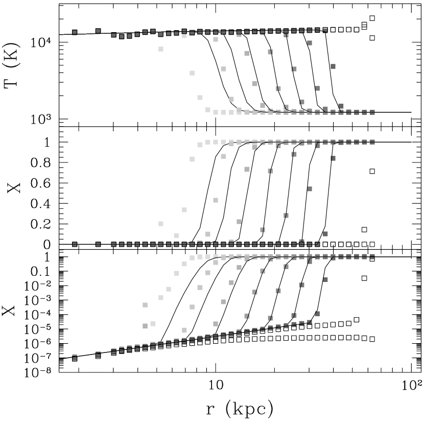
Figure 1: Propagation of the ionization front into the uniform neutral medium with $n=2.5\times 10^{-5}\mbox{\,cm}^{-3}$ from a point source with $\dot{N}_{\rm ph}=10^{52}\mbox{\,s}^{-1}$. Solid lines show the exact spherically symmetric solution, whereas grey symbols show the 3D approximate solution after 3, 6, 12, 25, 50, 100, and 200 hydrodynamic time steps (in the order of the increasing darkness of a symbol). Two sets of open symbols show the 3D solution after 700 and 1000 hydrodynamic time steps. The latter moment corresponds to the time when the entire computational box is optically thin. The upper panel shows the gas temperature, the middle panels shows the hydrogen ionization fraction on a linear scale, and the bottom panel shows the hydrogen ionization fraction on a logarithmic scale.

Figure 1 now illustrates how our scheme works for a case of a point source in a uniform medium. In this test the point source is located at the center of a $64^{3}$ mesh in a $70\mbox{\,kpc}$ box with periodic boundary conditions. The source spectrum contains only hydrogen ionizing photons. We notice that the approximate 3D solution converges to the exact solution in about 10 hydrodynamic time steps, after which time the 3D scheme reproduces accurately not only the position of the ionization front, but also its detailed temperature and ionized fraction profiles. The deviation at the initial moment is most likely due to finite resolution of the 3D code. At later times the ionization front leaves the computational box and the solution properly approaches the optically thin regime (open symbols in Fig. 1) when most of the box has a uniform radiation background and a proximity region exists around the source.

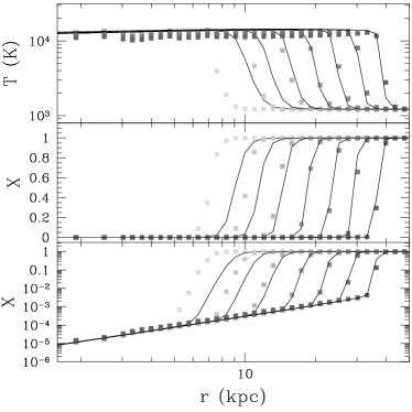
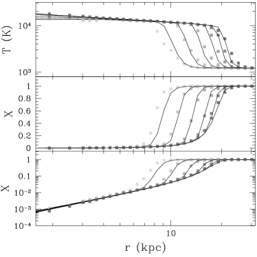
Figure 2: The same as Fig. 1 except for $\dot{N}_{\rm ph}=10^{50}\mbox{\,s}^{-1}$ (a) and $\dot{N}_{\rm ph}=10^{48}\mbox{\,s}^{-1}$ (b). In this case only first 200 hydrodynamic time steps are shown.

Figure 2 shows in two panels the same test with 100 and 10,000 weaker source respectively. Again, not only the position, but also the detailed profile of the ionization front is reproduced. In the latter case the source is so weak (by construction) that it reaches its Stromgen sphere before the ionization front leaves the box. We continued the weak source test for another factor of three in time and the solution remains undistinguishable from the last line shown with no trace of unphysical numerical diffusion propagating outside of the Stromgen sphere.

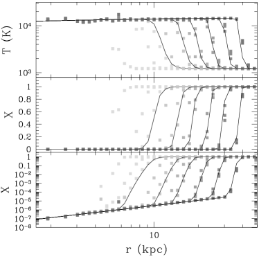
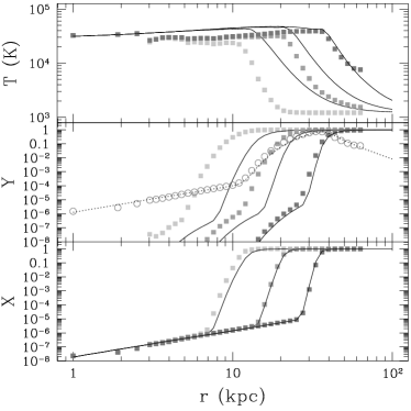
Figure 3: The same as Fig. 1 except (a) three sets of solutions shown corresponding to three choices for the hydrodynamic time step; (b) the source spectrum is a power-law with the slope of -1.25 and thus includes He i and He ii ionizing photons. In the latter case the middle panel shows the He i ionization fraction (filled symbols). Open symbols mark He ii ionization fraction at the last output. Only 6th, 25th, and 100th hydrodynamic time steps are shown.

Figure 3a shows the effect of changing the hydrodynamic time step. Three sets of filled symbols correspond to the hydrodynamic time step changed by a factor of $1/2$, 1, and 2 relative to Fig. 1. We again notice that about 10 hydrodynamic time steps after switching on of the source are sufficient to achieve complete convergence. Figure 3b also tests the performance of our scheme in the case when the ionizing spectrum extends to higher energies, thus being able to ionize He i and He ii as well as H i. In that case the agreement for helium is somewhat worse than for hydrogen, and it takes about 30 hydrodynamic time steps to converge on the helium profiles. This is however is still very small compared to the total number of hydrodynamic time steps in a realistic simulation, so that the compound error is expected to be negligible.

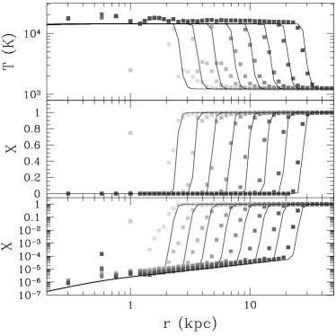
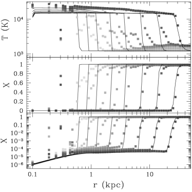
Figure 4: The same as Fig. 1 except that the density is not uniform by falls off as $r^{-1}$ (a) or $r^{-2}$ (b) with a small core at the center.

Figure 4 illustrates another two tests in which the density distribution is not uniform but falls off away from the source as the first or the second power of radius. In the latter case the profile of the ionization front at earlier times is not well reproduced due to the finite resolution of the 3D scheme.

4.2 Shadowing

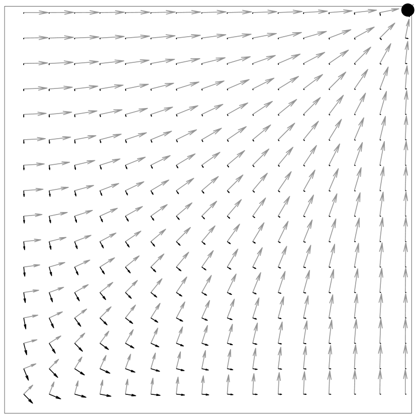
Figure 5: Two eigenvectors of the optically thin Eddington tensor in one quadrant of $z=0$ section of the computational box. The source location is labeled by a filled circle.

The tests from the previous section demonstrate that our scheme performs reasonably well for a single source in a spherically symmetric case. However, the choice of the optically thin Eddington tensor is, obviously, an approximation, and we can identify regimes where it is likely to fail. This is best illustrated by Figure 5, which shows the two eigenvectors of the optically thin Eddington tensor for a single source. The box has a unit side, and is located so that its center coincides with the point (0,0,0). The source is located at the center. We show the $x-y$ plane of the box with two eigenvectors laying in that plane. The eigenvectors are scaled by the square root of their respective eigenvalues (due to symmetry, the third eigenvector is directed along $z$ direction, but the respective eigenvalue is zero). Their signs therefore are undetermined, i.e. each vector can be turned around 180 degrees.

In this test case it is easy to find the exact Eddington tensor - it has only one nonvanishing eigenvalue (therefore equal unity everywhere because the trace of the Eddington tensor is identically equal unity) and the corresponding eigenvector at every point in space points towards (or away from) the source (i.e. $h^{ij}=e^{i}_{r}e^{j}_{r}$). The grey vectors in Fig. 5 show this eigenvector. However, in the optically thin case there exist another eigenvector, shown in black in Fig. 5. This eigenvector arises due to periodic boundary conditions as a contribution from periodic images of the source. As the result, the second eigenvector will allow for the propagation of the ionization front in the direction tangential to the source (albeit with a lower speed).

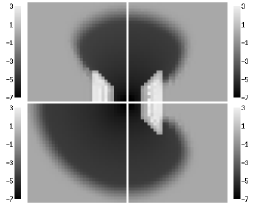
Figure 6: The distribution of neutral hydrogen in the one quadrant of the midplane of the computational box for four different tests: uniform medium (lower left panel), uniform medium with a 1000 times denser wedge (lower right panel), uniform medium with a wedge in a twice larger ($128^{3}$) box (upper right panel), uniform medium with a wedge with the exact Eddington tensor (upper left panel). All panels are flipped so that the source is located at the center of the plot. The side bars give the correspondence between the color and the decimal log of the neutral hydrogen density.

Figure 6 serves to illustrate this point. Its lower left panel shows the one quadrant in the midplane from a test shown in Fig. 1. Dark color shows the ionized region, and light color shows the still neutral medium. The lower right panel shows the same test (the panel is flipped around the $y$ axis) but with the 1000 times denser wedge inserted on the way of the ionization front. The wedge is supposed to shield the medium behind it from the ionizing radiation, however we can see the ionization front propagating behind the wedge with about 1/5 of the normal ionization front speed. This propagation is caused by the second eigenvector of the Eddington tensor, and is therefore unphysical - it is a manifestation of the optically thin Eddington tensor calculated in a periodic universe.

To verify that our conclusion is indeed correct, we have performed the same test in a twice larger box ($128^{3}$ instead of $64^{3}$) shown on the upper left panel of Fig. 6. In that case all the periodic images are twice further away, the contribution from them to the Eddington tensor is 4 times smaller, and we expect the tangential ionization front to propagate with $(1/4)^{1/3}=0.6$ times lower speed, as indeed can be observed from the figure.

Finally, we show the same test but calculated with the exact Eddington tensor on the upper left panel. In this case the ionization front does not propagate behind the wedge except by a very weak numerical diffusion (which is not important in a realistic simulation).

These tests illustrate the main shortcoming of the proposed scheme: the slow propagation of the ionization fronts behind the shadow. We emphasize that this propagation is quite slow, significantly slower than the ionization front speed. We notice this effect only because there should be no propagation of the radiation behind the shadow whatsoever. Our tests are not sufficient to evaluate whether this is a significant drawback or it is not important in realistic simulations - we expect that future work will shed light on this question.

In the proposed framework, we are not aware of the acceptable way to circumvent this deficiency of the scheme. We have tried to experiment with different choices of the Green functions for calculating the Eddington tensor, but found no noticeable improvement - with the following simple reason: if we adopt a Green function which falls faster than $1/r^{2}$ (a short-range one) in order to reduce the contributions from the distant periodic images, we at same time introduce deformations into the Eddington tensor inside the computational box, because of the periodicity of boundary conditions. These deformations may lead to even larger errors than the original optically thin Eddington tensor. Significant improvement over the proposed scheme is only possible if the Eddington tensor is estimated more accurately, for example, by calculating the exact tensor at a number of selected points inside the computational box. However, it seems unlikely this could be done with acceptable computational cost.

We again emphasize here that the fact that the Eddington tensor is calculated in the optically thin regime does not compromise shadowing by itself, but only due to imposed periodic boundary conditions. The reason that the shadowing works with the optically thin Eddington tensor is because the absorption of ionizing photons by the obstacle is computed essentially exactly (up to the RSL approximation, which becomes exact in the limit of a very dense obstacle). The optically thin approximation does make an error by assigning the incorrect values for the Eddington tensor behind the obstacle, but because the moments equations insure that the ionizing photon number density behind the obstacle is zero, the error in the Eddington tensor becomes irrelevant.

4.3 Multiple sources

It may appear that the choice of the optically thin Eddington tensor will also lead to a serious error in a case of several sources inside the computational box. Indeed, let’s consider two sources inside a computational box: a strong one and a weak one, and let’s assume that the two sources switch on simultaneously. Until their respective ionization fronts meet, each will have a spherical H ii region around it, and inside each of the H ii regions the Eddington tensor will be of the form $n^{i}n^{j}$ where $\vec{n}$ is the unit vector pointing toward the respective source. However, the proposed scheme adopts an optically thin Eddington tensor, which means that at each point in space the Eddington tensor is given by equation (22) with

$$P^{ij}={S_{1}r_{1}^{i}r_{1}^{j}\over r_{1}^{4}}+{S_{2}r_{2}^{i}r_{2}^{j}\over r_{2}^{4}},$$

where $\vec{r}_{1}$ and $\vec{r}_{2}$ are coordinates of the two sources in a reference frame tied to a given point in space, and $S_{1}$ and $S_{2}$ are their respective luminosities. We assume that $S_{1}>S_{2}$.

Near the strong source the contribution from the weak source is small, and thus the optically thin Eddington tensor is a good approximation to the exact one. However, near the weak (second) source the contribution from the first source could be important: even if $r_{2}<r_{1}$, $S_{1}>S_{2}$. However, the physics of the ionization fronts is such that this is not a significant problem. We can illustrate that with the following simple estimate.

The radius of the ionization front scales as a cubic root of the source luminosity. Thus, at the moment when the ionization fronts from the two sources overlap, the ratio of the front radii is

$$R1/R2=(S1/S2)^{1/3}.$$

The contribution to the tensors from each of the sources is proportional to $S/r^{2}$, i.e. the ratio of the contributions from the weak and the strong sources to the Eddington tensor within the weak source’s H ii region is

$${h^{ij}_{2}\over h^{ij}_{1}}={S_{2}r_{1}^{2}\over S_{1}r_{2}^{2}}.$$

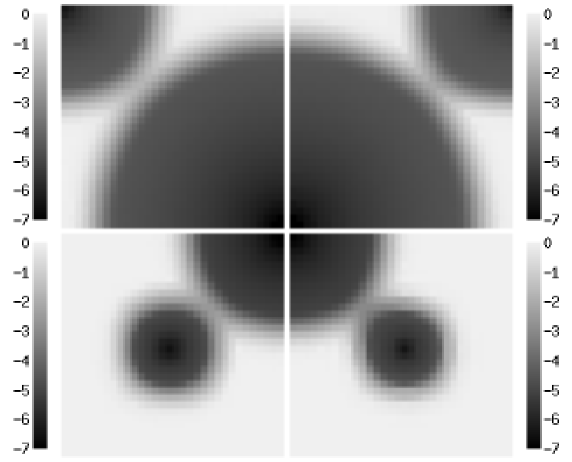
Figure 7: The distribution of neutral hydrogen in one quadrant of the midplane of the computational box for four different cases. The upper row shows the two source test with the weak source located at (-0.5,-0.5,0) and in the bottom row the weak sources is at (-0.25,-0.25,0). The strong source is at (0,0,0), and the ratio of source luminosities is 10. Left columns show the case with the exact Eddington tensors (which can only be calculated easily before the two ionization fronts overlap), and right columns show the test with optically thin Eddington tensors. In both cases the difference is noticeable but not large.

This contribution is greater than 1 (i.e. the weak source dominates its own Eddington tensor in the optically thin regime regime) when

$$\left(r_{2}\over R_{2}\right)^{2}<\left(r_{1}\over R_{1}\right)^{2}{R_{2}\over R_{1}}$$

or

$${r_{2}\over R_{2}}<{r_{1}\over R_{1}}\left(S_{2}\over S_{1}\right)^{1/6}.$$

Even at the time of overlap, when $r_{1}\sim R_{1}$, most of the volume inside the HII region around the weak source is dominated by the weak source, because $1/6$ is too weak a power law. Before the overlap, $r_{1}>R_{1}$ ($r_{1}$ is the distance from the strong source to a point inside the weak source H ii region), so the constraint is even weaker.

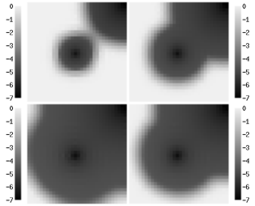
Figure 8: The distribution of neutral hydrogen in one quadrant of the midplane of the computational box for the two-source test with optically thin Eddington tensors at four different times.

Figure 7 illustrates this conclusion. The two two-source tests presented in the figure show that the effect of the stronger source on the propagation of the ionization front around a weaker source are small albeit still noticeable. We also show in Figure 8 consequent evolution for this test for the approximate solution. We are unable to compute the exact solution in this case because we cannot calculate the exact Eddington tensor when two H ii regions overlap.

4.4 Optically thin regime

Figure 9: The number of ionizing photons per baryon as a function of time for the optically thin case (dashed line) and for the full calculation (solid line) for the test presented in Fig. 1. The dotted line shows the optically thin case minus one (one photon per baryon is used to ionize the box).

One of the attractive features of this scheme is that the transition to the optically thin regime (or, more precisely, to the regime when the mean free path is much larger than the size of the computational box) is automatic, whereas in many alternative approaches it is not so trivial. Fig. 1 shows this regime for one of our tests with open symbols. In Figure 9 we show the ionizing background (i.e. the volume averaged specific intensity) measured in units of ionizing photons per baryon in the computational box for the optically thin case (no absorptions) and for one of our single source tests. The dotted line in this figure shows the optically thin case minus one, which approaches the full solution at later times. This illustrates the conservation of photons as the solution switches from the optically thick to the optically thin regime (in this test, recombinations are not important, and only one ionizing photon per baryon is needed to ionize the whole box).

This test illustrates that our scheme automatically insures the exact conservation of the number of photons as the mean free path crosses the box boundaries.

4.5 Realistic simulations

Figure 10: The evolution of the spatially averaged ionizing intensity $J_{\mbox{\small{\rm H\,\sc i}}}$ (measured in conventional units of $10^{-21}\mbox{\,erg}/\mbox{\,cm}^{2}/\mbox{\,sec}/\mbox{\,Hz}/\mbox{\,rad}$) in two simulations of a representative cosmological model: using the Local Optical Depth (LOD) approximation of Gnedin (2000, dotted line) and Optically Thin Variable Eddington Tensor (OTVET; solid line) approximation developed in this paper.

While the main purpose of this paper is to present the new and accurate approximation for modeling continuum radiative transfer, we give here also an example of how it performs for the problem it was developed for, cosmological reionization. For this purpose we have repeated one of the simulations from Gnedin (2000), namely the run labeled “N64_L2_A”. That simulation contained $64^{3}$ dark matter particles, an equal number of baryonic cells and, towards the end of the calculation, roughly the same number of stellar particles in a computational box with the size of $2h^{-1}$ comoving Mpc. A reader can find a full description of this simulation in Gnedin (2000) and we do not repeat it here for brevity. This test allows us not only to check the performance of our Optically Think Variable Eddington Tensor (OTVET) approximation in a realistic cosmological simulation, but also to compare it with the much less accurate Local Optical Depth (LOD) approximation. The OTVET radiative transfer simulation presented here consumed roughly three times the computational time than the one using LOD transfer.

In Figure 10 we show the evolution of the volume averaged ionizing intensity for two simulations. The two simulations have identical parameters and the same physical content - the only difference is in the method used to solve for the radiative transfer. We notice here that the two simulations are qualitatively similar, and reionization (the sharp rise in the specific intensity at around $z=7$) occurs almost at the same time in both simulations. This should be expected because the LOD approximation is designed to give the correct time for the overlap of H ii regions, which marks the time of reionization. However, there are also noticeable differences, which we attribute to the inaccuracy of the LOD approximation.

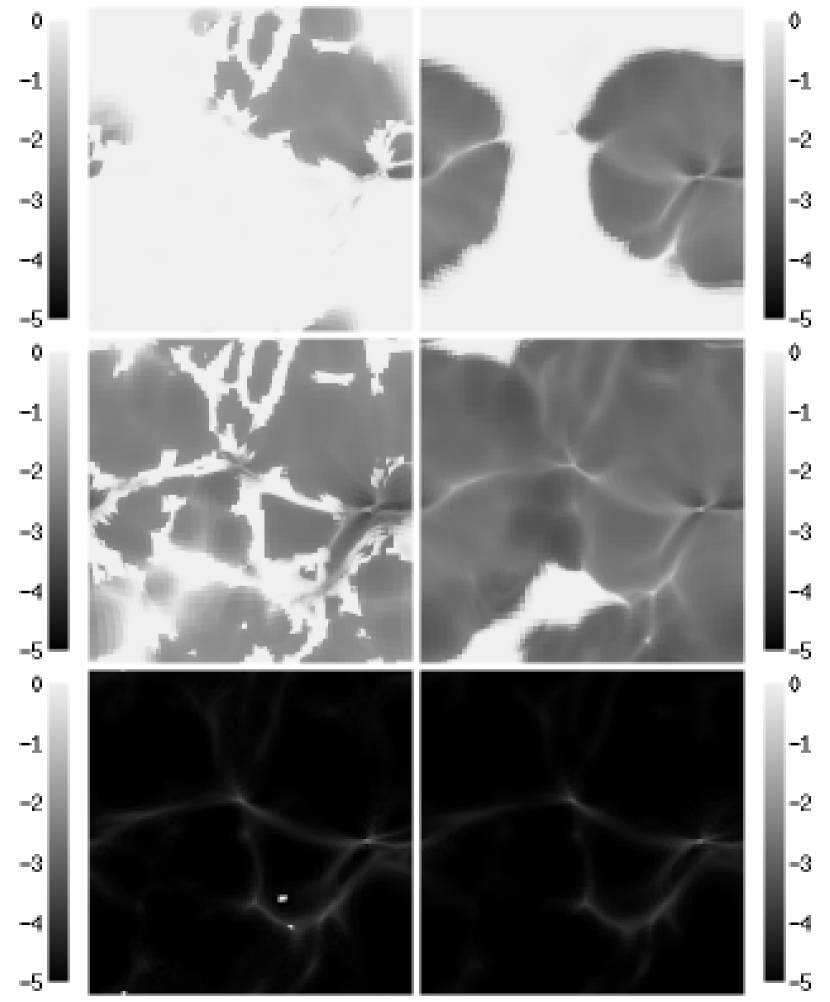
Figure 11: The distribution of neutral hydrogen in a realistic simulation of cosmological reionization at three different times as shown in three rows: before the overlap of H ii regions (top row), during the overlap (middle row), and after the overlap (bottom row). The left column shows the highly approximate solution with the Local Optical Depth (LOD) approximation from Gnedin (2000), and the right column shows the present scheme (OTVET).

In order to investigate these differences further, we show in Figure 11 slices from two simulations at three different times - before the overlap of H ii regions, during the overlap, and after the overlap. We notice that while large-scale features are similar in two simulations, small-scale structure is quite different. The main difference is the excess of low density neutral gas in the LOD approximation. This is indeed expected, because the LOD approximation makes the largest error in the regions with the optical depth is about unity.

It appears from Fig. 11 that this error is systematic - neutral regions are always larger in the LOD approximation - and thus the LOD approximation performs worse than one of the authors (NG) hoped for. On the other hand, the LOD approximation only reproduces the ionization fronts speed on average, i.e. it does not guarantee a correct speed for every ionization front. The fact that the large-scale structure of ionization fronts agrees quite well between the two simulations indicate that the ionization front speed in the LOD approximation is calculated more accurately than could be expected a priori. This observation would allow to improve the LOD approximation by correcting the systematic deviation on the $\tau\sim 1$ regime.

Another significant difference between the two approximations is a higher asymmetry of H ii regions at early times in the LOD approximation. This difference arises because the LOD approximation estimates the total optical depth to the source from its local density. Somewhat denser material becomes therefore artificially more difficult to ionize. Consequently, I–fronts wrap around dense material unphysically strongly giving rise to the strongly distorted ionization fronts observed in Figure 11.

Finally, at later times (after the overlap) the two solutions are quite similar (except for small errors in the LOD approximation in the $\tau\sim 1$ regime) because both approximations become exact in the optically thin regime.

5 Conclusions

We present a new approach to numerically model continuum radiative transfer based on the Optically Thin Variable Eddington Tensor (OTVET) approximation. Our method insures the exact conservation of the photon number and flux (in the explicit formulation) and automatically switches from the optically thick to the optically thin regime. It scales as $N\log N$ with the number of hydrodynamic resolution elements and is independent of the number of sources of ionizing radiation (i.e. works equally fast for an arbitrary source function).

We also describe an implementation of the algorithm for the Soften Lagrangian Hydrodynamic code (SLH). We present extensive tests of our method for single and multiple sources in homogeneous and inhomogeneous density distributions, as well as a realistic simulation of cosmological reionization.

The method fully solves the cosmological radiative transfer equation in a conservative fashion via moment equations. The only approximation is our use of optically thin Eddington tensors. One may envision to employ a Monte Carlo or short characteristic methods to supply more accurate tensors for applications in which an even more accurate knowledge of the isotropy of radiation field is required.

The main shortcoming introduced by optically thin Eddington tensors with periodic boundary conditions is the unphysical propagation of ionization fronts behind an optically thick obstacle. This diffusive effect is however slow and negligible for the typical R–type ionization fronts of interest in numerical cosmology.

A realistic simulation of cosmological reionization with our current implementation of the new method took approximately three times the computing time than a simulation without radiative transfer. However, there are several optimizations which we have not yet implemented, which will shorten this time by at least a factor of two.

T.A. acknowledges stimulating and insightful discussions with Markus Ramp, Dimitri Mihalas, Pascal Paschos and Michael Norman. We are also grateful to the referee Andreas Burkert for friendly and valuable comments. This work has partially been supported through NSF grants ACI96-19019 and AST-9803137, as a part of GC³, and by National Computational Science Alliance under grant AST-960015N, and utilized the SGI/CRAY Origin 2000 array at the National Center for Supercomputing Applications (NCSA).

References

- Abel & Mo (1998) Abel, T., & Mo, H. J. 1998, ApJ, 494, L151
- Abel et al. (1999) Abel, T., Norman, M. L., & Madau, P. 1999, ApJ, 523, 66
- Barkana & Loeb (2001) Barkana, R., & Loeb, A. 2001, Phys. Rep., in press
- Ciardi et al. (2001) Ciardi, B., Ferrara, A., Marri, S., Raimondo, G. 2001, MNRAS, in press (astro-ph/0005181)
- Gnedin (1995) Gnedin, N. Y. 1995, ApJS, 97, 231
- Gnedin (2000) Gnedin, N. Y. 2000, ApJ, 535, 530
- Gnedin & Bertschinger (1996) Gnedin, N. Y., & Bertschinger, E. 1996, ApJ, 470, 115
- Gnedin & Ostriker (1997) Gnedin, N. Y., & Ostriker, J. P. 1997, ApJ, 486, 581
- Haehnelt (1995) Haehnelt, M. G. 1995, MNRAS, 273, 249
- Haiman et al. (2000) Haiman, Z., Abel, T., & Rees, M. J. 2000, ApJ, 534, 11
- Kepner et al. (1999) Kepner, J., Tripp, T. M., Abel, T., & Spergel, D. N. 1999, AJ, 117, 2063
- Kessel-Deynet & Burkert (2000) Kessel-Deynet, O., & Burkert, A. 2000, MNRAS, 315, 713
- Norman et al. (1998) Norman, M. L., Paschos, P., & Abel, T. 1998, MmSAI, 69, 455
- Razoumov & Scott (1999) Razoumov, A. O., & Scott, D. 1999, MNRAS, 309, 287
- Silk & Rees (1998) Silk, J., & Rees, M. J. 1998, A&A, 331, L1
- Sokasian et al. (2001) Sokasian, A., Abel, T., & Hernquist, L. 2001, NewA, submitted