Modified Dust and the Small Scale Crisis in CDM
Fabio Capelaa and Sabir Ramazanovb
a DAMPT, Centre for Mathematical Sciences, Cambridge University,
Wilberforce Road, Cambridge CB3 0WA, UK
b Service de Physique Théorique, Université Libre de Bruxelles (ULB),
CP225 Boulevard du Triomphe, B-1050 Bruxelles, Belgium
Abstract
At large scales and for sufficiently early times, dark matter is described
as a pressureless perfect fluid—dust—non-interacting with Standard Model fields.
These features are captured by a simple model with two scalars: a Lagrange multiplier and
another playing the role of the velocity potential.
That model arises naturally in some gravitational frameworks, e.g., the mimetic
dark matter scenario. We consider an extension
of the model by means of higher derivative terms,
such that the dust solutions are preserved
at the background level, but there is a non-zero sound speed at the linear level.
We associate this Modified Dust with
dark matter, and study the linear evolution of cosmological perturbations in that picture.
The most prominent effect is the suppression of their power
spectrum for sufficiently large cosmological momenta. This
can be relevant in view of the problems that cold dark matter faces at sub-galactic scales,
e.g., the missing satellites problem. At even shorter scales,
however, perturbations of Modified Dust are enhanced compared to the predictions
of more common particle dark matter scenarios. This is a peculiarity of their evolution
in radiation dominated background. We also briefly discuss clustering
of Modified Dust. We write the system of equations in the Newtonian
limit, and sketch the possible mechanism which could prevent
the appearance of caustic singularities. The same mechanism may be
relevant in light of the core-cusp problem.
1 Introduction
To date, particle physics provides us with a plethora of candidates for dark matter (DM). These include sterile neutrinos, supersymmetric partners of the Standard Model particles, light scalars (axions) and many others. Given that the new degrees of freedom are heavy enough and weakly interacting with the Standard Model constituents, one deals with cold dark matter (CDM). The concept of CDM is of the uttermost importance in modern cosmology. Namely, it is among the building blocks of the 6-parametric concordance model established by the recent Planck and WMAP missions [1, 2]. In particular, the evolution of linear perturbations developed in this framework is in excellent agreement with the picture of the Cosmic Microwave Background temperature anisotropies [3]. Furthermore, simulations based on CDM lead to correct predictions about the large scale structure distribution in the Universe [4, 5, 6]. Finally, the concept of CDM agrees with the Bullet Cluster observations [7, 8] and provides an explanation for the flat galaxy rotation curves [9, 10, 11].
Despite these successes, there is some tension between CDM predictions and astronomical data at the sub-galactic scales. This amounts to three problems. First, CDM predicts an overabundance of small structures, i.e., dwarf galaxies. Observations in the vicinity of the Milky Way, however, indicate a much smaller number. This states the “missing satellites problem” [12, 13]. Second, CDM leads to cuspy profiles of the DM halos [9, 10]. At the same time, observations on the concentrations of dwarf galaxies rather prefer cored profiles [14, 15]. Finally, N-body simulations result into a large central density of massive subhaloes in the Milky Way—a fact, which is in conflict with observations of stellar dynamics in dwarf galaxies hosted by those subhaloes. This inconsistency is dubbed as the “too big to fail” problem [16]. It is important to keep in mind that the aforementioned shortcomings of CDM may not be robust to the proper account of various astrophysical phenomena [17, 18, 19, 20, 21, 22, 23, 24, 25]. However, realistic high resolution numeric simulations, which include baryonic processes, are challenging to implement at the moment. Meanwhile, it is interesting to speculate if part or all of the problems are due to the peculiar nature of DM itself. For example, Warm Dark Matter (WDM) scenarios start from the proposal that the DM particles are still mildly relativistic at the freeze out temperature. Then, the short wavelength perturbations get washed out due to free streaming processes [26, 27]. This provides a simple mechanism to suppress the number of small scale structures, and thus can be relevant to alleviate the missing satellites problem [28]. However, WDM scenarios are perhaps too efficient in erasing the short wavelength perturbations, as indicated by the constraints following from the Lyman- forest data [29]. Another approach to the problems at the sub-galactic scales is to go beyond the approximation of collisionless matter. Namely, allowing for sufficiently strong self-interactions of DM particles [30], one can address the core-cusp and too big to fail problems [31]. On the other hand, constraints obtained from the Bullet Cluster observations imply smaller self-interaction cross-sections than what is required in view of the core-cusp problem [32].
One can try to find a solution to the small scale crisis by switching to a paradigm different from particle DM. Recently, an interesting proposal on the way to model dark matter and dark energy has been made in Ref. [33]. There, the authors introduced a novel class of theories, referred to as the -fluid. The action for the -fluid is given by
| (1.1) |
In what follows, we assume the sign convention for the metric. Here is the Lagrange multiplier; is some arbitrary function of the scalar and its derivatives. Varying the action (1.1) with respect to the field enforces the constraint , so that is a unit 4-vector. One can associate the field with the velocity potential of the -fluid. The constraint equation tells us that the fluid elements follow geodesics, much in the same manner as the dust particles. At the same time, given the non-trivial function , one can allow for a non-zero effective pressure with a time-dependent equation of state. This opens up the possibility to construct a fluid, which may mimic dust at early times and a positive cosmological constant later on.
In the present paper, however, we restrict the discussion to DM. A pressureless perfect fluid is obtained for the function identically equal to zero, i.e., . The energy density of the dust is associated with the field decaying as with the scale factor . It is thus tempting to view the construction with the Lagrange multiplier as the simplest model of DM: at the background and linear levels, it reproduces all the successes of more common particle scenarios. In the non-linear regime, however, the dust model has important drawbacks: it leads to caustic singularities and is unable to form stable DM halos [34].
From now on, we should go beyond the approximation of a pressureless perfect fluid. In the theory described by the action (1.1), this is achieved by incorporating the function . At the same time, we would like to keep the simple form of the background dust solutions in the Universe dominated by the -fluid: . Interestingly, this is possible with the non-trivial choice of the function ,
| (1.2) |
Here and are parameters with dimension of mass squared. Expressions (1.1) and (1.2) state the model, which we refer to as Modified Dust in what follows. We shortly give a brief summary of our main results. Before that, let us comment on how the action (1.1) arises in different gravitational frameworks.
In Ref. [35], the authors considered the standard Einstein’s metric as the composition of an auxilliary metric and the first derivatives of the scalar field ,
Unexpectedly, variation with respect to the fields and results in a modification of the Einstein–Hilbert equations such that the traceless part is non-zero even in the absence of matter. This discrepancy with the standard equations of General Relativity is due to the presence of an extra degree of freedom, which behaves as dust. The dust solution has been dubbed as mimetic dark matter in Ref. [35]. Soon afterwards, it has been realized that the proposed scenario is equivalent to adding a Lagrange multiplier into the Einstein–Hilbert action [36]. This is the picture described by the action (1.1). Furthermore, in Ref. [37] it was proved that the condition set on the initial Cauchy surface is sufficient to avoid ghosts. The concept of mimetic dark matter could be interesting from at least two perspectives. First, it is in direct relation with the broken disformal transformations in gravity [38]. Quite surprisingly, mimetic dark matter also arises in the context of non-commutative geometry, which might be a promising setup for quantum gravity [39]. Strictly speaking, the function equals to zero in the mimetic dark matter scenario as it stands. Setting it by hands, however, opens up the possibility to mimic different types of cosmologies [40, 41].
Constructions introducing the term with the Lagrange multiplier are known in the context of Einstein–Æther (EA) models [42]. In particular, scalar EA [43] has exactly the form given by Eqs. (1.1) and (1.2). This is interesting, as the scalar EA appears in the IR limit of the projectable version of Horava–Lifshitz model [44, 45, 46]— power counting renormalizable theory of gravity [47]. It is thus not a surprise that DM has been identified in this setup [48]. Contrary to the case of Modified Dust, however, it was suggested in [48, 49] to extend the pressureless perfect fluid by means of higher curvature terms inherent to Horava’s proposal.
In the present paper we prefer to stay on a more phenomelogical side. Our main purpose is to study the linear evolution of cosmological perturbations of Modified Dust described by Eqs. (1.1) and (1.2). We uncover several effects, which can be relevant in light of the small scale crisis. The first is the suppression of perturbations with relatively large momenta. As we will see explicitly in Section 2, -terms result into a non-zero sound speed at the level of perturbations [40]. Beyond the sound horizon, perturbations of Modified Dust behave as in the CDM picture: they grow linearly with the scale factor during the matter dominated (MD) stage. As they enter the sound horizon, their growth stabilizes. This places an important cutoff on the linear power spectrum in our model. In this regard, Modified Dust carries similarities with WDM. So, by setting , where is the Planck mass111Hereafter, we define the Planck mass squared as the inverse of the Newton’s constant , i.e., ., one can suppress perturbations with wavelengths below . Hence, Modified Dust is capable to address the missing satellites problem. There is, however, an important distinction from the case of WDM scenarios. The difference is clearly seen from the evolution during the radiation dominated (RD) stage, when perturbations of Modified Dust of very small wavelengths experience a linear growth with the scale factor. We show this explicitly in Section 3. As a result, corresponding perturbations get amplified compared to the predictions of WDM scenarios (and even CDM scenarios for sufficiently large redshifts). The effect, however, is only prominent for wavelengths in the pc-range. Therefore, its possible physical applications remain unclear at the moment.
Finally, in Section 4 we discuss the behaviour of Modified Dust in the non-linear regime. This is particularly relevant in light of caustic singularities occuring in the case of pressureless perfect fluid. We notice, however, that deviations of Modified Dust from its conventional counterpart become prominent exactly where one expects the appearence of singularities. Based on this simple observation, we propose a mechanism that could be relevant to reduce the energy density in the dangerous regions.
The outline of the paper is as follows. In Section 2, we discuss the evolution of the Universe filled in with Modified Dust. This we do at the background level and at the level of linear perturbations. In Section 3, we discuss peculiarities of the linear evolution at very early times, during the RD stage. In Section 4, we get back to the MD Universe and write down the relevant system of cosmological equations in the Newtonian limit. There, we discuss the clustering issues of Modified Dust. We finish by formulating some opened issues in the last Section.
2 Matter Dominated Universe
We start with the case of the Universe dominated by Modified Dust. This is a good approximation to the Universe at relatively low redshifts, i.e., , when the contribution of the radiation can be neglected. Non-trivial effects arising upon the inclusion of radiation will be considered in the next Section. In the present paper, we will always neglect the contributions from baryons and dark energy. The former is expected to change the behaviour of the gravitational potential at the percent level, while the latter becomes relevant only at very small redshifts, .
2.1 Case
In the simplest case, when the constants equal to zero, i.e., , we have for the energy momentum tensor of the -fluid,
Varying the action (1.1) with respect to the field (Lagrange multiplier), one obtains
| (2.1) |
We see explicitly that the energy momentum tensor is the one of a pressureless perfect fluid, with being the energy-density and the velocity potential. At the background level, the former drops with the scale factor as . We fix the constant in a way that corresponds to the energy density of DM, i.e.,
| (2.2) |
The background value of the field is given by
up to an irrelevant constant of integration. The cosmological evolution of the Universe filled in with dust is then obtained from the -component of Einstein’s equations,
| (2.3) |
Here , where denotes the Hubble parameter. From this point on we prefer to work in terms of the conformal time . The prime denotes the derivative with respect to the latter. From Eq. (2.3) we obtain , which gives the standard solution for the scale factor in the matter dominated Universe: .
Note one generic feature of the model, where the 4-velocity of the fluid is the derivative of the scalar field , i.e., . In that case, the conservation of the energy-momentum tensor implies just one equation. Indeed,
where we took into account Eq. (2.1). Consistently, this equation can be obtained from the variation of the action (1.1) with respect to the field . Of course, this does not lead to degeneracy of solutions, as the constraint (2.1) itself plays the role of the missing equation [40].
At the linear level, Eq. (2.1) reads
| (2.4) |
This is essentially the Euler equation linearized, where is the scalar perturbation of the -component of the metric. Hereafter, we choose to work in the Newtonian gauge. As it follows from the form of the action (1.1), Eq. (2.4) remains unmodified even for the non-trivial choice of the function . In particular, the same equation is true for the case of non-zero coefficients and , to which we will turn soon.
Before that, let us remind the picture of linear evolution in the case of the pure dust (CDM). In the Newtonian gauge, the perturbed Friedmann–Robertson–Walker metric has the form,
In the perfect fluid approximation, the simple relation holds between the potentials and : . We choose to work with the function in what follows. The evolution of the potential can be easily inferred from the -component of Einstein’s equations,
Up to a negligible decaying mode, it has the constant solution . In the presence of the constant gravitational potential, perturbations of DM grow linearly with the scale factor, as it immediately follows from the Poisson equation,
| (2.5) |
where is the Newton’s constant. That is, during the MD stage, perturbations of DM are subject to the Jeans instability independently of their momenta. Later on, they enter non-linear regime, and the clustering starts. This standard picture changes drastically upon the inclusion of -terms.
2.2 Generic case
Let us make two important comments before we dig into the details of calculations. With no loss of generality, we choose to work with the unique coefficient in the bulk of the paper, while setting the other one, , to zero. Besides considerations of simplicity, this is also justified, since both terms are expected to result into qualitatively the same phenomenology. We put the details regarding the case in the Appendix B. With this said, the energy momentum tensor has the form [40],
| (2.6) |
where .
For non-zero coefficients and the interpretation of the field as the energy-density of DM may be misleading. Still, we prefer to stick to the simple convention (2.2) in what follows. Hopefully, this is not going to confuse the reader, as one is interested in the behaviour of the gravitational potential in the end. Moreover, the difference between the formal energy density and the physical one, , remains small in most cases discussed in the present paper. This is true at both levels of background and linear perturbations. The only exceptional case occurs at very early times, deeply in radiation dominated era. We will comment on that in due time.
Let us write the background cosmological equations. The simplest is the one corresponding to the -component of Einstein equations,
| (2.7) |
Apart from the degenerate case , we have , which corresponds to the Universe driven by dust. Consistently, the conservation equation has the form,
| (2.8) |
The Friedmann equation is given by
Upon the formal change , we get back to the standard set of equations of the dust dominated Universe. In Appendix B, we show that the same conclusion holds for the -term in Eq. (1.2).
Before turning to the study of linear perturbations, let us make one useful observation. We note that the linearized energy-momentum tensor is similar to that of a perfect fluid in a sense that . This means that one can impose the constraint on the scalar perturbation of the spatial part of the metric, 222The analogous conclusion is not applicable to the -term. However, the difference between potentials and is negligible and hence is irrelevant for phenomenology. See details in Appendix B. We thank A. Vikman for discussions on this point.. We choose to work with the potential in what follows.
The simplest way to proceed is to write the -component of Einstein’s equations. The reader can find the explicit expression in the Appendix A. Here we write it in the approximation of the small parameter , i.e., ,
| (2.9) |
where is given by
Clearly, the second term in the equation mimics the sound speed 333This observation was first made in the context of inflation [40].. This explains the notation “” we use. Provided that the cosmological modes are beyond the speed horizon, i.e., , one obtains for the field perturbation . Using Eq. (2.4), we get . This is the standard solution for the gravitational potential in the MD Universe. Another story occurs after the modes enter the sound horizon, i.e., in the regime . Accordingly to Eq. (2.9), the rapid growth of the perturbations of the field stops and turns into oscillations, i.e., . As a result, the gravitational potential decreases with the scale factor.
The behaviour of the DM energy density perturbations can be easily deduced from the -component of Einstein’s equations, which takes the standard form (2.5) in the small approximation. As it follows, for modes with sufficiently short wavelengths and at relatively late times, the linear growth of the energy density contrast stabilizes and turns into oscillations with a constant amplitude. Let us choose the constant in such a way that the growth stops at redshifts as small as for perturbations with the comoving wavelengths of . These wavelengths roughly characterize the collection regions collapsing to the halos of dwarf galaxies. The redshifts correspond to the times, when the modes of interest enter the non-linear regime (in the CDM picture). The estimate of the parameter reads , which is remarkably close to the Grand Unification Scale. This value of the parameter is required to alleviate the missing satellites problem. For larger values, one risks to affect the evolution of the galaxies in an unaffordable manner. Much smaller values are, however, plausible, as the proper account of baryonic processes may eliminate the problem with the dwarf galaxies. In that case, however, the motivation for Modified Dust is essentially lost. Therefore, we set in what follows, unless the opposite is stated.
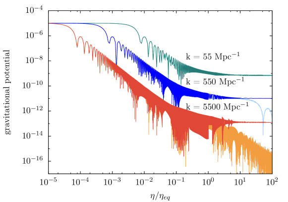
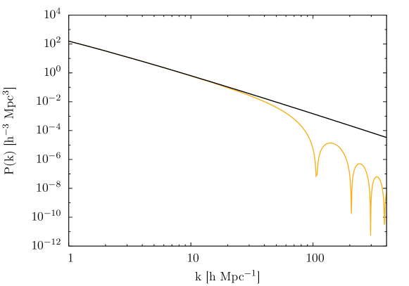
To put things on solid ground, we performed numerical simulations to obtain the gravitational potential and the matter power spectrum. The results are presented in Figs. 1 and 2, respectively. As it is clearly seen from Fig. 1, the gravitational potential deviates from the standard behaviour predicted by the CDM scenarios for sufficiently large cosmological momenta. Namely, at some point in MD stage it starts to oscillate with a decreasing amplitude and a frequency . The corresponding period of oscillations is very large: for wavelengths it is comparable with the age of the Universe. The decrease of the gravitational potential with the scale factor translates into the suppression of the linear matter power spectrum, which we plot in Fig. 2 for the redshift value . The choice of the redshift is dictated by simplicity considerations: for smaller values of , we would need to incorporate the effects of the accelerated expansion of the Universe into the analysis. Note that the plot in Fig. 2 represents the extrapolation of the linear evolution of Modified Dust to late times. This is by no means justified, as the cosmological modes of interest are deeply in the non-linear regime at the redshift . Still, the plot is useful for the purpose of comparison with the particle DM scenarios. We use the conventional definition of the power spectrum,
Here is the amplitude of the matter perturbations related to the two-point correlator in the coordinate space by
The picture 2 is quite analogous to what one has in the case of WDM scenarios [50, 51]. There are two important qualifications, however. While WDM models predict the exponential suppression of the small scale spectrum, we observe a more moderate power law drop. This distinction might be relevant, since WDM does perhaps too good job with diluting sub-galactic structures. Second, we note the presence of slow oscillations in the high momentum tail of the Modified Dust spectrum. This could be a promising smoking gun of our scenario.
The conclusions of the present Section work well for wavelengths in the kpc-range. For perturbations with even smaller wavelengths another effect becomes prominent. That is, very small perturbations get enhanced during the evolution in the RD epoch (once again, compared to the predictions of CDM). We discuss this issue in the following Section.
3 Inclusion of radiation
3.1 Initial conditions
In the presence of radiation, the evolution of Modified Dust changes considerably. In particular, the energy density associated with the field is now given by
| (3.1) |
Here is the energy-density corresponding to pure dust, i.e., . The novel contribution mimics radiation. The solution (3.1) follows from Eq. (2.8), where we set . The latter is the standard expression for the Hubble parameter during the RD stage. The term is somewhat worrisome, as it has a negative sign. It governs the evolution of the DM at redshifts as large as444At these early times the notion of“Modified Dust” appears to be misleading, as the -fluid also mimics radiation in that case. However, we choose to continue with our standard convention in what follows. . The value corresponds to the point, when . The temperature of the Universe at these early times reads . As these temperatures have taken place in the hot Big Bang cosmology, we conclude that deep in the RD epoch. This, however, does not imply the violation of the weak energy condition. As pointed out in the previous Section, is not the physical energy-density. The latter is given by and remains positive. Moreover, due to the time-dependence of the term , it can be absorbed into the standard radiation with no physical consequences at the background level.
Let us discuss the linear perturbations around the background (3.1). At very early times corresponding to the redshift values all the relevant modes are beyond the horizon. In the super-horizon regime, i.e., when , the conservation equation for the DM (A.9) takes the form,
The solution to this equation reads simply
| (3.2) |
where is the constant in time, which will be specified below. At very early times, formally as , the second term on the r.h.s. is the most relevant. In the same limit . Consequently, we obtain for the energy-density contrast at very early times ,—the standard adiabatic initial condition for radiation. As a cross check of our calculations, we observe that this initial condition is consistent with the limit of the -component of Einstein’s equations, see Eq. (A.6) of Appendix A.
To conclude, at very early times Modified Dust cannot be distinguished from radiation. This is true at both levels of the background and linear perturbations. The things are different for sufficiently late times, i.e., at the redshifts . In that case, Modified Dust takes the standard form, i.e., . The first term on the r.h.s. of Eq. (3.2) corresponds to the constant mode of the energy-density contrast , while the second term stands for the decaying mode. Neglecting the latter, we get the initial condition for Modified Dust, , where is the present energy density of DM. We fix the constant in such a way that we do not encounter problems with CMB observations. That is, we impose initially.
A comment is in order before we proceed. Working in terms of the quantity can be misleading at the redshift , when . At that point, we have . This, we believe, is just a formality, since the quantity —more relevant one–remains finite at all times. To avoid the problem, we could always provide the calculations in terms of and then convert the latter into .
3.2 Sub-horizon evolution
During the RD stage, cosmological perturbations follow a non-trivial evolution, which is particularly prominent for short wavelength modes. At sufficiently early times, the main contribution to the gravitational potential follows from the perturbations of radiation. In that case, the potential is given by [52]
| (3.3) |
where is the sound speed of radiation. The evolution of the energy-density perturbations can then be obtained in a straightforward manner by integrating the equation (A.9). We write down the solution,
| (3.4) |
The first two terms on the r.h.s. represent the well-known constant and logarithmically growing mode in CDM, while the third one is the novelty. It describes a mode linearly growing with the scale factor. This originates from the term in the conservation equation (A.9).
While for long wavelength modes this term is negligble, it may start to dominate for shorter ones at some point. This point in the linear evolution is defined from
| (3.5) |
Note that the effect takes place only for momenta larger than
| (3.6) |
otherwise, the condition (3.5) formally takes place at the MD stage , i.e., at , when the formula (3.3) and, consequently, the estimate (3.6) are not applicable. Here and denote the redshift value and the conformal time at the equilibrium between radiation and matter, respectively, and . For the value , we have , which corresponds to wavelengths . Perturbations with these wavelengths are expected to be amplified by the end of the RD stage.
The linear growth continues until the point in the evolution, when the DM perturbations become the dominant source of the gravitational potential. The associated redshift value is defined from
| (3.7) |
In this estimate, we took into account that perturbations of radiation do not grow, but experience oscillations with the amplitude [53]. Since this point on, the formula (3.3) is not applicable anymore. To handle the situation, let us get back to the conservation equation (A.9), where we omit all the terms except for one proportional to . Expressing the energy density contrast through the perturbations of the velocity potential , substituting into Eq. (A.6) and omitting the subleading terms, we obtain the second order equation for the density perturbations,
This equation has only oscillatory solutions. That is, the growth of perturbations stops and we get back to the picture observed in the matter dominated Universe. To quantify the amplitude of the oscillations, we first estimate the redshift value . By comparing Eq. (3.4) with the estimate (3.7), we obtain
Substituting this back into Eq. (3.7), we have for the amplitude of the energy-density perturbations,
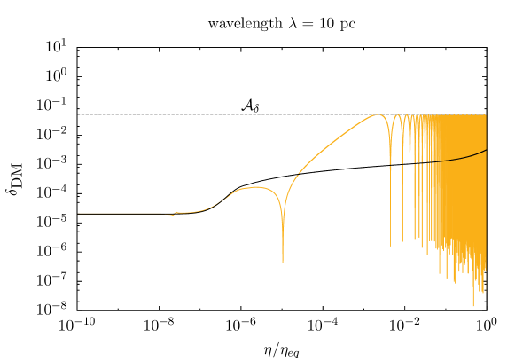
In Fig. 3, we plot the result of numerical simulations for the evolution of the energy density contrast . As it is clearly seen, it agrees well with our estimates. The associated gravitational potential also gets enhanced compared to the predictions of CDM scenarios, as it is sourced by perturbations of Modified Dust already at redshifts . This enhancement gets compensated for the wavelengths , since the gravitational potential remains constant in the CDM picture at the MD epoch, while it drops with the scale factor in the Modified Dust scenario.
Interestingly, for very short wavelengths, , the energy density contrast reaches unity already during the RD stage. We are led to the picture where the Universe becomes inhomogeneous at tiny scales already at large redshifts. This picture is in contrast to more common WDM and even CDM scenarios, where very small scale perturbations are washed out by free-streaming processes. In the future, it would be interesting to see, if that phenomenon implies any relevant consequences for observations. Though the pc-range of wavelengths is far out of reach for cosmological experiments, it may have important applications for the formation of primordial black holes, gravitational lensing, etc. This discussion is out of the scope of the present paper.
Before we finish the discussion about the evolution in the RD background, let us make a comment. We remind that generically perturbations are washed out below the free-streaming wavelengths of the photon. Naively, this effect can be a threat to the mechanism we discussed in this Section. Let us show that this never happens in fact. Indeed, the comoving free-streaming wavelength drops as with the redshift . We are interested in the value of at the times, when DM starts to dominate the linear evolution. This can be inferred from the value of at the recombination epoch,
Here is the redshift corresponding to the recombination epoch. As it is clearly seen, for the perturbations with the wavelengths , . Hence, one can neglect the free-streaming effects for all interesting wavelengths.
4 Non-linear level
Finally, let us discuss the behaviour of Modified Dust in the non-linear regime, i.e., when . Generically, non-linear analysis is a very complicated task, involving non-trivial numerical simulations. We leave this for the future work. What one can actually do at the moment is to write the relevant system of equations in the Newtonian limit, and discuss their possible physical consequences.
Before that, let us remind the state of affairs with the collisionless particle DM. In that case, one normally runs the N-body simulations, which attempt to solve the system of Vlasov–Poisson equations. The problem can be paraphrased in terms of the momenta of the Vlasov equation (collisionless Boltzmann equation). Formally, it leads to an infinite chain of coupled equations. Setting to zero all the momenta of the probability density starting from the velocity dispersion, results into the set of equations of the standard dust. That is, the conservation equation,
and the Euler equation
| (4.1) |
In the present Section, we omit the subscript “DM” in the notation of the energy density of Modified Dust. This system coadded with the Poisson equation can be solved iteratively using Eulerian or Lagrangian perturbation schemes [54, 55]. In the mildly non-linear regime the results are argued to be in a good agreement with N-body simulations. Furthermore, peaks of the energy density localized at the surface of particle crossing (caustics, or Zel’dovich pancake) give a qualitatively correct picture of the Cosmic Web. Since this point on, however, the dust approximation breaks down. That is, the divergence of the velocity and the energy density become infinite at the caustics, i.e., and 555Strictly speaking, this type of divergence is seen in the Zel’dovich approximation. It is argued, however, that the latter becomes exact for particular initial conditions. Moreover, corrections to the Zel’dovich approximation do not cure the problem.. The singularity has a clear physical meaning: it reflects the fact that the dust particles may pass unaffected through each other. After particles cross, they fly away from the caustics, as there is no mechanism sticking them together. This leads to fast broadening of the Zel’dovich pancake, and eventually to diluting the structures [34]. The problem does not occur in the case of the real particle DM: near the caustics high momenta of the Vlasov equation become relevant, and they regularize the divergence. Qualitatively, this amounts to the appeareance of an effective pressure (revealed in the non-zero velocity dispersion), which opposes gravity, preventing particles to cross. Below we argue that a similar mechanism can be relevant in the case of Modified Dust.
We restrict the discussion to the Universe filled in with Modified Dust. We write the system of cosmological equations in the Newtonian limit. The analogue of the Poisson equation takes the form,
| (4.2) |
The conservation equation reads now
| (4.3) |
The Euler equation has the standard form (4.1), as it follows from the constraint equation (2.1). Here is the velocity defined with respect to the Euclidean space. It is related to the velocity potential by .
One can show that the modification of the Poisson equation is irrelevant. Indeed, the extra terms in Eq. (4.2) result into small corrections to the terms already present in the Euler equation (4.1). At the same time, the modification of the conservation equation is something new compared to the standard dust. Interestingly, deviations from the latter start explicitly when the different trajectories come very close to each other, so that the quantity tends to blow up, i.e., . In that case, the r.h.s. of Eq. (4.3) becomes sufficiently large. This gives rise to the flow of energy away from the region, where one would expect the presence of singularities, to the outer regions. As nothing prevents the energy density from becoming negative, one results with “anti-gravity”, i.e., a repulsive force between fluid elements. This is a necessary—though, not sufficient,—condition to cure the caustic singularities. Note that the appearence of the negative energy density does not imply catastrophic ghost instabilities in the model. Indeed, as it follows from Eq. (4.3), the integral is conserved for any large physical volume . Hence, the regions of negative energy do not swallow the entire space.
To illustrate the picture described above, let us consider the toy example of the 1D collapse. Namely, we take some initial sufficiently smooth distribution of the energy density with the initial velocity . Here is the constant amplitude and is the characteristic size of the distribution. Let us focus on the case . We assume in what follows that the Universe is empty, and the scale factor . The solution for the energy density reads in the approximation ,
| (4.4) |
In the same approximation, the solution for the velocity is given by
| (4.5) |
While we are primarily interested in the behaviour at , where the appearance of the singularity is expected, we write explicitly corrections for future purposes. As it is clearly seen, the energy density blows up at a finite time . The same happens to the divergence of the velocity, i.e., . This is the caustic singularity. Now let us include the -term into the discussion. Still assuming that the solution (4.4) and (4.5) holds, we obtain for the r.h.s. of Eq. (4.3) at ,
| (4.6) |
As it follows, the higher derivative term becomes of the order of the standard dust term in Eq. (4.3) even for an arbitrarily small and large at times sufficiently close to . Another important fact is that the -term has a negative sign. Therefore the growth of the energy density slows down. Since this point on, however, the solutions (4.4), (4.5) and, consequently, (4.6) are not valid anymore, as they were obtained in the assumption of a negligible -term. Assuming, however, that the higher derivative term becomes dominant, one observes the decrease of the energy density. As the positive values of the energy density are not protected, may become negative at some point. This is in agreement with the qualitative picture described above. One may worry that the energy density will continue to decrease infinitely. This, we expect, does not happen, since the case corresponds to a repulsive force between fluid elements accordingly to Eqs. (4.2) and (4.1). Therefore, the velocity and presumably higher derivative term on the r.h.s. of Eq. (4.3) change their sign at some point. As a result, the decrease of the energy density stops and turns into growth. If so, there is a natural mechanism for stabilizing the Cosmic Web.
At the moment, we are carrying out numerical simulations of the gravitational collapse of Modified Dust [56]. Preliminary results confirm the picture described above for the range of parameters . In a more interesting case , however, the solution is the subject of instabilities, which can be either due to some numerical artefacts or the presence of caustic singularities. A study of this part of the parameter space is currently under way.
Given that this mechanism indeed works, one deals with a novel way of curing caustic singularities. Recall that the common lore is to modify the Euler equation. Namely, one adds viscous terms to the r.h.s. of Eq. (4.1) as in adhesive gravitational models [57, 58], or “quantum” pressure models [59] (see also [60] for the recent studies). These attempts amount to parametrizing the velocity dispersion present in the particle DM case. Therefore, we may expect that the Modified Dust scenario leads to qualitatively new results.
In particular, the higher derivative term could be promising for solving the other long-standing problem of the CDM: the cuspy profile of the DM halos. To show this, let us estimate the distance from the centre of the dwarf spheroidal galaxies, at which the source term on the r.h.s. of Eq. (4.3) becomes relevant:
We estimate the energy density of DM in the central regions of the galaxies as . We use the estimate for the parameter , as it is the most relevant for the solution of the missing satellites problem. Then, the inequality above gives
| (4.7) |
This roughly corresponds to the scales, at which the density profiles obtained in simulations begin to disagree with the observational data [61]. At distances smaller than about pc, we expect a substantial flow of energy away from the centre. Hence, one has a chance to reduce the mass of DM in the central region.
We reiterate that all the conclusions made in this Section are preliminary. By no means, they should be viewed as the proof of absence of caustic singularities or interpreted as the successful solution to the core-cusp problem. This remains to be shown by making use of numerical simulations. We leave this for a future work.
5 Conclusions
In this paper we showed that the Modified Dust scenario allows to address several cosmological puzzles. For rather long wavelengths and relatively low values of the parameter , cosmological perturbations behave as in the CDM picture. Below some wavelength, the power spectrum gets suppressed compared to the standard predictions. This could be relevant for alleviating the missing satellites problem. In the previous Section, we also showed that Modified Dust has some appealing features in the Newtonian limit. That is, unlike the standard dust, it may avoid developing singularities at the caustics.
In this regard, the scenario which we considered in the present paper is a good model for DM. Before making that strong statement, however, several important issues must be addressed:
-
•
Numerical simulations must be performed in the non-linear regime. In particular, it would be interesting to see if caustic singularities are indeed absent. In the case of a positive answer, one can ask more sophisticated questions. For example, what is the structure of DM halos formed by Modified Dust?
-
•
Lyman- forest data is a powerful tool for descriminating between different DM frameworks. Therefore, it is important to test the predictions of the Modified Dust scenario using these data, and possibly to deduce the constraints on the parameter .
-
•
Generically, suppression of sub-galactic scale structures implies the delayed formation of the first stars compared to CDM predictions. This may lead to some tension with the CMB data that favors an early reionization of the Universe. The situation looked hopeless with the first release of the WMAP data [62, 63], which reported large redshifts values corresponding to the half-reionized Universe [64]: at 95% C.L.. However, the best-fit value of the redshift essentially decreased with the later releases of WMAP data and Planck data [1, 2]. Hence, one has a chance to avoid stringent constraints on the parameter .
-
•
Is the model under study consistent with the Bullet Cluster observations? This issue concerns the non-linear dynamics of Modified Dust and thus remains obscure at the moment.
From the theoretical point of view, there are the following issues:
-
•
The unified description of the dark matter and dark energy. Recall that this has been the original motivation of the -fluid. One can try to address this issue following the guidelines of the paper [33].
-
•
It would be certainly worth to search for a fundamental theory underlying Modified Dust. In particular, higher derivative terms are naturally viewed as the part of an effective theory associated with some broken global symmetry, with being the Goldstone field. On the other hand, this analogy with the effective theory is complicated by the presence of the constraint (2.1).
Once a solution to these problems is found, it would be interesting to search for signatures of the Modified Dust scenario in the observational data.
Note added. At the final stage of this project, we became aware of the related work carried out by L. Mirzagholi and A. Vikman. The discussion of Ref. [65] made available recently essentially extends that of the present paper.
Acknowledgments
We thank Dmitry Gorbunov, Michael Gustafsson, Mikhail Ivanov, Andrey Khmelnitsky, Maxim Pshirkov, Tiziana Scarna, Sergey Sibiryakov, Peter Tinyakov and Alexander Vikman for many useful ÃÂcomments and fruitful discussions. We are indebted to A. Vikman for sharing several ideas of the work [65] prior to its publication. This work is supported by the Wiener Anspach Foundation (F. C.) and Belgian Science Policy IAP VII/37 (S. R.).
Appendix A Term
In this Appendix, we write the system of cosmological equations for the Universe filled in with Modified Dust and radiation. As in the bulk of the paper, we assume the parameter .
A.1 Background level
We start with background cosmological equations. In the presence of radiation and Modified Dust, the Friedmann equation takes the form
| (A.1) |
Here is the energy density of radiation; we assume the simple identification as in the bulk of the paper. The -component of the Einstein’s equation is given by
| (A.2) |
We supplement the system with conservation equations for radiation
| (A.3) |
and Modified Dust
| (A.4) |
Taking present values for the energy density of radiation and DM, one can easily solve this system. In particular, neglecting the contribution for radiation, we get back to the system of equations given in Section 2.
A.2 Linear level
The simplest equation at the linear level follows from the constraint , which, we remind, remains unmodified upon the inclusion of -terms. Namely, it is given by Eq. (2.4). We repeat it here for the sake of completeness,
| (A.5) |
The -component of the Einstein’s equations reads in Fourier space,
| (A.6) |
where is the perturbation for the radiation energy density. The -component is given by:
| (A.7) |
where is the scalar velocity potential for radiation; here we exploited Eq. (A.5) to express the gravitational potential through . Neglecting the energy density of the radiation in the last equation, we get back to Eq. (2.9) from the main body of the paper with the sound speed given by
| (A.8) |
The -component of Einstein equations is given by
Note that the non-diagonal part of the same equation equals to zero identically. This, we remind, is a property of the -term, which preserves the simple form of the energy-momentum tensor . This similarity with the case of the perfect dust breaks down at the level of the -term, as we explain in details in the following Appendix.
The system supplemented with the conservation equation for Modified Dust
| (A.9) |
where
| (A.10) | |||||
and the standard conservation equation for the radiation can be solved numerically with the initial conditions set deep in RD stage (see discussion in Section 3).
Appendix B Term
Now, let us consider the effects of the term on the cosmological evolution. That is, we set the parameter to zero. We restrict the discussion to the case of the matter dominated Universe filled in with Modified Dust. Namely, we neglect the contribution of the radiation.
B.1 Background level
First, let us show that the background cosmological equations are the same as in the case of a pressureless perfect fluid. This immediately follows from the component of the Einstein equation, which has the standard form . The Friedmann equation is given by
| (B.1) |
and the conservation equation reads
| (B.2) |
We see that the quantity drops as with the scale factor. Hence, it can be identified with the energy density of DM, as in the case of the -term.
B.2 Linear level
Let us discuss the non-trivial effects for the linear cosmological perturbations due to the presence of the -term. In that case, the simple relation does not hold anymore. Therefore, the gravitational potentials and do not coincide. Still, the main conclusion of the paper holds: cosmological perturbations with sufficiently short wavelengths are suppressed.
To show this explicitly, we write down the and -components of the Einstein equations,
| (B.3) |
and
| (B.4) |
respectively. The tensor structure of the last equation contains two parts: one proportional to and the other proportional to . The latter gives the relation between the potentials and ( case),
| (B.5) |
Using this, we can express the derivatives of the potential in terms of the derivatives of the gravitational potential and . Plugging the previous relation into the -component of the Einstein’s equations, we finally obtain
| (B.6) |
Here, we made use of the background equation (B.1). We see that in the limit , it reduces to Eq. (2.9) studied in the main body of the paper. We conclude that all the results studied for the case of the -term in Section 2 are true for the case of the -term.
References
- Hinshaw et al. [2013] G. Hinshaw, D. Larson, E. Komatsu, D. N. Spergel, C. L. Bennett, J. Dunkley, M. R. Nolta, M. Halpern, R. S. Hill, N. Odegard, et al., Astrophys. J., Suppl. Ser. 208, 19 (2013), 1212.5226.
- Planck Collaboration et al. [2013] Planck Collaboration, P. A. R. Ade, N. Aghanim, C. Armitage-Caplan, M. Arnaud, M. Ashdown, F. Atrio-Barandela, J. Aumont, C. Baccigalupi, A. J. Banday, et al., ArXiv e-prints (2013), 1303.5076.
- Ade et al. [2013] P. Ade et al. (Planck Collaboration) (2013), 1303.5062.
- Percival et al. [2001] W. J. Percival, C. M. Baugh, J. Bland-Hawthorn, T. Bridges, R. Cannon, S. Cole, M. Colless, C. Collins, W. Couch, G. Dalton, et al., Mon. Not. R. Astron. Soc. 327, 1297 (2001), arXiv:astro-ph/0105252.
- Eisenstein et al. [2005] D. J. Eisenstein et al. (SDSS Collaboration), Astrophys.J. 633, 560 (2005), astro-ph/0501171.
- Tegmark et al. [2004] M. Tegmark, M. R. Blanton, M. A. Strauss, F. Hoyle, D. Schlegel, R. Scoccimarro, M. S. Vogeley, D. H. Weinberg, I. Zehavi, A. Berlind, et al., Astrophys. J. 606, 702 (2004), arXiv:astro-ph/0310725.
- Bradač et al. [2006] M. Bradač, D. Clowe, A. H. Gonzalez, P. Marshall, W. Forman, C. Jones, M. Markevitch, S. Randall, T. Schrabback, and D. Zaritsky, Astrophys. J. 652, 937 (2006), astro-ph/0608408.
- Clowe et al. [2006] D. Clowe, M. Bradac, A. H. Gonzalez, M. Markevitch, S. W. Randall, et al., Astrophys.J. 648, L109 (2006), astro-ph/0608407.
- Navarro et al. [1996] J. F. Navarro, C. S. Frenk, and S. D. White, Astrophys.J. 462, 563 (1996), astro-ph/9508025.
- Navarro et al. [1997] J. F. Navarro, C. S. Frenk, and S. D. White, Astrophys.J. 490, 493 (1997), astro-ph/9611107.
- Einasto [2009] J. Einasto, ArXiv e-prints (2009), 0901.0632.
- Klypin et al. [1999] A. A. Klypin, A. V. Kravtsov, O. Valenzuela, and F. Prada, Astrophys.J. 522, 82 (1999), astro-ph/9901240.
- Moore et al. [1999] B. Moore, S. Ghigna, F. Governato, G. Lake, T. R. Quinn, et al., Astrophys.J. 524, L19 (1999), astro-ph/9907411.
- McGaugh et al. [2003] S. S. McGaugh, M. K. Barker, and W. de Blok, Astrophys.J. 584, 566 (2003), astro-ph/0210641.
- Donato et al. [2009] F. Donato, G. Gentile, P. Salucci, C. Frigerio Martins, M. I. Wilkinson, G. Gilmore, E. K. Grebel, A. Koch, and R. Wyse, Mon. Not. R. Astron. Soc. 397, 1169 (2009), 0904.4054.
- Boylan-Kolchin et al. [2011] M. Boylan-Kolchin, J. S. Bullock, and M. Kaplinghat, Mon. Not. R. Astron. Soc. 415, L40 (2011), 1103.0007.
- Benson et al. [2002] A. J. Benson, C. Lacey, C. Baugh, S. Cole, and C. Frenk, Mon.Not.Roy.Astron.Soc. 333, 156 (2002), astro-ph/0108217.
- Arraki et al. [2012] K. S. Arraki, A. Klypin, S. More, and S. Trujillo-Gomez (2012), 1212.6651.
- Brooks et al. [2013] A. M. Brooks, M. Kuhlen, A. Zolotov, and D. Hooper, Astrophys. J. 765, 22 (2013), 1209.5394.
- Somerville [2002] R. S. Somerville, Astrophys.J. 572, L23 (2002), astro-ph/0107507.
- Bullock et al. [2000] J. S. Bullock, A. V. Kravtsov, and D. H. Weinberg, Astrophys.J. 539, 517 (2000), astro-ph/0002214.
- Dekel and Woo [2003] A. Dekel and J. Woo, Mon.Not.Roy.Astron.Soc. 344, 1131 (2003), astro-ph/0210454.
- Governato et al. [2007] F. Governato, B. Willman, L. Mayer, A. Brooks, G. Stinson, et al., Mon.Not.Roy.Astron.Soc. 374, 1479 (2007), astro-ph/0602351.
- Mashchenko et al. [2006] S. Mashchenko, H. Couchman, and J. Wadsley, Nature 442, 539 (2006), astro-ph/0605672.
- Pontzen and Governato [2012] A. Pontzen and F. Governato, Mon.Not.Roy.Astron.Soc. 421, 3464 (2012), 1106.0499.
- Bode et al. [2001] P. Bode, J. P. Ostriker, and N. Turok, Astrophys.J. 556, 93 (2001), astro-ph/0010389.
- Colin et al. [2000] P. Colin, V. Avila-Reese, and O. Valenzuela, Astrophys.J. 542, 622 (2000), astro-ph/0004115.
- Goetz and Sommer-Larsen [2003] M. Goetz and J. Sommer-Larsen, Astrophys.Space Sci. 284, 341 (2003), astro-ph/0210599.
- Boyarsky et al. [2009] A. Boyarsky, J. Lesgourgues, O. Ruchayskiy, and M. Viel, JCAP 0905, 012 (2009), 0812.0010.
- Spergel and Steinhardt [2000] D. N. Spergel and P. J. Steinhardt, Phys.Rev.Lett. 84, 3760 (2000), astro-ph/9909386.
- Elbert et al. [2014] O. D. Elbert, J. S. Bullock, S. Garrison-Kimmel, M. Rocha, J. Oñorbe, and A. H. G. Peter, ArXiv e-prints (2014), 1412.1477.
- Randall et al. [2008] S. W. Randall, M. Markevitch, D. Clowe, A. H. Gonzalez, and M. Bradac, Astrophys.J. 679, 1173 (2008), 0704.0261.
- Lim et al. [2010] E. A. Lim, I. Sawicki, and A. Vikman, JCAP 1005, 012 (2010), 1003.5751.
- Sahni and Coles [1995] V. Sahni and P. Coles, Phys.Rept. 262, 1 (1995), astro-ph/9505005.
- Chamseddine and Mukhanov [2013] A. H. Chamseddine and V. Mukhanov, JHEP 1311, 135 (2013), 1308.5410.
- Golovnev [2014] A. Golovnev, Phys.Lett. B728, 39 (2014), 1310.2790.
- Barvinsky [2014] A. Barvinsky, JCAP 1401, 014 (2014), 1311.3111.
- Deruelle and Rua [2014] N. Deruelle and J. Rua, JCAP 1409, 002 (2014).
- Chamseddine et al. [2014a] A. H. Chamseddine, A. Connes, and V. Mukhanov (2014a), 1409.2471.
- Chamseddine et al. [2014b] A. H. Chamseddine, V. Mukhanov, and A. Vikman, JCAP 1406, 017 (2014b), 1403.3961.
- Saadi [2014] H. Saadi (2014), 1411.4531.
- Jacobson and Mattingly [2001] T. Jacobson and D. Mattingly, Phys.Rev. D64, 024028 (2001), gr-qc/0007031.
- Haghani et al. [2014] Z. Haghani, T. Harko, H. R. Sepangi, and S. Shahidi (2014), 1404.7689.
- Blas et al. [2010] D. Blas, O. Pujolas, and S. Sibiryakov, Phys.Rev.Lett. 104, 181302 (2010), 0909.3525.
- Jacobson and Speranza [2014] T. Jacobson and A. J. Speranza (2014), 1405.6351.
- Blas et al. [2009] D. Blas, O. Pujolas, and S. Sibiryakov, JHEP 0910, 029 (2009), 0906.3046.
- Horava [2009] P. Horava, Phys.Rev. D79, 084008 (2009), 0901.3775.
- Mukohyama [2009a] S. Mukohyama, Phys.Rev. D80, 064005 (2009a), 0905.3563.
- Mukohyama [2009b] S. Mukohyama, JCAP 0909, 005 (2009b), 0906.5069.
- Viel et al. [2012] M. Viel, K. Markovič, M. Baldi, and J. Weller, Mon. Not. R. Astron. Soc. 421, 50 (2012), 1107.4094.
- Gorbunov et al. [2008] D. Gorbunov, A. Khmelnitsky, and V. Rubakov, JHEP 0812, 055 (2008), 0805.2836.
- Durrer [2008] R. Durrer, The Cosmic Microwave Background (Cambridge University Press, 2008).
- Gorbunov and Rubakov [2011] D. S. Gorbunov and V. A. Rubakov, Introduction to the theory of the early universe: Cosmological perturbations and inflationary theory (Hackensack, USA: World Scientific, 2011).
- Bernardeau et al. [2002] F. Bernardeau, S. Colombi, E. Gaztanaga, and R. Scoccimarro, Phys.Rept. 367, 1 (2002), astro-ph/0112551.
- Bernardeau [2013] F. Bernardeau (2013), 1311.2724.
- Capela and Ramazanov [2015] F. Capela and S. Ramazanov, in preparation (2015).
- Gurbatov et al. [1989] S. Gurbatov, A. Saichev, and S. Shandarin, Mon.Not.Roy.Astron.Soc. 236, 385 (1989).
- Buchert and Dominguez [2005] T. Buchert and A. Dominguez, Astron.Astrophys. 438, 443 (2005), astro-ph/0502318.
- Widrow and Kaiser [1993] L. M. Widrow and N. Kaiser (1993).
- Uhlemann et al. [2014] C. Uhlemann, M. Kopp, and T. Haugg, Phys.Rev. D90, 023517 (2014), 1403.5567.
- de Blok [2010] W. J. G. de Blok, Advances in Astronomy 2010, 789293 (2010), 0910.3538.
- Yoshida et al. [2003] N. Yoshida, A. Sokasian, L. Hernquist, and V. Springel, Astrophys.J. 591, L1 (2003), astro-ph/0303622.
- Somerville et al. [2003] R. S. Somerville, J. S. Bullock, and M. Livio, Astrophys.J. 593, 616 (2003), astro-ph/0303481.
- Kogut et al. [2003] A. Kogut et al. (WMAP Collaboration), Astrophys.J.Suppl. 148, 161 (2003), astro-ph/0302213.
- Mirzagholi and Vikman [2014] L. Mirzagholi and A. Vikman (2014), 1412.7136.