Wilkinson Microwave Anisotropy Probe (WMAP) First Year Observations: TE Polarization

Abstract

The Wilkinson Microwave Anisotropy Probe (WMAP) has mapped the full sky in Stokes $I$, $Q$, and $U$ parameters at frequencies 23, 33, 41, 61, and 94 GHz. We detect correlations between the temperature and polarization maps significant at more than 10 standard deviations. The correlations are inconsistent with instrument noise and are significantly larger than the upper limits established for potential systematic errors. The correlations are present in all WMAP frequency bands with similar amplitude from 23 to 94 GHz, and are consistent with a superposition of a CMB signal with a weak foreground. The fitted CMB component is robust against different data combinations and fitting techniques. On small angular scales $(\theta<5\arcdeg)$, the WMAP data show the temperature-polarization correlation expected from adiabatic perturbations in the temperature power spectrum. The data for $\ell>20$ agree well with the signal predicted solely from the temperature power spectra, with no additional free parameters. We detect excess power on large angular scales ($\theta>10\arcdeg$) compared to predictions based on the temperature power spectra alone. The excess power is well described by reionization at redshift $11<z_{r}<30$ at 95% confidence, depending on the ionization history. A model-independent fit to reionization optical depth yields results consistent with the best-fit $\Lambda$CDM model, with best fit value $\tau=0.17\pm 0.04$ at 68% confidence, including systematic and foreground uncertainties. This value is larger than expected given the detection of a Gunn-Peterson trough in the absorption spectra of distant quasars, and implies that the universe has a complex ionization history: WMAP has detected the signal from an early epoch of reionization.

1 INTRODUCTION

Linear polarization of the cosmic microwave background (CMB) results from anisotropic Thomson scattering of CMB photons by free electrons. By symmetry, an isotropic radiation field can not generate a net polarization. Any net polarization results from the quadrupole moment of the CMB temperature distribution seen by each scatterer. Multiple scattering suppresses polarization by damping the temperature anisotropy; hence, CMB polarization originates primarily from epochs when the opacity was of order unity or less. Standard cosmological models predict two such epochs, corresponding to two characteristic angular scales. The first is the decoupling surface at redshift $z\approx 1089$, when the ionization fraction $x_{e}$ abruptly falls from near unity to near zero. The acoustic horizon at decoupling subtends an angle $\theta\approx 1\arcdeg$; polarization on these scales reflects conditions in the photon-baryon fluid just prior to recombination. Polarization data from decoupling complement measurements of the temperature anisotropy. Astrophysical sources generate additional polarization as ionizing radiation from the first collapsed objects reionizes the intergalactic medium. For reionization at redshift $z<50$ the horizon is on large angular scales, $\theta>5\arcdeg$. Polarization on these scales directly probes the poorly-understood process of reionization.

Since CMB polarization originates at modest opacity, the underlying temperature anisotropy is not heavily damped and remains observable today. Precise predictions can be made of the average polarization pattern expected from a given power spectrum of temperature anisotropy (Rees (1968); Kaiser (1983); Bond & Efstathiou (1984); Coulson et al. (1994); Kamionkowski et al. (1997); Zaldarriaga & Seljak (1997); Hu & White (1997); for recent reviews, see Kosowsky (1996); Hu & Dodelson (2002)). The pattern of polarization on the sky is a vector field with both an amplitude and direction at each point, and can be separated into two scalar fields, one giving the curl and the other the gradient component (called $B$ and $E$ modes in analogy with electromagnetic fields). The DASI collaboration has detected CMB polarization on angular scales $\sim 0\fdg 5$ (Kovac et al., 2002). DASI reports an $E$ mode signal significant at 4.9$\sigma$ and a TE temperature-polarization correlation significant at 2$\sigma$. Both signals are consistent with the “concordance” cosmological model (spatially flat model dominated by a cosmological constant and cold dark matter; see, e.g., Hu & Dodelson (2002)) and support an adiabatic origin for the CMB temperature anisotropy.

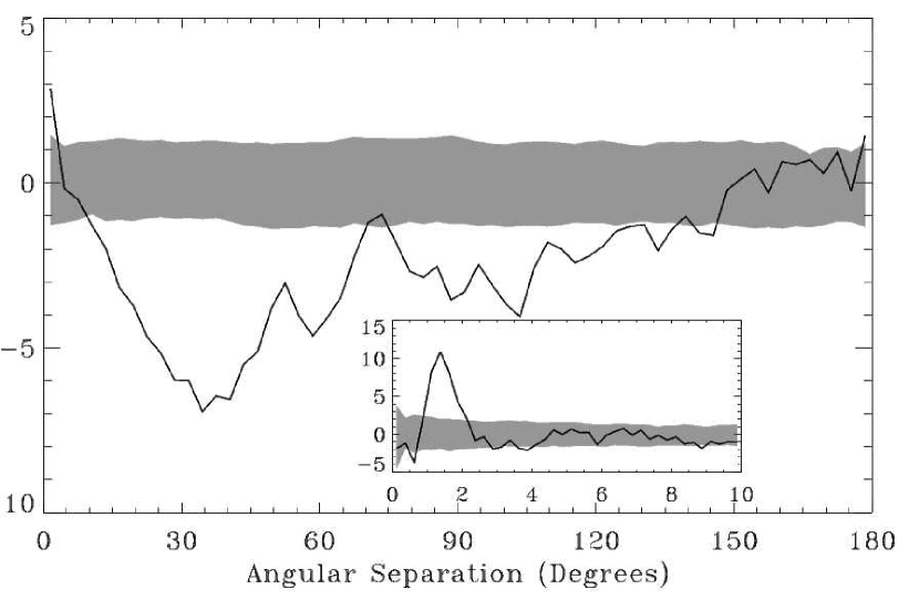
Figure 2: Temperature-polarization correlation function for WMAP co-added QVW data. The gray band shows the 68% confidence interval for similar co-added data taken from Monte Carlo simulations without polarization. The inset shows data for $\theta<10\arcdeg$. The data are inconsistent with no temperature-polarization cross-correlations at more than 10 standard deviations. Note that the data are not independent between angular bins.

The Microwave Anisotropy Probe has mapped the full sky in the Stokes $I$, $Q$, and $U$ parameters on angular scales $\theta>0\fdg 2$ in 5 frequency bands centered at 23, 33, 41, 61, and 94 GHz (Bennett et al., 2003a). WMAP was not designed solely as a polarimeter, in the sense that none of its detectors are sensitive only to polarization. Incident radiation in each differencing assembly (DA) is split by an orthomode transducer (OMT) into two orthogonal linear polarizations (Page et al., 2003b; Jarosik et al., 2003). Each OMT is oriented so that the electric field directions accepted in the output rectangular waveguides lie at $\pm 45\arcdeg$ with respect to the $yz$ symmetry plane of the satellite (see Bennett et al. (2003a) Fig. 2 for the definition of the satellite coordinate system). The two orthogonal polarizations from the OMT are measured by two independent radiometers. Each radiometer differences the signal in the accepted polarization between two positions on the sky (the A and B beams), separated by $\sim 140\arcdeg$.

The signal from the sky in each direction $\hat{n}$ can be decomposed into the Stokes parameters

$$T(\hat{n})=I(\hat{n})+Q(\hat{n})\cos{2\gamma}+U(\hat{n})\sin{2\gamma},$$ (1)

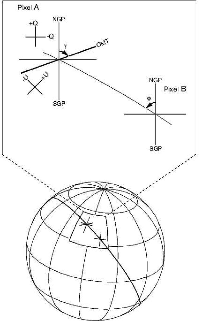
Figure 1: Geometry for Stokes $Q$ and $U$ parameters. WMAP measures polarization by differencing two orthogonal polarization channels, then solving for $Q$ and $U$ as the spacecraft compound spin projects the OMT onto the sky at different angles $\gamma$ relative to the Galactic meridians. All analysis uses coordinate-independent quantities $Q^{\prime}$ and $U^{\prime}$ defined with respect to the great circle connecting a pair of pixels (see text).

where we define the angle $\gamma$ from a meridian through the Galactic poles to the projection on the sky of the E-plane of each output port of the OMT (Fig. 1). In principle, by tracking the orientation of the OMTs on the sky as the satellite scan pattern observes each sky pixel in different orientations, each radiometer could independently produce a map of the Stokes $I$, $Q$, and $U$ parameters. In practice, the non-uniform coverage of $\gamma$ at each pixel would generate significant correlations between the fitted Stokes parameters, allowing leakage of the dominant temperature anisotropy into the much fainter polarization maps. We avoid this problem by differencing the outputs of the two radiometers in each differencing assembly in the time-ordered data. Denoting the two radiometers by subscripts 1 and 2, the instantaneous outputs are

$$\Delta T_{1} = I(\hat{n}_{A})+Q(\hat{n}_{A})\cos 2\gamma_{A}+U(\hat{n}_{A})\sin 2\gamma_{A}$$ (2)

$$- I(\hat{n}_{B})-Q(\hat{n}_{B})\cos 2\gamma_{B}-U(\hat{n}_{B})\sin 2\gamma_{B}$$

and

$$\Delta T_{2} = I(\hat{n}_{A})-Q(\hat{n}_{A})\cos 2\gamma_{A}-U(\hat{n}_{A})\sin 2\gamma_{A}$$

$$- I(\hat{n}_{B})+Q(\hat{n}_{B})\cos 2\gamma_{B}+U(\hat{n}_{B})\sin 2\gamma_{B}.$$

The sum

$$\Delta T_{I}\equiv\frac{1}{2}(\Delta T_{1}+\Delta T_{2})=I(\hat{n}_{A})-I(\hat{n}_{B})$$ (3)

is thus proportional to the unpolarized intensity, while the difference

$$\Delta T_{P}\equiv\frac{1}{2}(\Delta T_{1}-\Delta T_{2})=Q(\hat{n}_{A})\cos 2\gamma_{A}+U(\hat{n}_{A})\sin 2\gamma_{A}-Q(\hat{n}_{B})\cos 2\gamma_{B}-U(\hat{n}_{B})\sin 2\gamma_{B}.$$ (4)

is proportional only to the polarization. We produce full-sky maps of the Stokes $I$, $Q$, and $U$ parameters from the sum and difference time-ordered data using an iterative mapping algorithm. Since the polarization is faint, the $Q$ and $U$ maps are dominated by instrument noise and converge rapidly (Hinshaw et al., 2003a).

The Stokes $Q$ and $U$ components depend on a specific choice of coordinate system. For each pair of pixels, we define coordinate-independent quantities

$$Q^{\prime}=Q\cos(2\phi)+U\sin(2\phi)$$

$$U^{\prime}=U\cos(2\phi)-Q\sin(2\phi),$$ (5)

where the angle $\phi$ rotates the coordinate system about the outward-directed normal vector to put the meridian along the great circle connecting the two positions on the sky (Kamionkowski et al., 1997; Zaldarriaga & Seljak, 1997). All of our analyses use these coordinate-independent linear combinations of the $Q$ and $U$ sky maps.

Simulations of the mapping algorithm demonstrate that WMAP can accurately recover the polarization pattern on the sky, even after allowing for residual calibration uncertainty in the individual radiometer channels. However, non-ideal instrumental signals affect the $Q$ and $U$ sky maps to a greater extent than the unpolarized $I$ maps. The spacecraft spin about its $z$ axis sweeps the beams across the sky in a direction $45\arcdeg$ from the OMT orientation, preferentially coupling signals not fixed on the sky into the $U$ map. Residual striping exists to a lesser extent in the $I$ and $Q$ maps. Systematic errors in the individual $Q$ and $U$ maps are not yet fully assessed; consequently, we defer detailed analysis of the $Q$ or $U$ maps to a later paper. Cross-correlations between maps are largely unaffected by striping or any other channel-specific signal, allowing much simpler analysis of the faint polarization signal than would be possible for the individual $Q$ or $U$ maps. This paper discusses the temperature-polarization (TE) correlation in the WMAP one-year sky maps.

We compute the temperature-polarization cross-correlation using three different techniques: the two-point correlation function, a quadratic estimator for the power spectrum, and a “template” comparison in pixel space between the polarization maps and the predicted polarization given the observed pattern of temperature anisotropy. All three methods yield similar results despite disparate treatments of the data.

2 CORRELATION FUNCTION

The simplest measure of temperature-polarization cross-correlation is the two-point angular correlation function

$$C^{IQ}(\theta)=\frac{\sum_{ij}I_{i}Q^{\prime}_{j}w_{i}w_{j}}{\sum_{ij}w_{i}w_{j}},$$ (6)

where $i$ and $j$ are pixel indices and $w$ are the weights. To avoid possible effects of $1/f$ noise, we force the temperature map to come from a different frequency band than the polarization maps, and thus use the temperature map at 61 GHz (V band) for all correlations except the V-band polarization maps, which we correlate against the 41 GHz (Q band) temperature map. Since WMAP has a high signal-to-noise ratio measurement of the CMB temperature anisotropy, we use unit weight ($w_{i}=1$) for the temperature maps and noise weight ($w_{j}=N_{j}/\sigma_{0}^{2}$) for the polarization maps, where $N_{j}$ is the effective number of observations in each pixel $j$ and $\sigma_{0}$ is the standard deviation of the white noise in the time-ordered data (Table 1 of Bennett et al. (2003b)). We compare the correlation functions to Monte Carlo simulations of a null model, which simulates the temperature anisotropy using the best-fit $\Lambda$CDM model (Spergel et al., 2003) but forces the polarization signal to zero. Each realization generates a CMB sky in Stokes $I$, $Q$, and $U$ parameters, convolves this simulated sky with the beam pattern for each differencing assembly, then adds uncorrelated instrument noise to each pixel in each map. We then co-add the simulated skies in each frequency band and compute $C^{IQ}(\theta)$ using the same software for both the WMAP data and the simulations. All analysis uses only pixels outside the WMAP Kp0 foreground emission mask (Bennett et al., 2003c), approximately 76% of the full sky.

Figure 2 shows $C^{IQ}(\theta)$ derived by co-adding the individual correlation functions for the frequencies 41, 61, and 94 GHz (Q, V, and W bands) least likely to be affected by Galactic foregrounds. The grey band shows the 68% confidence interval for the null simulations. It is clear that WMAP detects a temperature-polarization signal at high statistical confidence, and that signals exist on both large and small angular scales. We define a goodness-of-fit statistic

$$\chi^{2}=\sum_{ab}~{}[C^{IQ}_{\rm MAP}-\langle C^{IQ}_{\rm sim}\rangle]_{a}~{}{\bf M}^{-1}_{ab}~{}[C^{IQ}_{\rm MAP}-\langle C^{IQ}_{\rm sim}\rangle]_{b},$$ (7)

where $C^{IQ}_{\rm MAP}$ is the co-added correlation function from WMAP data, $\langle C^{IQ}_{\rm sim}\rangle$ is the mean from the Monte Carlo simulations, and ${\bf M}$ is the covariance matrix between angular bins $a$ and $b$ derived from the simulations. We find $\chi^{2}=207$ for 78 degrees of freedom when comparing WMAP to the null model: WMAP detects temperature-polarization correlations significant at more than 10 standard deviations.

2.1 Systematic Error Analysis

Having detected a significant signal in the data, we must determine whether this signal has a cosmological origin or results from systematic errors or foreground sources. We test the convergence of the mapping algorithm using end-to-end simulations, comparing maps derived from simulated time-ordered data to the input maps used to generate the simulated time series. The simulations include all major instrumental effects, including beam ellipticity, radiometer performance, and instrument noise (including $1/f$ component), and are processed using the same map-making software as the WMAP data (Hinshaw et al., 2003a). The $Q$ and $U$ maps converge rapidly, within the 30 iterations required to derive the calibration solution. Correlations in the time-ordered data introduce an anti-correlation in the $U$ map at angles corresponding to the beam separation, with amplitude 0.5% of the noise in the map. This effect is independent for each radiometer and does not affect temperature-polarization cross-correlations. Similarly, residual $1/f$ noise in the time series can create faint striping in the maps, but does not affect cross-correlations.

The largest potential systematic error in the temperature-polarization cross-correlation results from bandpass mismatches in the amplification/detection chains. We calibrate the WMAP data in thermodynamic temperature using the Doppler dipole from the satellite’s orbit about the Sun as a beam-filling calibration source (Hinshaw et al., 2003a). Astrophysical sources with a spectrum other than a 2.7 K blackbody are thus slightly mis-calibrated. The amplitude is dependent on the product of the source spectrum with the unique bandpass of each radiometer. If the bandpasses in each radiometer were identical, the effect would cancel for any frequency spectrum, but differences in the bandpasses between the two radiometers in each DA generate a non-zero residual in the difference signal used to generate polarization maps (Eq. 4). This signal is spatially correlated with the unpolarized foreground intensity but is independent of the orientation of the radiometers on the sky (polarization angle $\gamma$). In the limit of uniform sampling of $\gamma$ this term drops out of the sky map solution. However, the WMAP scan pattern does not view each pixel in all orientations; unpolarized emission with a non-CMB spectrum can thus be aliased into polarization if the bandpasses of the two radiometers in each DA are not identical. This is a significant problem only at 23 GHz (K band), where the foregrounds are brightest and the bandpass mismatch is largest.

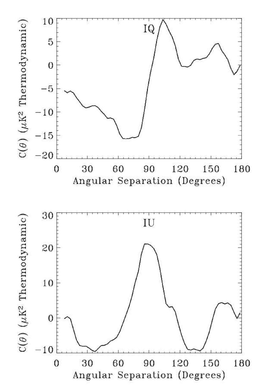
Figure 3: Angular templates for potential systematic errors caused by bandpass mismatch between the 2 radiometers in each differencing assembly. We fit this template to the correlation functions from each DA to detect or limit systematic errors related to bandpass mismatch in the main beam. The effect is significant only in K and Ka bands, which have the brightest unpolarized foregrounds.

We quantify the effect of bandpass mismatch using end-to-end simulations. For each time-ordered sample, we compute the signal in each radiometer using an unpolarized foreground model and the measured pass bands in each output channel (Jarosik et al., 2003). We then generate maps from the simulated data using the WMAP one-year sky coverage and compute $C^{IQ}(\theta)$ using the output $I$, $Q$, and $U$ maps from the simulation. Figure 3 shows the predicted signal at K band. We treat this as an angular template and compute the least-squares fit of the WMAP data to this bandpass template to determine the amplitude of the effect in the observed correlation functions. We correct the WMAP correlation functions $C^{IQ}(\theta)$ and $C^{IU}(\theta)$ at K and Ka bands by subtracting the best-fit template amplitudes. The fitted signal has peak amplitude of 8 $\mu$K² at 23 GHz and 5 $\mu$K² at 33 GHz. No other channel has a statistically significant detection of this effect.

Sidelobe pickup of polarized emission from the Galactic plane can also produce spurious polarization at high latitudes in the $Q$ and $U$ maps. We estimate this effect using the measured far-sidelobe response for each beam in each polarization (Barnes et al., 2003). The simplest approach would be to estimate the signal in each time-ordered sample, convolving the full sky sidelobe response with the Stokes $I$, $Q$, and $U$ maps given the instantaneous orientation of the beams for each sample. Such an approach is computationally expensive. We instead approximate the signal in each pixel by convolving the full sky sidelobe response with the one-year $Q$ and $U$ maps. For each pixel, we fix one beam on that pixel while sweeping the other beam through all orientations achieved in flight. The average from the convolution yields the sidelobe contribution for the pixel in question. Details of the sidelobe maps are presented in Barnes et al. (2003). We correlate the sidelobe maps with the temperature anisotropy maps in each channel to estimate the systematic error in the temperature-polarization correlation. Sidelobe pickup of polarized structure in the Galactic plane is less than 1 $\mu$K² in $C^{IQ}(\theta)$ at 23 GHz and below 0.1 $\mu$K² in all other bands. The effect of bandpass mismatch in the far sidelobes (as opposed to the main beam) is similarly weak, with limits 1.3 $\mu$K² at 23 GHz and less than 0.05 $\mu$K² in all other bands. We correct the polarization maps for the estimated sidelobe signal and propagate the associated systematic uncertainty throughout our analysis. Note that all of these systematic errors depend on the Galactic foregrounds, and have different frequency dependence than CMB polarization.

Other instrumental effects are negligible. We measure polarization by differencing the outputs of the two radiometers in each differencing assembly (Eq. 4). Calibration errors (as opposed to the bandpass effect discussed above) can alias temperature anisotropy into a spurious polarization signal. We have simulated the uncertainty in the calibration solution using both realistic gain drifts and drifts ten times larger than observed in flight (Hinshaw et al., 2003a). Gain drifts (either intrinsic or thermally-induced) contribute less than 1 $\mu$K² to $C^{IQ}(\theta)$ in the worst band.

Null tests provide an additional check for systematic errors. Thomson scattering of scalar temperature anisotropy produces a curl-free polarization pattern. A non-zero cosmological signal is thus expected only for the IQ (TE) correlation, whereas systematic errors or foreground sources can affect both the IQ and IU (TB) correlations. We also test linear combinations of radiometer maps which cancel the polarization signal but which test for systematic effects. We compute the IQ and IU correlation functions by correlating the Stokes $I$ sum map from the Q- or V-band (as noted above) with the polarization difference maps $(Q1-Q2)/2$, $(V1-V2)/2$, $(W1-W2)/2$, and $(W3-W4)/2$. We then co-add the results with their noise weights, and compare the co-added result for the polarization difference maps to a similar computation for the polarization sum maps. The temperature (Stokes $I$) map in all cases is a sum map; the test is thus primarily sensitive to systematic errors in the polarization data.

Table 1 shows results of the null tests. We compare $C^{IQ}(\theta)$ and $C^{IU}(\theta)$ for the sum and difference maps to a null hypothesis that the data consist of Stokes $I$ and instrument noise, with no polarization in the Stokes $Q$ or $U$ maps. We break the data into 2 angular regimes to differentiate between signals at decoupling vs reionization. We find a clear signal detection for $C^{IQ}(\theta)$ in the sum map for both angular scales. All other tests are consistent with instrument noise – there is no evidence for additional systematic errors in the temperature-polarization cross-correlation.

2.2 Foregrounds

Galactic emission is not a strong contaminant for CMB temperature anisotropy, but could be significant in polarization. WMAP measurements of unpolarized foreground emission show synchrotron, free-free, and thermal dust emission all sharing significant spatial structure (Bennett et al., 2003c). Of these components, only synchrotron emission is expected to generate significant polarization; other sources such as spinning dust are limited to less than 5% of the total intensity at 33 GHz.

Synchrotron emission from electrons accelerated in the Galactic magnetic field is the dominant unpolarized foreground at frequencies below $\sim$50 GHz. Although it is known to be linearly polarized, previous radio surveys provide little guidance for the high-latitude polarization at mm wavelengths. Extrapolation of radio polarization maps (Brouw & Spoelstra, 1976) to millimeter wavelengths indicate a polarization fraction between 10% and 50% depending on Galactic latitude (Lubin & Smoot, 1981). The unpolarized component has angular power spectrum $c_{\ell}\propto\ell^{-2}$, while the CMB power spectrum rises to a set of peaks on angular scales $\theta\approx 1\arcdeg$ (cf Fig 10(b) of Bennett et al. (2003c)). The angular dependence of the polarized foreground component is expected to be even steeper (Baccigalupi et al., 2001; Bruscoli et al., 2002; Tucci et al., 2002), suggesting that foreground polarization is most likely to affect temperature-polarization correlations on large angular scales. Radio maps at low Galactic latitude, however, demonstrate that the polarization intensity is not necessarily well correlated with the unpolarized intensity, complicating template analysis for temperature-polarization cross-correlations (Uyanıker et al., 1998, 1999). We thus use the frequency dependence of the measured temperature-polarization cross-correlation to separate cosmic from foreground signals.

Foreground polarization above 40 GHz is faint: fitting the correlation functions at 41, 61, and 94 GHz (Q, V, and W bands) to a single power-law $C^{IQ}(\theta,\nu)=C_{0}^{IQ}(\theta)~{}(\nu/\nu_{0})^{\beta}$ yields spectral index $\beta=-0.4\pm 0.4$, consistent with a CMB signal ($\beta=0$) and inconsistent with the spectral indices expected for synchrotron ($\beta\approx-3$), spinning dust ($\beta\approx-2$), or thermal dust ($\beta\approx 2$). The measured signal can not be produced solely by a single foreground emission component (unless the fractional polarization of the foreground emission has a compensating frequency dependence, which seems unlikely).

A two-component fit

$$C^{IQ}(\theta,\nu)=C_{\rm CMB}^{IQ}(\theta)~{}+~{}C_{\rm Gal}^{IQ}(\theta)\left(\frac{\nu}{\nu_{0}}\right)^{\beta}$$ (8)

tests for the superposition of a CMB component with a single foreground component. Figure 4 shows the resulting decomposition into CMB and foreground components. We obtain a marginal detection of foreground component with best-fit spectral index $\beta=-3.7\pm 0.8$ consistent with synchrotron emission. We test for consistency or possible residual systematic errors by repeating the fit using different temperature maps and different combinations of WMAP polarization channels. The fitted CMB component (left panels of Fig. 4) is robust against all combinations of frequency channels and fitting techniques. Note the agreement in Fig. 4 between nearly independent data sets: the co-added QVW data (uncorrected for foreground emission) and the KKaQ data (corrected for foreground emission). We obtain additional confirmation by replacing the V-band temperature map in the cross-correlation (Eq. 6) with the “internal linear combination” temperature map designed to suppress foreground emission (Bennett et al., 2003c). The fitted CMB component does not change. We test for systematic errors by replacing the temperature map with the COBE-DMR map of the CMB temperature (Bennett et al., 1996), excluding any instrumental correlation between the temperature and polarization data. Again, the results are unchanged.

We further constrain foreground contributions by computing the cross-correlation between the WMAP polarization data and temperature maps dominated by foregrounds. We replace the temperature map in Eq. 6 with either the WMAP maximum-entropy foreground model (Bennett et al., 2003c) or a “residual” foreground map created by subtracting the internal linear combination CMB map from the individual WMAP temperature maps. We then correlate the foreground temperature map against the WMAP polarization data in each frequency band, and fit the resulting correlation functions to CMB and foreground components (Eq. 8). The two foreground maps provide nearly identical results. The fitted CMB component has nearly zero amplitude, consistent with the instrument noise. The fitted foreground has amplitude $0.5\pm 0.1~{}\mu$K² at $\nu_{0}$ = 41 GHz, with best-fit index $\beta=-3.4$ consistent with synchrotron emission.

3 POLARIZATION CROSS-POWER SPECTRA

In a second analysis method, we compute the angular power spectrum of the temperature-polarization correlations using a quadratic estimator (Appendix A). The power spectrum is the Legendre transform of the two-point correlation function, and is more commonly encountered for theoretical predictions. We compute $c_{l}^{TE}$ and $c_{l}^{TB}$ individually for the each WMAP frequency band, using uniform weight for the temperature map and noise weight for the polarization maps. We then combine the angular power spectra, using noise-weighted QVW data for $l>21$ where foregrounds are insignificant, and a fit to CMB plus foregrounds using all 5 frequency bands for $l\leq 21$. Since foreground contamination is weak, we gain additional sensitivity in this analysis by using the Kp2 sky cut retaining 85% of the sky.

We estimate the uncertainty in each $l$ bin using the covariance matrix ${\bf M}$ for the polarization cross-power spectrum. Based on our analysis of the $c_{l}^{TT}$ covariance matrix (Hinshaw et al., 2003b), the $c_{l}^{TE}$ covariance matrix has the form along the diagonal of

$${\bf M}_{ll} = <c_{l}^{TE}c_{l}^{TE}>-<c_{l}^{TE}>^{2}$$ (10)

$$\simeq\frac{(c_{l}^{TT}+n_{TT}/w_{l})(c_{l}^{EE}+n_{EE}/w_{l})+(c_{l}^{TE})^{2}}{(2l+1)f_{sky}f_{sky}^{\rm eff}}$$

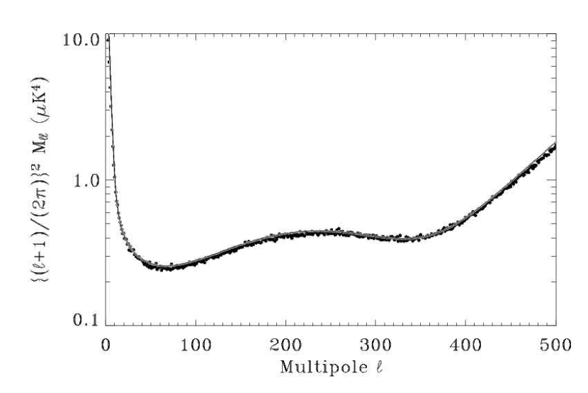
Figure 5: Diagonal elements of the covariance matrix for the $c_{l}^{TE}$ polarization cross-power spectrum. Points show the diagonal elements computed from 7500 Monte Carlo simulations. The solid line shows the analytical model (Eq. 10). Note we multiply ${\bf M}_{ll}$ by $\left(\frac{l+1}{2\pi}\right)^{2}$ to match the units in Figures 7 and 8.

where $n_{TT}$ and $n_{EE}$ are the TT and EE noise bias terms, $w_{l}$ is the effective window function for the combined maps (Page et al., 2003a), $c_{l}^{TT}$ and $c_{l}^{EE}$ are the temperature and polarization angular power spectra, $f_{sky}=0.85$ is the fractional sky coverage for the Kp2 mask, and $f_{sky}^{\rm eff}=f_{sky}/1.14$ for noise weighting. We take the $c_{l}^{TT}$ term from the measured temperature power spectra (Hinshaw et al., 2003b) and the $c_{l}^{EE}$ term predicted by the best-fit $\Lambda$CDM model (Spergel et al., 2003) (allowing $c_{l}^{EE}$ to vary as a function of optical depth in the likelihood analysis). Figure 5 compares the analytic expression for the diagonal elements of the covariance matrix to the mean derived from 7500 Monte Carlo simulations. The analytic form (Eq. 10) accurately describes the simulations. We approximate the off-diagonal terms using the geometric mean of the covariance matrix terms for uniform and noise weighting (Hinshaw et al., 2003b),

$${\bf M}_{ll^{\prime}}\simeq(~{}{\bf M}_{ll}{\bf M}_{l^{\prime}l^{\prime}}~{})^{0.5}~{}r_{\Delta l}.$$ (11)

Figure 6 shows the off-diagonal terms $r_{\Delta l}$ measured from Monte Carlo simulations. The largest contribution, $-2.8\%$, is at $\Delta l=2$ from the symmetry of our sky cut and noise coverage. The total anticorrelation is $\sum_{\Delta l\neq 0}r_{\Delta l}=-0.124$. Because of this anti-correlation, the error bars for the binned $c_{l}^{TE}$ are slightly smaller than the naive estimate. A second method of estimating the errors relies on end-to-end simulations derived from simulated time-ordered data consisting solely of instrument noise (including the estimated contribution from $1/f$ fluctuations). We have generated 11 “noise” sky maps each in Stokes $I$, $Q$, and $U$ and compute the variance in TE directly from the variance in the simulated signal. These two approaches yield errors that are consistent to better than 5%. Since there are $2l+1$ multipoles at each $l$ value, the fractional uncertainty expected in the Monte Carlo variance is $[2/(11(2l+1)f_{sky})]^{0.5}$, in agreement with this result.

Figure 7 shows the polarization cross-power spectra for the WMAP one-year data. The solid line shows the predicted signal for adiabatic CMB perturbations, based only on a fit to the measured temperature angular power spectrum $c_{l}^{TT}$ (Spergel et al., 2003; Hinshaw et al., 2003b). Two features are apparent. The TE data on degree angular scales ($l>20$) are in excellent agreement with a priori predictions of adiabatic models (Coulson et al., 1994). Other than the specification of adiabatic perturbations, there are no free parameters – the solid line is not a fit to $c_{l}^{TE}$. The $\chi^{2}$ of 24.2 for 23 degrees of freedom indicates that the CMB anisotropy is dominated by adiabatic perturbations. On large angular scales ($l<20$) the data show excess power compared to adiabatic models, suggesting significant reionization.

The WMAP detection of the acoustic structure in the TE spectrum confirms several basic elements of the standard paradigm. The amplitudes of the peak and anti-peak are a measure of the thickness of the decoupling surface, while the shape confirms the assumption that the primordial fluctuations are adiabatic. Adiabatic fluctuations predict a temperature/polarization signal anticorrelated on large scales, with TE peaks and anti-peaks located midway between the temperature peaks Hu & Sugiyama (1994). The existence of TE correlations on degree angular scales also provides evidence for super-horizon temperature fluctuations at decoupling, as expected for inflationary models of cosmology (Peiris et al., 2003)

4 TEMPLATE POWER SPECTRA

Figure 7 demonstrates that the power spectrum of temperature-polarization correlations on degree angular scales can be predicted using the power spectrum of the temperature fluctuations alone. We use this for a third derivation of the TE cross-power spectrum, based on template matching in pixel space. For pixel sizes of a few degrees, the signal-to-noise ratio for the temperature maps is much larger than one per multipole, while the S/N ratio in the polarization maps is much less than one. The likelihood function for the polarization measurement then has the simple form

$$\log{\cal L}=(\hat{P}-\sum_{l}\alpha_{l}\hat{P}_{\rm pred}^{l})^{T}N^{-1}(\hat{P}-\sum_{l}\alpha_{l}\hat{P}_{\rm pred}^{l}),$$ (12)

where $\hat{P}$ is the measured polarization signal (a 2 $N_{\rm pixel}$ vector), $\alpha_{l}=c_{l}^{TE}/c_{l}^{TT}$ is the polarization fraction at each $l$, $N$ is the pixel noise correlation matrix (a $2N_{\rm pixel}\times 2N_{\rm pixel}$ matrix) and

$$Q_{pred}^{l}(\hat{n})=\sum_{m}a_{lm}(_{2}Y_{lm}(\hat{n})+_{-2}Y_{lm}(\hat{n}))$$

$$U_{pred}^{l}(\hat{n})=i\sum_{m}a_{lm}(_{2}Y_{lm}(\hat{n})-_{-2}Y_{lm}(\hat{n})).$$ (13)

Here ${}_{\pm 2}Y_{lm}(\hat{n})$ are the spin harmonics, while $a_{lm}$ are the measured coefficients for an all-sky map of the CMB temperature. Imposing a cut to mask the Galactic plane introduces additional correlations; we avoid this by using the “internal” linear combination temperature map (Bennett et al., 2003c) without imposing a sky cut.

The maps $Q_{pred}$ and $U_{pred}$ represent the predicted polarization pattern based on the observed pattern of temperature anisotropy. We fit these template maps to the observed $Q$ and $U$ polarization maps to derive the polarization fraction $\alpha_{l}$ and thus the $c_{l}^{TE}$ polarization cross-power spectrum. Minimizing the likelihood function yields the normal equations

$$K_{ll^{\prime}}\alpha_{l^{\prime}}=y_{l},$$ (14)

where

$$y_{l}=\hat{P}N^{-1}\hat{P}_{pred}^{l}$$ (15)

and

$$K_{ll^{\prime}}=\hat{P}_{pred}^{l}N^{-1}\hat{P}_{pred}^{l^{\prime}}.$$ (16)

These equations show the advantages of this approach. We compare the data with a template in pixel space, making it straightforward to include a spatially varying noise signal. We directly compare the measured polarization maps to a prediction based on the measured temperature maps, yielding a measurement of the TE polarization cross-power spectrum in the observed sky unaffected by cosmic variance. We can thus more easily compute the errors on the measured polarization fraction. The input temperature map (Stokes $I$) is already corrected for foreground emission (much simpler in pixel space where the unpolarized foregrounds are more easily measured), greatly reducing the foreground contribution to the cross-power spectra.

We thus compute the temperature-polarization cross-correlation using three disparate techniques: the two-point angular correlation function, a quadratic estimator for the power spectrum in Fourier space, and a template fit in pixel space. All methods are in good agreement despite their very dissimilar treatment of the data. All methods show a significant excess of power for $l<10$.

5 REIONIZATION

WMAP detects statistically significant correlations between the CMB temperature and polarization. The signal on degree angular scales ($l>20$) agrees with the signal expected in adiabatic models based solely on the temperature power spectrum, without any additional free parameters. We also detect power on large angular scales ($l<10$) well in excess of the signal predicted by the temperature power spectrum alone. This signal can not be explained by data processing, systematic errors, or foreground polarization, and has a frequency spectrum consistent with a cosmological origin.

The signal on large angular scales has a natural interpretation as the signature of early reionization. Both the temperature and temperature-polarization power spectra can be related to the power spectrum of the radiation field during scattering (Zaldarriaga, 1997). Thomson scattering damps the temperature anisotropy and regenerates a polarized signal on scales comparable to the horizon. The existence of polarization on scales much larger than the acoustic horizon at decoupling implies significant scattering at more recent epochs.

5.1 Reionization in a $\Lambda$CDM Universe

If we assume that the $\Lambda$CDM model is the best description of the physics of the early universe, we can fit the observed temperature-polarization cross-power spectrum to derive the optical depth $\tau$. We assume a step function for the ionization fraction $x_{e}$ and use the CMBFAST code (Seljak & Zaldarriaga, 1996) to predict the multipole moments as a function of optical depth. While this assumption is simplistic, our conclusions on optical depth are not very sensitive to details of the reionization history or the background cosmology.

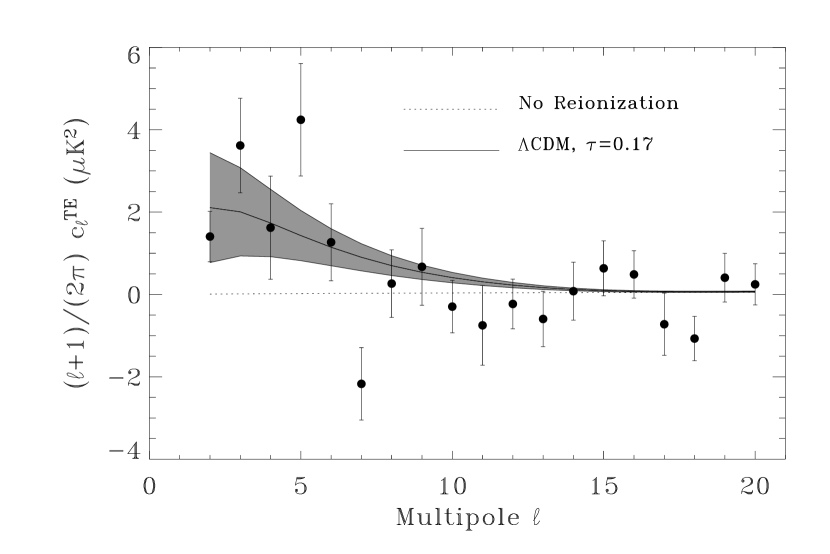
Figure 8: WMAP Polarization cross-power spectra $c_{\ell}^{TE}$ (filled circles) compared to $\Lambda$CDM models with and without reionization. The rise in power for $l<10$ is consistent with reionization optical depth $\tau=0.17\pm 0.04$. The error bars on WMAP data reflect measurement errors only; adjacent points are slightly anti-correlated. The grey band shows the 68% confidence interval from cosmic variance. The value at $l=7$ is particularly sensitive to the foreground correction.

Figure 8 compares the polarization cross-power spectrum $c_{l}^{TE}$ derived from the quadratic estimator to $\Lambda$CDM models with and without reionization. The rise in power for $l<10$ is clearly inconsistent with no reionization. We quantify this using a maximum-likelihood analysis

$${\cal L}\propto\frac{\exp(-\frac{1}{2}\chi^{2})}{|{\bf M}|^{1/2}}.$$ (17)

Figure 9 shows the relative likelihood ${\cal L}/{\rm Max}({\cal L})$ for the optical depth $\tau$ assuming a $\Lambda$CDM cosmology, with all other parameters fixed at the values derived from the temperature power spectrum alone (Spergel et al., 2003). The likelihood for the 5-band data corrected for foreground emission peaks at $\tau=0.17\pm 0.03$ (statistical error only): WMAP detects the signal from reionization at high statistical confidence.

A full error analysis for $\tau$ must account for systematic errors and foreground uncertainties. We propagate these effects by repeating the maximum likelihood analysis using different combinations of WMAP frequency bands and different systematic error corrections. We correct $C^{IQ}(\theta)$ in each frequency band not for the best estimate of the systematic error templates, but rather the best estimate plus or minus one standard deviation. We then fit the mis-corrected $C^{IQ}(\theta,\nu)$ for a CMB piece plus a foreground piece (Eq. 8) and use the CMB piece in a maximum-likelihood analysis for $\tau$. The change in the best-fit value for $\tau$ as we vary the systematic error corrections propagates the uncertainties in these corrections. Systematic errors have a negligible effect on the fitted optical depth; altering the systematic error corrections changes the best-fit values of $\tau$ by less than 0.01.

The largest non-random uncertainty is the foreground separation. We assess the uncertainty in the foreground separation by repeating the entire systematic error analysis (using both standard and altered systematic error corrections) with the foreground spectral index $\beta=-3.7\pm 0.8$ shifted one standard deviation up or down from the best-fit value. Table 2 shows the fitted optical depth $\tau$ and goodness-of-fit statistic $\chi^{2}$ for different data combinations and foreground spectral indices derived from the analysis of the two-point correlation function $C^{IQ}(\theta)$. The first set of rows shows values derived by simply co-adding the WMAP frequency channels, without any correction for foregrounds. Data at 41, 61, and 94 GHz (Q, V, and W bands) where foregrounds are negligible show similar values for $\tau$; the $\chi^{2}\approx 66$ for 57 degrees of freedom indicates that the data are in agreement with reionized models. Adding additional low-frequency channels reduces the formal statistical uncertainty, but introduces non-zero foreground contamination as shown by the marked increase in $\chi^{2}$. The next three sets of rows show the results when the data are separated into CMB and foreground components (Eq. 8). All data combinations are now in agreement; we obtain nearly identical values for $\tau$ when fitting either the highest-frequency data set QVW or the lowest-frequency set KKaQ. The fitted optical depth is insensitive to the spectral index: varying the spectral index from -2.9 to -4.5 changes the fitted values by 0.02 or less. We adopt $\tau=0.17\pm 0.04$ as the best estimate for the optical depth to reionization, where the error bar reflects a 68% confidence level interval including statistical, systematic, and foreground uncertainties.

Spergel et al. (2003) include the TE data in a maximum-likelihood analysis combining WMAP data with other astronomical measurements. The resulting value, $\tau=0.17\pm 0.06$, is consistent with the value derived from the TE data alone. The larger uncertainty reflects the effect of simultaneously fitting multiple parameters. The TE analysis propagates foreground uncertainties by re-evaluating the likelihood using different foreground spectral index. Since foreground affect only the lowest multipoles, the combined analysis propagates foreground uncertainty by doubling the statistical uncertainty in $c_{l}^{TE}$ for $2\leq l\leq 4$ to account for this effect.

5.2 Model-Independent Estimate

An alternative approach avoids assuming any cosmological model and uses the measured temperature angular correlation function to determine the radiation power spectrum at recombination. This approach assumes that the best estimate of the three dimensional radiation power spectrum is the measured angular power spectrum rather than a model fit to the angular power spectrum. Given the observed temperature power spectrum $c_{l}^{TT}$, we derive the predicted polarization cross-power spectrum $c_{l}^{TE}$ (§4), which we then fit to the observed TE spectrum as a function of optical depth $\tau$. We obtain $\tau=0.16\pm 0.04$, in excellent agreement with the value derived assuming a $\Lambda$CDM cosmology. We emphasize that the model-independent technique makes no assumptions about the cosmology. The fact that it agrees well with the best-fit model from the combined temperature and polarization data (Spergel et al., 2003) is an additional indication that the observed temperature-polarization correlations on large angular scales represent the imprint of physical conditions at reionization. The dependence on the underlying cosmology is small.

5.3 Early Star Formation

Reionization can also be expressed as a redshift $z_{r}$ assuming an ionization history. We consider two simple cases. For instantaneous reionization with ionization fraction $x_{e}=1$ at $z<z_{r}$, the measured optical depth corresponds to redshift $z_{r}=17\pm 3$. This conflicts with measurements of the Gunn-Peterson absorption trough in spectra of distant quasars, which show neutral hydrogen present at $z\approx 6$ (Becker, 2001; Djorgovski et al., 2001; Fan, 2002). Reionization clearly did not occur through a single rapid phase transition. However, since absorption spectra are sensitive to even small amounts of neutral hydrogen, models with partial ionization $x_{e}\lesssim 1$ can have enough neutral column density to produce the Gunn-Peterson trough while still providing free electrons to scatter CMB photons and produce large-scale polarization. Direct Gunn-Peterson observations only imply a neutral hydrogen fraction $\gtrsim$ 1% (Fan, 2002). Accordingly, we modify the simplest model to add a second transition: a jump from $x_{e}=0$ to $x_{e}=0.5$ at redshift $z_{r}$, followed by a second transition from $x_{e}=0.5$ to $x_{e}=1$ at redshift $z=7$. Fitting this model to the measured optical depth yields $z_{r}\approx 20$. In reality, reionization is more complicated than simple step transitions. Allowing for model uncertainty, the measured optical depth is consistent with reionization at redshift $11<z_{r}<30$, corresponding to times $100<t_{r}<400$ Myr after the Big Bang (95% confidence).

Extrapolations of the observed ionizing flux to higher redshift lead to predicted CMB optical depth between $0.04-0.08$ (Miralda-Escude, 2002), lower than our best fit values. The measured optical depth thus implies additional sources of ionizing flux at high redshift. An early generation of very massive (Pop III) stars could provide the required additional heating. Tegmark (1997) estimate that $10^{-3}$ of all baryons should be in collapsed objects by $z=30$. If these baryons form massive stars, they would reionize the universe. However, photons below the hydrogen ionization threshold will destroy molecular hydrogen (the principal vehicle for cooling in early stars), driving the effective mass threshold for star formation to $\sim 10^{8}$ solar masses and impeding subsequent star formation (Haiman et al., 1997; Gnedin & Ostriker, 1997; Tegmark, 1997). X-ray heating and ionization (Venkatesan et al., 2001; Oh, 2001) may provide a loophole to this argument by enhancing the formation of $H_{2}$ molecules (Haiman et al., 2000).

Cen (2003) provides a physically-motivated model of “double reionization” that resembles the two-step model above. A first generation of massive Pop III stars initially ionizes the intergalactic medium. The increased metallicity of the intergalactic medium then produces a transition to smaller Pop II stars, after which the reduced ionizing flux allows regeneration of a neutral hydrogen fraction. The ionization fraction remains at $x_{e}\approx 0.6$ until the global star formation rate surpasses the recombination rate at $z=6$, restoring $x_{e}=1$. The predicted value $\tau=0.10\pm 0.03$ should be increased somewhat to reflect the higher WMAP values for the baryon density $\Omega_{b}$ and normalization $\sigma_{8}$ (Spergel et al., 2003). The contribution from ionized helium will also serve to increase $\tau$ (Venkatesan et al., 2003; Wyithe & Loeb, 2003). The WMAP determination of the optical depth indicates that ionization history must be more complicated than a simple instantaneous step function. While physically plausible models can reproduce the observed optical depth, reionization remains a complex process and can not be fully characterized by a single number. A more complete determination of the ionization history requires evaluation of the detailed $TE$ and $EE$ power spectra (Kaplinghat et al., 2003; Hu & Holder, 2003).

6 CONCLUSIONS

WMAP detects statistically significant correlations between the temperature and polarization maps. The correlations are inconsistent with instrument noise and are significantly larger than the upper limits established for potential systematic errors. The correlations are present in all WMAP frequency bands with similar amplitude from 23 to 94 GHz; fitting the data to a single power-law in frequency yields a spectral index $\beta=-0.4\pm 0.4$, consistent with a CMB signal ($\beta=0$) and inconsistent with the measured spectral indices for Galactic foreground emission. A two-component fit to a superposition of CMB and Galactic foregrounds yields a positive foreground detection in both curl- and curl-free modes, with best-fit spectral index $\beta=-3.7\pm 0.8$ consistent with synchrotron emission of amplitude $0.5\pm 0.1~{}\mu{\rm K}^{2}$ antenna temperature at 41 GHz.

The fitted CMB component is robust against different data combinations and fitting techniques. On small angular scales $(\theta<5\arcdeg)$, the WMAP data show the temperature-polarization expected from adiabatic perturbations in the temperature power spectrum. The data for $\ell>20$ agree well with the signal predicted solely from the temperature power spectra, with no additional free parameters.

The data show excess power on large angular scales ($\theta>10\arcdeg$) compared to the predictions based on the temperature power spectrum alone. The excess power is well described by early reionization at redshift $z_{r}=20^{+10}_{-9}$, corresponding to times $t_{r}=180^{+220}_{-80}$ Myr after the Big Bang (95% confidence). A model-independent fit to reionization optical depth yields results consistent with the $\Lambda$CDM model. Our best estimate for the optical depth is $\tau=0.17\pm 0.04$ (68% confidence) where the error terms include statistical, systematic, and foreground uncertainties. This value is larger than expected given the detection of a Gunn-Peterson trough in the absorption spectra of distant quasars, and implies that the universe has a complex ionization history.

The WMAP detection of early reionization opens a new frontier to explore the universe at redshift $6<z<30$. WMAP’s sensitivity to reionization is currently limited by instrument noise, both as direct statistical uncertainty and in the ability to better model and remove faint polarized foregrounds. Instrumental effects do not limit analysis of temperature-polarization correlations. The TE power spectrum and covariance matrix are available at http://lambda.gsfc.nasa.gov. We are currently performing a more complete set of systematic error analyses in the individual $Q$ and $U$ maps. A future data release will include full-sky polarization maps and polarization power spectra.

Appendix A Quadratic Estimator for Temperature-Polarization Power Spectrum

We estimate the temperature-polarization power spectrum from pixelized sky maps using the following formalism. We begin by expanding the temperature and polarization fluctuations in generalized spherical harmonics

$$T(\hat{n})=\sum_{lm}a_{lm}Y_{lm}(\hat{n})$$ (A1)

$$Q(\hat{n})\pm iU(\hat{n})=\sum_{lm}a_{\mp 2,lm}\ {}_{\mp 2}Y_{lm}(\hat{n})$$ (A2)

We then decompose the polarization fluctuations into $E$ and $B$ like pieces

$$a_{\pm 2,lm}=E_{lm}\pm iB_{lm}.$$ (A3)

We can use the basic properties of the spherical harmonics

$${}_{N}Y_{lm} = (-1)^{N}\ _{-N}Y_{l\ -m}^{*}$$ (A4)

$$\int d\hat{n}\ _{N}Y_{lm}(\hat{n})_{N}Y^{*}_{l^{\prime}m^{\prime}}(\hat{n}) = \delta_{l}^{l^{\prime}}\delta_{m}^{m^{\prime}}$$ (A5)

to derive

$$E_{lm}=\frac{1}{2}\int d\hat{n}~{} \left[~{}Q(\hat{n})\left(\ {}_{2}Y^{*}_{lm}(\hat{n})+\ _{-2}Y^{*}_{lm}(\hat{n})\right)\right.$$

$$-i\left.U(\hat{n})\left(\ {}_{2}Y^{*}_{lm}(\hat{n})-\ _{-2}Y^{*}_{lm}(\hat{n})\right)~{}\right]$$

$$B_{lm}=-\frac{1}{2}\int d\hat{n}~{} \left[~{}U(\hat{n})\left(\ {}_{2}Y^{*}_{lm}(\hat{n})+\ _{-2}Y^{*}_{lm}(\hat{n})\right)\right.$$ (A6)

$$+i\left.Q(\hat{n})\left(\ {}_{2}Y^{*}_{lm}(\hat{n})-\ _{-2}Y^{*}_{lm}(\hat{n})\right)~{}\right].$$

We can now generalize the approach of Hivon et al. (2002) to estimate the coupling terms. We multiply the temperature and polarization maps by a weighting function

$$\tilde{T}_{lm} = \int d\hat{n}~{}w^{T}(\hat{n})~{}T(\hat{n})Y^{*}_{lm}(\hat{n})$$ (A7)

$$\tilde{E}_{lm} = \frac{1}{2}\int d\hat{n}~{}w^{P}(\hat{n})~{}\left[Q(\hat{n})\left(\ {}_{2}Y^{*}_{lm}(\hat{n})+\ _{-2}Y^{*}_{lm}(\hat{n})\right)\right.$$ (A8)

$$\left.-iU(\hat{n})\ \left(\ {}_{2}Y^{*}_{lm}(\hat{n})-\ _{-2}Y^{*}_{lm}(\hat{n})\right)\right]$$

$$\tilde{B}_{lm} = -\frac{1}{2}\int d\hat{n}~{}w^{P}(\hat{n})~{}\left[U(\hat{n})\left(\ {}_{2}Y^{*}_{lm}(\hat{n})+\ _{-2}Y^{*}_{lm}(\hat{n})\right)\right.$$ (A9)

$$\left.+iQ(\hat{n})\left(\ {}_{2}Y^{*}_{lm}(\hat{n})-\ _{-2}Y^{*}_{lm}(\hat{n})\right)\right].$$

We expand the weighting function in spherical harmonics

$$w(\hat{n})=\sum_{lm}w_{lm}Y_{lm}(\hat{n}),$$ (A10)

and combine with equations A1 – A3 to yield

$$\tilde{T}_{lm} = \sum_{l^{\prime}m^{\prime}l^{\prime\prime}m^{\prime\prime}}w^{T}_{l^{\prime\prime}m^{\prime\prime}}T_{l^{\prime}m^{\prime}}\int d\hat{n}~{}Y_{l^{\prime}m^{\prime}}(\hat{n})Y_{l^{\prime\prime}m^{\prime\prime}}(\hat{n})Y^{*}_{lm}(\hat{n})$$

$$\tilde{E}_{lm} = \frac{1}{2}\sum_{l^{\prime}m^{\prime}l^{\prime\prime}m^{\prime\prime}}w^{P}_{l^{\prime\prime}m^{\prime\prime}}\left[E_{l^{\prime}m^{\prime}}\int d\hat{n}~{}Y_{l^{\prime\prime}m^{\prime\prime}}(\hat{n})\left(\ {}_{2}Y_{l^{\prime}m^{\prime}}(\hat{n})\ _{2}Y^{*}_{lm}(\hat{n})+\ _{-2}Y_{l^{\prime}m^{\prime}}(\hat{n})\ _{-2}Y^{*}_{lm}(\hat{n})\right)\right.$$

$$\left.+iB_{lm}\int d\hat{n}~{}Y_{l^{\prime\prime}m^{\prime\prime}}(\hat{n})\left(\ {}_{2}Y_{l^{\prime}m^{\prime}}(\hat{n})\ _{2}Y^{*}_{lm}(\hat{n})-\ _{-2}Y_{l^{\prime}m^{\prime}}(\hat{n})\ _{-2}Y^{*}_{lm}(\hat{n})\right)\right]$$

$$\tilde{B}_{lm} = \frac{1}{2}\sum_{l^{\prime}m^{\prime}l^{\prime\prime}m^{\prime\prime}}w^{P}_{l^{\prime\prime}m^{\prime\prime}}\left[B_{l^{\prime}m^{\prime}}\int d\hat{n}~{}Y_{l^{\prime\prime}m^{\prime\prime}}(\hat{n})\left(\ {}_{2}Y_{l^{\prime}m^{\prime}}(\hat{n})\ _{2}Y^{*}_{lm}(\hat{n})+\ _{-2}Y_{l^{\prime}m^{\prime}}(\hat{n})\ _{-2}Y^{*}_{lm}(\hat{n})\right)\right.$$ (A11)

$$\left.-iE_{lm}\int d\hat{n}~{}Y_{l^{\prime\prime}m^{\prime\prime}}(\hat{n})\left(\ {}_{2}Y_{l^{\prime}m^{\prime}}(\hat{n})\ _{2}Y^{*}_{lm}(\hat{n})-\ _{-2}Y_{l^{\prime}m^{\prime}}(\hat{n})\ _{-2}Y^{*}_{lm}(\hat{n})\right)\right].$$

We can then use

$$\int d\hat{n}\ _{N}Y_{lm}^{*}(\hat{n})\ _{N^{\prime}}Y_{l^{\prime}m^{\prime}}(\hat{n})\ _{N^{\prime\prime}}Y_{l^{\prime\prime}m^{\prime\prime}}(\hat{n}) = (-1)^{N+m}\left[\frac{(2l+1)(2l^{\prime}+1)(2l^{\prime\prime}+1)}{4\pi}\right]^{1/2}$$ (A16)

$$\left(\begin{array}[]{ccc}l&l^{\prime}&l^{\prime\prime}\\ -N&N^{\prime}&N^{\prime\prime}\end{array}\right)\left(\begin{array}[]{ccc}l&l^{\prime}&l^{\prime\prime}\\ -m&m^{\prime}&m^{\prime\prime}\end{array}\right)$$

to compute

$$\left(\begin{array}[]{c}\tilde{c}_{l}^{TT}\\ \tilde{c}_{l}^{TE}\\ \tilde{c}_{l}^{TB}\\ \tilde{c}_{l}^{EE}\\ \tilde{c}_{l}^{BB}\\ \end{array}\right)=\left(\begin{array}[]{ccccc}&&&&\\ &&&&\\ &&M_{ll^{\prime}}^{ab}&&\\ &&&&\\ &&&&\\ \end{array}\right)\left(\begin{array}[]{c}c_{l^{\prime}}^{TT}\\ c_{l^{\prime}}^{TE}\\ c_{l^{\prime}}^{TB}\\ c_{l^{\prime}}^{EE}\\ c_{l^{\prime}}^{BB}\\ \end{array}\right).$$ (A17)

These expressions can be reduced using the symmetry and orthogonality properties of 3-$j$ symbols, as given in Eqs. 1.8 and 1.14 of Rotenberg et al. (1959). In particular, imaginary terms drop out, and summations over products of 3-$j$ symbols with $-m$, $m^{\prime}$ and $m^{\prime\prime}$ in the bottom row evaluate to $1/(2l^{\prime\prime}+1)$. After some algebra, the coupling terms reduce to

$$M_{ll^{\prime}}^{TT,TT} = \frac{(2l^{\prime}+1)}{4\pi}\sum_{l^{\prime\prime}}{\cal W}^{TT}_{l^{\prime\prime}}\left(\begin{array}[]{ccc}l&l^{\prime}&l^{\prime\prime}\\ 0&0&0\end{array}\right)^{2}$$ (A20)

$$M_{ll^{\prime}}^{TE,TE} = M_{ll^{\prime}}^{TB,TB}$$ (A28)

$$=\frac{(2l^{\prime}+1)}{8\pi}\sum_{l^{\prime\prime}}{\cal W}^{TP}_{l^{\prime\prime}}\left(\begin{array}[]{ccc}l&l^{\prime}&l^{\prime\prime}\\ 0&0&0\end{array}\right)\left[\left(\begin{array}[]{ccc}l&l^{\prime}&l^{\prime\prime}\\ -2&2&0\end{array}\right)+\left(\begin{array}[]{ccc}l&l^{\prime}&l^{\prime\prime}\\ 2&-2&0\end{array}\right)\right]$$

$$M_{ll^{\prime}}^{EE,EE} = M_{ll^{\prime}}^{BB,BB}$$ (A39)

$$=\frac{(2l^{\prime}+1)}{16\pi}\sum_{l^{\prime\prime}}{\cal W}^{PP}_{l^{\prime\prime}}\left[\left(\begin{array}[]{ccc}l&l^{\prime}&l^{\prime\prime}\\ -2&2&0\end{array}\right)+\left(\begin{array}[]{ccc}l&l^{\prime}&l^{\prime\prime}\\ 2&-2&0\end{array}\right)\right]$$

$$\times\left[\left(\begin{array}[]{ccc}l&l^{\prime}&l^{\prime\prime}\\ -2&2&0\end{array}\right)+\left(\begin{array}[]{ccc}l&l^{\prime}&l^{\prime\prime}\\ 2&-2&0\end{array}\right)\right]$$

$$M_{ll^{\prime}}^{EE,BB} = M_{ll^{\prime}}^{BB,EE}$$ (A50)

$$=\frac{(2l^{\prime}+1)}{16\pi}\sum_{l^{\prime\prime}}{\cal W}^{PP}_{l^{\prime\prime}}\left[\left(\begin{array}[]{ccc}l&l^{\prime}&l^{\prime\prime}\\ -2&2&0\end{array}\right)-\left(\begin{array}[]{ccc}l&l^{\prime}&l^{\prime\prime}\\ 2&-2&0\end{array}\right)\right]$$

$$\times\left[\left(\begin{array}[]{ccc}l&l^{\prime}&l^{\prime\prime}\\ -2&2&0\end{array}\right)-\left(\begin{array}[]{ccc}l&l^{\prime}&l^{\prime\prime}\\ 2&-2&0\end{array}\right)\right]$$

where

$${\cal W}^{ab}_{l}=\sum_{m}w^{a}_{lm}w^{b*}_{lm},$$ (A51)

with $a$ and $b$ referring to either $T$ or $P$. All of the other coupling terms are zero. Note that if we use different weighting functions for $T$, $Q$ and $U$, we increase the coupling between $E$ and $B$ modes.

Appendix B Uniform Temperature Weighting

If we use the full sky to compute the temperature spherical harmonic terms, then the cross-correlation term and its error matrix becomes particularly simple. For this case, $w_{00}^{T}=1/\sqrt{4\pi}$ and all other coupling terms are 0. In this limit, the measured $c_{l^{\prime}}^{TE}$ is just a constant times the true $c_{l}^{TE}$

$$c_{l}^{TE}=\frac{\tilde{c}_{l}^{TE}}{f}$$ (B1)

where

$$f=\int w_{E}(\hat{n})\frac{d\hat{n}}{4\pi}$$ (B2)

The covariance matrix for these terms are diagonal.

$${\bf M}_{ll}=\frac{c_{l}^{TT}\tilde{c}_{l}^{EE}}{(2l+1)f^{2}}$$ (B3)

Table 1: Null Tests for IQ and IU Sum and Difference Data

			—– Sum Map —–		—– Difference Map —–
Correlation	Range	DOF	$\chi^{2}$	Probability	$\chi^{2}$	Probability
IQ	$\theta<5\arcdeg$	20	62.1	3$\times$10-6	23.6	0.26
IQ	$\theta\geq 5\arcdeg$	58	145.1	2$\times$10-9	66.0	0.22
IU	$\theta<5\arcdeg$	20	30.9	0.06	10.8	0.95
IU	$\theta\geq 5\arcdeg$	58	66.1	0.22	50.4	0.95

Table 2: Reionization Optical Depth

Data Set	Method	$\beta$	$\tau$	$\chi^{2}$	$f(>$WMAP$)$
VW	Co-Add		$0.14^{+0.05}_{-0.03}$	67.0	0.159
QVW	Co-Add		$0.15\pm 0.04$	66.2	0.176
KaQVW	Co-Add		$0.14\pm 0.03$	97.1	0.001
KKaQVW	Co-Add		$0.30\pm 0.02$	359.8	0.0
KKaQ	Co-Add		$0.29\pm 0.01$	476.6	0.0
QVW	Fit	-2.9	$0.12^{+0.19}_{-0.08}$	65.2	0.201
KaQVW	Fit	-2.9	$0.20^{+0.14}_{-0.05}$	69.8	0.101
KKaQVW	Fit	-2.9	$0.22\pm 0.04$	60.9	0.313
KKaQ	Fit	-2.9	$0.20\pm 0.04$	58.7	0.404
QVW	Fit	-3.7	$0.13^{+0.16}_{-0.07}$	66.1	0.180
KaQVW	Fit	-3.7	$0.19^{+0.13}_{-0.06}$	68.9	0.117
KKaQVW	Fit	-3.7	$0.17\pm 0.03$	55.4	0.491
KKaQ	Fit	-3.7	$0.18\pm 0.04$	48.0	0.772
QVW	Fit	-4.5	$0.13^{+0.15}_{-0.06}$	66.6	0.170
KaQVW	Fit	-4.5	$0.15^{+0.14}_{-0.05}$	68.2	0.140
KKaQVW	Fit	-4.5	$0.16\pm 0.03$	57.8	0.419
KKaQ	Fit	-4.5	$0.16\pm 0.04$	51.1	0.654

Figure 4: Fitted CMB (left) and foreground (right) components from a multi-frequency decomposition of the measured two-point correlation functions. Top panels show the IQ (TE) correlation, while bottom panels show IU (TB). The CMB component is shown in units of thermodynamic temperature, while the foreground is shown in antenna temperature evaluated at 41 GHz. Different colors show the effect of using different temperature maps in the cross-correlation, or including different polarization frequency channels in the CMB-foreground decomposition. “Co-Add” refers to a noise-weighted linear combination of the correlation functions computed for individual frequency channels. “Fit” refers to a 2-component fit (Eq. 8) using the specified polarization frequency channels. The grey band shows the 68% confidence interval for the CMB component for the KKaQVW fit (which has the smallest statistical uncertainty) assuming CMB temperature anisotropy and instrument noise, but no CMB polarization. “Combination” and “COBE-DMR” replace the temperature map in Eq. 6 with maps with reduced foreground emission: either the WMAP internal linear combination map or the COBE-DMR map of the CMB temperature. “MEM Model” and “ILC Residual” replace the temperature map in Eq. 6 with maps dominated by foreground emission: either the WMAP maximum-entropy foreground model or the residual map produced by subtracting the internal linear combination map from the individual temperature maps at each frequency. The fitted CMB component is stable as different frequency channels and data sets are analyzed. Foreground emission is faint compared to the cosmic signal.

Figure 6: Off-diagonal correlations $r_{\Delta l}$ in the covariance matrix for the $c_{l}^{TE}$ polarization cross-power spectrum, computed from simulations. All values are normalized to $r_{\Delta l}=1$ at $\Delta l=0$. The dotted line shows $r_{\Delta l}=0$ for comparison. The anti-correlation at $\Delta l=2$ results from the spatial symmetry of the sky cut and noise coverage.

Figure 7: Polarization cross-power spectra $c_{\ell}^{TE}$ for the WMAP one-year data. Note that we plot $(l+1)/2\pi~{}c_{l}^{TE}$ and not $l(l+1)/2\pi~{}c_{l}^{TE}$. This choice emphasizes the oscillatory nature of $c_{\ell}^{TE}$. For clarity, the dotted line shows $c_{l}=0$. The solid line is the predicted signal based on the $c_{\ell}^{TT}$ power spectrum of temperature anisotropy – there are no free parameters. The TE correlation on degree angular scales ($l>20$) is in excellent agreement with the signal expected from adiabatic CMB perturbations. The excess power at low $l$ indicates significant reionization at large angular scales.

Figure 9: Likelihood function for optical depth $\tau$ for a $\Lambda$CDM cosmology, using all 5 WMAP frequency bands fitted to CMB plus foregrounds with foreground spectral index $\beta=-3.7$. After including systematic and foreground uncertainties the optical depth is consistent with a value $\tau=0.17$ with 95% confidence range $0.09\leq\tau\leq 0.28$.

References

- Baccigalupi et al. (2001) Baccigalupi, C., Burigana, C., Perrotta, F., De Zotti, G., La Porta, L., Maino, D., Maris, M., & Paladini, R. 2001, å, 372, 8
- Barnes et al. (2003) Barnes, C. et al. 2003, ApJ, submitted
- Becker (2001) Becker, R. H. e. a. 2001, AJ, 122, 2850
- Bennett et al. (2003a) Bennett, C. L., Bay, M., Halpern, M., Hinshaw, G., Jackson, C., Jarosik, N., Kogut, A., Limon, M., Meyer, S. S., Page, L., Spergel, D. N., Tucker, G. S., Wilkinson, D. T., Wollack, E., & Wright, E. L. 2003a, ApJ, 583, 1
- Bennett et al. (2003b) Bennett, C. L., Halpern, M., Hinshaw, G., Jarosik, N., Kogut, A., Limon, M., Meyer, S. S., Page, L., Spergel, D. N., Tucker, G. S., Wollack, E., Wright, E. L., Barnes, C., Greason, M., Hill, R., Komatsu, E., Nolta, M., Odegard, N., Peiris, H., Verde, L., & Weiland, J. 2003b, ApJ, submitted
- Bennett et al. (2003c) Bennett, C. L. et al. 2003c, ApJ, submitted
- Bennett et al. (1996) Bennett, C. L., Banday, A. J., Górski, K. M., Hinshaw, G., Jackson, P., Keegstra, P., Kogut, A., Smoot, G. F., Wilkinson, D. T., & Wright, E. L. 1996, ApJ, 464, L1
- Bond & Efstathiou (1984) Bond, J. R. & Efstathiou, G. 1984, ApJ, 285, L45
- Brouw & Spoelstra (1976) Brouw, W. N. & Spoelstra, T. A. T. 1976, Astron. Astrophys. Suppl. Ser., 26, 129
- Bruscoli et al. (2002) Bruscoli, M., Tucci, M., Natale, V., Carretti, E., Fabbri, R., Sbarra, C., & Cortiglioni, S. 2002, New Astronomy, 7, 171
- Cen (2003) Cen, R. 2003, ApJ, submitted (astro-ph/0210473)
- Coulson et al. (1994) Coulson, D., Crittenden, R. G., & Turok, N. G. 1994, Phys. Rev. Lett., 73, 2390
- Djorgovski et al. (2001) Djorgovski, S. G., Castro, S., Stern, D., & Mahabal, A. A. 2001, ApJ, 560, L5
- Fan (2002) Fan, X. e. a. 2002, AJ, 123, 1247
- Gnedin & Ostriker (1997) Gnedin, N. Y. & Ostriker, J. P. 1997, ApJ, 486, 581
- Haiman et al. (2000) Haiman, Z., Abel, T., & Rees, M. J. 2000, ApJ, 534, 11
- Haiman et al. (1997) Haiman, Z., Rees, M. J., & Loeb, A. 1997, ApJ, 484, 985
- Hinshaw et al. (2003a) Hinshaw, G. F. et al. 2003a, ApJ, submitted
- Hinshaw et al. (2003b) —. 2003b, ApJ, submitted
- Hivon et al. (2002) Hivon, E., Górski, K. M., Netterfield, C. B., Crill, B. P., Prunet, S., & Hansen, F. 2002, ApJ, 567, 2
- Hu & Holder (2003) Hu, W. & Holder, G. P. 2003, Phys. Rev. D, submitted (astro-ph/0303400)
- Hu & Dodelson (2002) Hu, W. & Dodelson, S. 2002, ARA&A, 40, 171
- Hu & Sugiyama (1994) Hu, W. & Sugiyama, N. 1994, ApJ, 436, 456
- Hu & White (1997) Hu, W. & White, M. 1997, Phys. Rev. D, 56, 596
- Jarosik et al. (2003) Jarosik, N. et al. 2003, ApJS, 145
- Kaiser (1983) Kaiser, N. 1983, MNRAS, 202, 1169
- Kamionkowski et al. (1997) Kamionkowski, M., Kosowsky, A., & Stebbins, A. 1997, Phys. Rev. D, 55, 7368
- Kaplinghat et al. (2003) Kaplinghat, M., Chu, M., Haiman, Z., Holder, G. P., Knox, L., & Skordis, C. 2003, ApJ, 583, 24
- Kosowsky (1996) Kosowsky, A. 1996, Annals of Physics, 246, 49
- Kovac et al. (2002) Kovac, J. et al. 2002, ApJ, astro-ph/0209478
- Lubin & Smoot (1981) Lubin, P. M. & Smoot, G. F. 1981, ApJ, 245, 1
- Miralda-Escude (2002) Miralda-Escude, J. 2002, ApJ, submitted (astro-ph/0211071)
- Oh (2001) Oh, S. P. 2001, ApJ, 553, 499
- Page et al. (2003a) Page, L. et al. 2003a, ApJ, submitted
- Page et al. (2003b) —. 2003b, ApJ, 585, in press
- Peiris et al. (2003) Peiris, H. et al. 2003, ApJ, submitted
- Rees (1968) Rees, M. J. 1968, ApJ, 153, L1
- Rotenberg et al. (1959) Rotenberg, M., Bivins, R., Metropolis, N., & Wooten, J. K., Jr. 1959, The 3-j and 6-j Symbols (Cambridge: MIT)
- Seljak & Zaldarriaga (1996) Seljak, U. & Zaldarriaga, M. 1996, ApJ, 469, 437
- Spergel et al. (2003) Spergel, D. N. et al. 2003, ApJ, submitted
- Tegmark (1997) Tegmark, M., e. a. 1997, ApJ, 474, 1
- Tucci et al. (2002) Tucci, M., Carretti, E., Cecchini, S., Nicastro, L., Fabbri, R., Gaensler, B. M., Dickey, J. M., & McClure-Griffiths, N. M. 2002, ApJ, 579, 607
- Uyanıker et al. (1998) Uyanıker, B., Fuerst, E., Reich, W., Reich, P., & Wielebinski, R. 1998, Astron. Astrophys. Suppl. Ser., 132, 401
- Uyanıker et al. (1999) —. 1999, Astron. Astrophys. Suppl. Ser., 138, 31
- Venkatesan et al. (2003) Venkatesan, A., Tumlinson, J., & Shull, J. M. 2003, ApJ, 584, 621
- Venkatesan et al. (2001) Venkatesan, A., Giroux, M. L., & Shull, J. M. 2001, ApJ, 563, 1
- Wyithe & Loeb (2003) Wyithe, J. S. B. & Loeb, A. 2003, ApJ, 586, 693
- Zaldarriaga (1997) Zaldarriaga, M. 1997, Phys. Rev. D, 55, 1822
- Zaldarriaga & Seljak (1997) Zaldarriaga, M. & Seljak, U. 1997, Phys. Rev. D, 55, 1830