First Year Wilkinson Microwave Anisotropy Probe (WMAP) Observations: Beam Profiles and Window Functions

Abstract

Knowledge of the beam profiles is of critical importance for interpreting data from cosmic microwave background experiments. In this paper, we present the characterization of the in-flight optical response of the WMAP satellite. The main beam intensities have been mapped to $\leq-30~{}$dB of their peak values by observing Jupiter with the satellite in the same observing mode as for CMB observations. The beam patterns closely follow the pre-launch expectations. The full width at half maximum is a function of frequency and ranges from $0\fdg 82$ at 23 GHz to $0\fdg 21$ at 94 GHz; however, the beams are not Gaussian. We present: (a) the beam patterns for all ten differential radiometers and show that the patterns are substantially independent of polarization in all but the 23 GHz channel; (b) the effective symmetrized beam patterns that result from WMAP’s compound spin observing pattern; (c) the effective window functions for all radiometers and the formalism for propagating the window function uncertainty; and (d) the conversion factor from point source flux to antenna temperature. A summary of the systematic uncertainties, which currently dominate our knowledge of the beams, is also presented. The constancy of Jupiter’s temperature within a frequency band is an essential check of the optical system. The tests enable us to report a calibration of Jupiter to 1-3% accuracy relative to the CMB dipole.

1 Introduction

The primary goal of the WMAP satellite (Bennett et al., 2003c), now in orbit, is to make high-fidelity polarization-sensitive maps of the full sky in five frequency bands between 20 and 100 GHz. With these maps we characterize the properties of the cosmic microwave background (CMB) anisotropy and Galactic and extragalactic emission on angular scales ranging from the effective beam size, $\approx 0\fdg 21$, to the full sky (Bennett et al., 2003b). WMAP comprises ten dual-polarization differential microwave radiometers (Jarosik et al., 2003a) fed by two back-to-back shaped offset Gregorian telescopes (Page et al., 2003).

Knowledge of the beam profiles is of critical importance for interpreting data from CMB experiments. In algorithms for recovering the CMB angular power spectrum from a map, the output angular power spectrum is divided by the window function to reveal the intrinsic angular power spectrum of the sky. Thus, the main beam and its transform (or transfer function) directly affect cosmological analyses. Typically, the beam must be mapped to less than $-30$ dB of the peak to achieve 1% accuracy on the angular power spectrum.

The WMAP calibration is done entirely with the CMB dipole, which fills the main lobes and sidelobes. Consequently, the angular spectrum is referenced to a multipole moment of $\ell=1$. The beam profile, discussed here, and electronic transfer function (Jarosik et al., 2003b) determine the ratio of the window function at high $\ell$ to that at $\ell=1$. For most other CMB experiments, insufficient knowledge of the beams affects both the calibration and window function as discussed, for example, in Miller et al. (2002).

Although it is traditional, and often acceptable, to parametrize beams with a single one or two-dimensional Gaussian form, such an approximation is not useful for WMAP. This is because at the level to which the beams must be characterized, they are intrinsically non-Gaussian. The WMAP beams can, however, be treated as azimuthally symmetric because each pixel is observed with multiple orientations of the spacecraft. The symmetric beam approximation is made for the first data release, avoiding many of the complications associated with asymmetric beams (Cheng et al., 1994; Netterfield et al., 1997; Wu et al., 2001; Souradeep & Ratra, 2001).

In the following we discuss how the beams are parametrized, how the window functions are computed, and how the uncertainties in the window functions are propagated through to the CMB angular power spectrum. The notation is summarized in Table 1. The sidelobe response is discussed in a companion paper (Barnes et al., 2003).

2 Determination of the Beam Profiles.

The beam profiles are determined from observations of Jupiter while the observatory is in its nominal CMB observation mode. Jupiter is observed during two approximately 45 day intervals each year. The first period occurred from 2001 October 2 until 2001 November 24 when Jupiter was at $l=193\fdg 8$, $b=12\fdg 5$, and a second period from 2002 February 8 to 2002 April 2 with Jupiter at $l=189\fdg 6$, $b=5\fdg 9$, close to the Galactic plane and SNR IC443. The data are analyzed in the same manner as the CMB data in terms of pre-whitening, offset subtraction, and calibration (Hinshaw et al., 2003). The Jupiter observations are excluded from the CMB sky maps. In turn, the CMB sky maps are used to remove the background sky signal underlying the Jupiter maps.

Because the distance to Jupiter changes substantially over the observing period, all beam maps are referenced to a distance of $d_{J}=5.2~{}$AU and a solid angle of $\Omega^{ref}_{J}=2.481\times 10^{-8}~{}$sr (Griffin et al., 1986). Jupiter is effectively a point source with temperature $T_{J}=\int_{\Omega}T^{m}_{J}d\Omega/\Omega^{ref}_{J}=T^{m}_{J}\Omega_{B}/\Omega^{ref}_{J}$, where $T^{m}_{J}$ is the amplitude observed by WMAP and $\Omega_{B}$ is the measured main beam solid angle. A map of Jupiter is expressed as

$$T({\bf n})=T_{J}\Omega_{J}^{ref}B({\bf n})$$ (1)

where n is a unit direction vector and $B$ is the main beam pattern described below. The maximum of $T({\bf n})$ corresponds to $T^{m}_{J}$. The intrinsic short term variability in Jupiter’s flux is expected to be less than $0.02~{}$Jy at 20 GHz assuming that the fluctuations scale with the nonthermal radio emission (Bolton et al., 2002). The measured flux is $\approx 60~{}$Jy in K band (23 GHz) leading to an expected variation of $<0.1$%. Our measurements limit any variability to less than 2%.

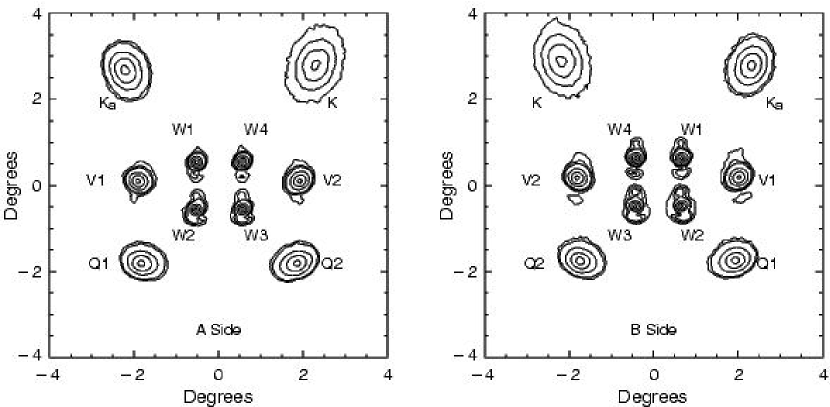
Figure 1: Jupiter maps of the A and B side focal planes (Bennett et al., 2003c) in the reference frame of the observatory. The contour levels are at 0.9, 0.6, 0.3, 0.09, 0.06, 0.03 of the peak value. W1 and W4 are the “upper” W-band radiometers. In W band, the lobes at the 0.09 contour level ($\approx-10~{}$dB) and lower are due to surface deformations.

Figure 1 shows the “raw” beams from both telescopes. A number of features are immediately evident. As expected, all beams are asymmetric and the V and W band beams have significant substructure at the $-10$ to $-20$ dB level. The asymmetry results because the feeds (Barnes et al., 2002) are far from the primary focus. The substructure arises because the primary mirror distorts upon cooling with an rms deviation of $\sigma_{z}=0.024~{}$cm and correlation length of $l_{c}\approx 10~{}$cm (Page et al., 2003).

The Jupiter data are analyzed both as maps binned with $2.4^{\prime}\times 2.4^{\prime}$ pixels and as time ordered data (TOD). These data products are analyzed separately. In addition, full flight simulations are used to test the software.

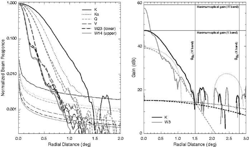
Figure 2: Left: The symmetrized beams (normalized at unity) and noise levels (below) from two seasons of Jupiter observations. Both polarizations have been combined. The noise rises at small radii because there are fewer pixels over which to average. With four years of observations, the noise level will be reduced by a factor of two. Right: The K (black) and W3 (grey) symmetrized beam profiles with their associated Ruze patterns (§2.1). The noise level is at 20 dBi in all bands as seen in the plot (missing data corresponds to negative values). The maximum optical gains are 47.1 and 59.3 dBi in K and W bands as indicated by the horizontal lines. Table 1 shows the gain budget. The dashed lines are the Ruze patterns assuming a Gaussian shaped distortion with the parameters in the text. The lighter shaded dotted lines that meet the dashed lines at $\theta=0$ are for a tophat shaped distortion. In W band, the tophat prediction, which has a prominent lobe at $\theta=2\fdg 5$ clearly does not fit the data. Plots for W14 show the Ruze pattern to be above the beam profile for $\theta<1^{\circ}$ suggesting the magnitude of the deformations is not greater than those we use. However, some fraction of $\Omega_{B}$ could be at or near the noise level for $1\fdg 5<\theta<2\fdg 0$. The vertical straight lines indicate the cutoff radii, $\theta_{Rc}$, for the Gaussian distortion model.

Figure 2 shows the beams in profile after symmetrization. In the Jupiter map analysis, the symmetrization procedure consists of smoothly interpolating the beam to $0.015^{\prime}\times 0.015^{\prime}$ pixels with a 2-D spline and then azimuthally averaging in rings of width $1.2^{\prime}$. Due to noise, the maximum value in a map is often not on the best symmetry axis, though it is generally within one pixel of it. The symmetrized beam has the same solid angle as the raw beam to within $0.3$%. The normalized symmetrized beam is called $b^{S}$. In the TOD analysis, the data are fit to a series of Hermite functions (§3) according to their angular separation from a predetermined centroid. The best centroid is determined iteratively. The analysis includes the effects of the sampling integration and pre-whitening procedure (Hinshaw et al., 2003) but does not have the intermediate step of mapmaking and thus is independent of the $2.4^{\prime}$ pixelization. There are low signal to noise modes in the Jupiter maps that do not affect the window functions and to which the Hermite method is insensitive. Generally, the Hermite beams are used for $\ell$-space quantities, such as the window function, and the Jupiter maps are used for real space calculations.

2.1 Beam solid angles and uncertainties

Linking the calibration of observations of the CMB at $\ell=1$ to compact sources at $\ell\approx 1000$ requires knowledge of the beam profile over a large range of angular scales. The width in $\ell$-space can be characterized by the total beam solid angle, $\Omega_{A}=\int b_{T}\,d\,\Omega$, where $b_{T}$ is the full sky beam profile normalized to unity on the boresight. In our analysis, the beam is divided into two parts: $\Omega_{A}=\Omega_{B}+\Omega_{S}$ where $\Omega_{B}$ is the main beam solid angle and $\Omega_{S}$ is the portion associated with the sidelobes. Ideally $\Omega_{S}=0$ but this is not an appropriate approximation for WMAP, especially in K band. Generally, $\Omega_{B}$ is found by normalizing a map to the best fit peak value, and then integrating out to some radius. For WMAP, $\Omega_{B}$ does not reach a stable value as the integration radius is increased because of the imperfect knowledge of the background. This may be seen with the following estimate. The net statistical uncertainty in the WMAP data in a patch of radius $3\deg$ is $\approx 6~{}\mu$K (the noise is $\approx 0.85$ mK in each $2.4^{\prime}\times 2.4^{\prime}$ pixel). If the background could be removed to this level, the resulting solid angle temperature product would be $T\Omega=5\times 10^{-2}~{}\mu$K sr. By comparison, $T_{J}^{m}\Omega_{B}\approx 4~{}\mu$K sr in W-band ($T_{J}^{m}\approx 200~{}$mK and $\Omega_{B}\approx 2\times 10^{-5}~{}$sr ). Given that both the region near Jupiter and the region being compared to must be known to this level and that $T\Omega$ grows with radius, deviations of a few percent are not unexpected. As the signal to noise improves throughout the mission, this limitation will be alleviated.

In order to derive a consistent set of solid angles, we define a cutoff radius, $\theta_{Rc}$, out to which the solid angle integration is performed. As shown in Page et al. (2003), the global properties of the beam may be modeled by a core plus a “Ruze pattern” (Ruze, 1966) that is a function of the surface correlation length and rms roughness. We assume that $l_{c}$ is unchanged from the pre-launch measurements at 70 K. (The in-flight temperatures of the primaries are 73 K and 68 K for the central and top thermometers for both A and B sides.) Table 2 shows how the main beam forward gain, $4\pi/\Omega_{B}$, is reduced by the sampling and surface deformations. The agreement between the measurements and the expectations is evidence that the main beam effects have been accounted for and that the in-flight $\sigma_{z}$ is consistent with the ground-based measurement. Physical models of the optics, in §2.5, give further evidence for this.

We define $\theta_{Rc}$ as the radius that contains at least 99.8% of the modeled main beam solid angle. These values are 2$\fdg$8, 2$\fdg$5, 2$\fdg$2, 1$\fdg$8, 1$\fdg$5 respectively for K through W bands and agree with values derived from the physical model of the optics. Figure 2 shows examples of the K- and W-band beams and their Ruze patterns. The solid angles resulting from the integrals over the Jupiter maps with a cutoff radius of $\theta_{Rc}$ are given in Table 3.

The uncertainty in the main beam solid angle primarily affects the determination of the flux from point sources and spatially localized features in real space. Solid angle uncertainties affect the angular spectrum through the width of the $\ell$-space passband as discussed in §3. The uncertainty is assessed three ways:

1. The solid angles are determined from simulations that have been processed in the same way the flight data are computed. The rms deviation between the input and recovered solid angle for 20 measurements (10 on the A side and 10 on the B side) is 1.1%. The formal statistical uncertainty is between 0.7% and 1% depending on band.

2. The scatter in the derived temperature of Jupiter is found for all detector/reflector combinations. Each feed is mapped in two polarizations by two detectors during two seasons for a total of eight measurements. The statistical uncertainty of the mean of the eight measurements is 2.6% in K band and $\approx 1.1$% in Ka through W bands. The K beam result has a relatively low amplitude, $\approx 13.5$ mK, and is wide, making it difficult to measure. It is also the most susceptible to the effective frequency and to incompletely subtracted Galactic contamination.

   The systematic uncertainty is also determined from the Jupiter maps. The uncertainty on Jupiter’s measured amplitude is $\approx 0.5$% and is always subdominant to the uncertainty in the solid angle. We assume that Jupiter’s temperature is the same for all measurements within a band. (The intraband effective frequencies are close enough to be insensitive to Jupiter’s spectrum.) The uncertainty of $\Omega_{B}$ is increased until $\chi^{2}/\nu=1$ for fits to Jupiter’s temperature within a band. This results in uncertainties of 2.6%, 1.2%, 1.2%, 1.1%, & 2.1% per DA per side for K through W bands.

3. The solid angles are recomputed by direct integration after increasing $\theta_{Rc}$ to 3$\fdg$7, 3$\fdg$3, 2$\fdg$9, 2$\fdg$4, 2$\fdg$0 respectively for K through W bands. For the 10 DAs on both A and B sides, the rms deviation between the original $\theta<\theta_{R_{c}}$ and recomputed solid angles is 0.8% with no clear trend in the sign of the deviation except in W-band. In W-band, the solid angles with the increased $\theta_{Rc}$ are systematically larger by 0.8% on average, suggesting a potential bias. The most likely explanation is that the shape of the surface distortions is not Gaussian as assumed for the Ruze model. From Figure 2, one sees that the level of the potential contribution is at $\approx-35$ dB, just beyond $\theta_{Rc}$. We term this region the beam pedestal. To account for the bias, the W-band solid angles are increased by 0.8% over the nominally computed value and assigned an additional uncertainty of 0.4%, added in quadrature. The net uncertainty is still 2.1%. This increase is accounted for in Table 1 and discussed in the context of the window functions in §3.2. For the year-one data release, we treat this as a systematic deviation from our model and account for it in the analysis. Future analyses, with more data, will treat this effect with a more comprehensive beam model (§2.5) and will determine the source of the pedestal in the beam.

The uncertainties in the solid angles used throughout the analysis encompass the systematic effects in items 2 and 3. These uncertainties should be interpreted as “1$\sigma$.”

2.2 Sidelobes

The distinction between the main beams and the sidelobes is at some level an arbitrary definition. The structure that holds the feed horns scatters radiation into a large region around the main beams. In other words, the main beam does not contain the total solid angle of the full sky beam (Table 7, Page et al. (2003)). The fraction of the total solid angle outside $\theta_{Rc}$ is 0.037, 0.012, 0.012, 0.0022, and 0.001-0.003 in K through W bands respectively. For example, in K band, the region with $\theta<\theta_{Rc}$ contains 99.8% of the modeled main beam solid angle ($\Omega_{B}$) but only 96.4% of the total solid angle ($\Omega_{A}$).

The sidelobes have two effects on the interpretation of the data. The first arises from Galactic contamination. As shown in Barnes et al. (2003), the sidelobe leakage affects primarily $\ell<20$ and is not significant for Ka, Q, V, and W bands. The second arises from the sidelobe contribution to the calibration of features at $\ell>20$. For example, point sources are detected only in the main beam and the measured temperature profile of a point source corresponds to only a main beam calibration. The dipole, however, is a full beam calibrator. Thus, to obtain the true flux of a point source, to a good approximation one multiplies the flux as calibrated by the dipole by 1.037, 1.012, 1.012, 1.002, and 1.003 in K through W bands respectively.

For the year-one release, only the K-band map is corrected for the Galactic sidelobe contribution. However, all the point source fluxes in Bennett et al. (2003a) and Jupiter fluxes given below have been corrected in all bands. The uncertainty of the correction is taken as half the correction factor, or 2%, 0.5%, 0.5%, 0.1%, and 0.2% in K through W bands respectively.

2.3 Effective Frequencies

Because of WMAP’s broad frequency bandwidth, sources with different spectra have different effective frequencies. The effective frequency for a source that is small compared to the beam width (Page et al., 2003) is:

$$\nu_{e}\equiv{\int\nu f(\nu)G_{m}(\nu)\nu^{-2}\sigma(\nu)d\nu\over\int f(\nu)G_{m}(\nu)\nu^{-2}\sigma(\nu)d\nu}$$ (2)

where $f(\nu)$ is the measured radio frequency (RF) passband and $G_{m}(\nu)$ is the maximum (forward) gain. The spectral dependence of the source is $\sigma(\nu)\propto\nu^{\alpha}$ with $\alpha$ the spectral index ( $\alpha\approx-0.7$ for synchrotron, $\alpha\approx-0.1$ for free-free, $\alpha=2$ for Rayleigh-Jeans, and $\alpha\approx 4$ for dust) or $\sigma(\nu)\propto\nu^{4}\exp(h\nu/k_{B}T_{CMB})/(\exp(h\nu/k_{B}T_{CMB})-1)^{2}$ for the CMB. (The variation of loss across the band is negligible.) For full beam sources, such as the CMB or the calibrators used in ground testing, the small dependence on the forward gain should not be included and the central frequencies in Jarosik et al. (2003a) should be used. At high $\ell$ or for point sources, the effective center frequency, and therefore the thermodynamic to Rayleigh-Jeans correction, changes. The magnitude and sign of the change depend on the relative weights of the radiometer passbands and forward gain. This small effect ($<0.2~{}$GHz or $<0.1$%) in the conversion was not included in the year-one maps.

The passbands for the two polarizations in a DA differ slightly (Jarosik et al., 2003a). Thus, the two polarizations for one telescope (e.g., A side) have different passbands. On the other hand, the optical gain as a function of frequency is the same for both polarizations of one telescope but differs between the A and B sides. In Table 3, for the CMB, we give the effective frequencies from equation 2 for the average of the two RF passbands for the A and B sides separately. We also give the effective frequencies for both polarizations separately (Table 11, Jarosik et al. (2003a) ) for a source that fills the beam. The table shows that the effect of the optics on the passbands is small.

2.4 Temperature of Jupiter

The observations of Jupiter and the CMB dipole with WMAP result in a calibration of Jupiter calibrated with respect to the CMB dipole. After coadding the data over polarization and season, a fit is made to Jupiter’s temperature. Before the fit is done, a correction is applied. The loss in the input optics on the A and B sides differs by $\approx~{}1$% (Table 3, Jarosik et al. (2003a)). Therefore, Jupiter and the CMB do not have the same apparent temperature when measured through the A and B telescopes. The signature of the effect is that the average of the A-side temperature data is offset from that of the B-side data. This effect is accounted for in the year-one sky maps but not in the Jupiter maps. After the A/B imbalance, sidelobe corrections, and the W-band pedestal correction, all measurements of $T_{J}$ in one microwave band are fit to a single temperature. We find that $T_{J}$, in brightness temperature, is given by $134\pm 4$, $146.6\pm 2.0$, $154.7\pm 1.7$, $163.8\pm 1.5$, $171.8\pm 1.7~{}$K in K through W bands respectively. The uncertainty is dominated by the uncertainty in the solid angles, in the sidelobe corrections, and in the 0.5% intrinsic calibration uncertainty (Hinshaw et al., 2003). These values are the temperature one would measure by comparing the flux from Jupiter to that from blank sky. To obtain the absolute brightness temperature, one must add to these the brightness temperature of the CMB (2.2 K, 2.0 K, 1.9 K, 1.5 K, and 1.1 K in K through W bands, respectively). A future paper will compare this result to other measurements and assess the stability and polarization characteristics more completely.

2.5 Physical Model of Beams

The dominant surface deformation that leads to the distortions of the main beams comes from the “H-shaped” backing structure that holds the primary mirrors. A simple Fourier transform of the aperture with an additive H-shaped distortion reproduces many of the features in Figure 1, but photogramatic pictures (Page et al., 2003) of the cold surface indicate that the surface structure is more complicated. For the purposes of the year-one analysis, the Gaussian distortion model is sufficient, but for future analyses a more accurate model is desired.

The full beam is modeled using a physical optics code (DADRA, Rahmat-Samii et al. (1995)) that predicts the beam profile given the detailed physical shape of the optics. The primary surface deformation is parametrized with a set of Fourier modes the amplitudes of which are the fit coefficients. (In the pre-launch cryogenic tests, there was no evidence for a significant change in shape of the secondary.) A minimization loop finds the surface shape parameters that simultaneously fit the two V-band and four W-band beam maps of Jupiter.

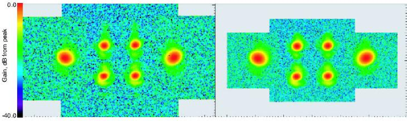
Figure 3: Left: A mosaic of the A-side W and V-band measured beams. One should focus on the main beams areas. Different noise levels in the constituent mosaics lead to apparent artifacts away from the beam centers. Right: Model of the A-side beams based on the physical optics calculations described in the text. The same surface is used for all beams. Most of the features in the measured beams are reproduced in the model indicating that the source of the distortions has been identified. The noise from the measurement has been added to model on the right to make the comparison more direct. The separation between different W-band beams is $1\fdg 1$, less than the cutoff radius for the determining the W-band solid angles.

The program is computationally intensive because the full physical optics calculation for all beams is recomputed for each iteration. A qualitative comparison of the measured and modeled beam patterns is shown in Figure 3 from which it is clear that the amplitude and phase of much of the surface deformation has been identified. The program has not run long enough to converge in all bands, so it is not yet used in the beam analysis. At this stage, though, the model gives us confidence that we are not missing significant components of $\Omega_{B}$ and that our interpretation of the beams is correct.

2.6 Temperature Stability and Reflector Emissivity

The WMAP orbit in the L₂ environment results in extremely good thermal stability. The instrument has an array of thermometers on the optical components with sub-millikelvin resolution (Jarosik et al., 2003b). By binning the temperature data synchronously with the spin rate and the position of the Sun, we detect a synchronous thermal variation in the optics. The top and middle of the primary have a peak-to-peak amplitude of $\approx 0.23$ mK. We believe this is due to scattering of solar radiation off the rim of the solar array. The tips of the secondary mirrors show a maximal variation of 0.04 mK peak-to-peak, with the rest of the secondaries much less. There is no evidence for any thermal variation due to illumination by the Earth or Moon. The 0.23 mK is well below the conservative bound of 1.5 mK in Page et al. (2003) and below the 0.5 mK rms requirement in the systematic error budget.

We bound the emissivity, $\epsilon$, of the reflectors using a similar method. After subtracting the CMB dipole from the TOD, the radiometric signal is coadded in Sun-synchronous coordinates following the method outlined in Jarosik et al. (2003b). The net spin synchronous radiometric signal detected is 0.4 $\mu$K peak-to-peak (0.014 $\mu$K rms) in the combined W and V bands. Therefore, an upper bound on the emissivity of the surface is 0.002. The predicted emissivity is $0.0005$.

2.7 Polarization from Optics

Each DA measures two orthogonal differential polarizations from each pair of feeds (e.g., K11A and K11B form one difference and K12A and K12B form the other difference). The Stokes Q and U components are found by differencing these two signals in the time stream, determining the components relative to a fixed direction on the sky, and then producing a map with the mapmaking algorithm (Kogut et al., 2003; Hinshaw et al., 2003). WMAP was designed to have cross-polar leakage of $<-22$ dB in all bands (Page et al., 2003) to enable a measurement of the polarization of the CMB. This specification was met and demonstrated in pre-launch ground tests with a polarized source.

To assess the degree of the similarity of the two polarization channels, we take the A-side beam maps for both polarizations from one feed (e.g., KA11 (’P1’) and KA12 (’P2’)), difference them, integrate over the difference map, and then divide by $T\Omega$ from Jupiter. The resulting fractional signal for the A side is 8.1%, 2.5%, 0.2%, 0.4%, -2.8%, -2.7%, 0.3%, 0.5%, 1.6%, and 0.9% in K1 through W4 bands. For the B side it is 6.5%, -0.1%, -3.3%, 4.0%, 0.4%, 1.0%, -0.5%, -0.1%, 2.7%, -0.5%. The statistical uncertainty for the difference in polarizations is $\approx 1.2$% and the measured rms of all Ka through W values is 1.8%. For a polarized source, the sign of the difference changes when P1-P2 is determined on the A and B sides.

The difference between the beams (P1-P2) from the Jupiter maps is larger than expected but there are no clear trends in Ka through W bands and no clear detections of polarization. For K band, there is a clear excess at a level larger than can be attributed to the optics. As Jupiter is nearly a thermal source, the difference is not due to a frequency mismatch (Kogut et al., 2003) between the dipole and Jupiter. However, the difference in effective frequencies of 1.0 GHz (P1 and P2, Table 3) leads to a difference in solid angle of order 10% (Table 5, Page et al. (2003)), enough to explain the effect. The net effect is smaller in the higher frequency bands because of the low edge taper. For the year-one analysis, the slight difference in the effective frequency for the bands is not corrected. Instead, the uncertainty is absorbed in the uncertainty of the average solid angle.

The CMB is polarized at the $\approx 5$% level, in temperature units, and the temperature-polarization correlation is at the $\approx 15$% level. The CMB polarization signal comes from scales larger than the size of the beam and so no particular band mismatch affects the CMB polarization results. In addition, the CMB signal is derived from the sum over multiple bands.

3 Calculation of window functions

The characteristics of the CMB are most frequently expressed as an angular spectrum of the form $l(l+1)C_{l}/2\pi$ (Bond, 1996) where $C_{l}$ is the angular power spectrum of the temperature:

$$T({\bf n})=\sum_{\ell,m}a_{\ell m}Y_{\ell m}({\bf n}),~{}~{}~{}\langle a^{*}_{\ell^{\prime}m^{\prime}}a_{\ell m}\rangle=\delta_{\ell^{\prime}\ell}\delta_{m^{\prime}m}C_{\ell}$$ (3)

where n is a unit vector on the sphere and $Y_{\ell m}$ is a spherical harmonic.

The beam acts as a spatial low-pass filter on the angular variations in $T({\bf n})$ such that the variance of a noiseless set of temperature measurements is given by

$$C(0)\approx\sum_{\ell}{(2\ell+1)C_{\ell}\over 4\pi}w_{\ell}$$ (4)

where $w_{\ell}$ is the window function which encodes the beam smoothing. It is normalized to unity at $\ell=0$ as discussed below.

The window functions are expressed following the conventions of White & Srednicki (1995). The window function depends on the mapping function $M({\bf n},{\bf n}^{\prime})$ which describes how the experiment convolves the true sky temperature $T({\bf n}^{\prime})$ into the observed temperature ${\widetilde{T}}({\bf n})$,

$${\widetilde{T}}({\bf n})=\int d\Omega_{{\bf n}^{\prime}}M({\bf n},{\bf n}^{\prime})T({\bf n}^{\prime}).$$ (5)

For WMAP, $M({\bf n},{\bf n}^{\prime})$ for one feed is a weighted average of the beam response $B({\bf n},{\bf n}^{\prime})$ that accounts for the smearing due to the finite arc scanned over an integration period and the azimuthal coverage of the observations in each pixel. The symmetrized beam, $B^{S}$, is an excellent approximation to the mapping function.

The full window function is given by:

$$w_{\ell}({\bf n}_{1},{\bf n}_{2}) \equiv \int d\Omega_{{\bf n}^{\prime}_{1}}\int d\Omega_{{\bf n}^{\prime}_{2}}M({\bf n}_{1},{\bf n}^{\prime}_{1})M({\bf n}_{2},{\bf n}^{\prime}_{2})P_{\ell}({\bf n}_{1}^{\prime}\cdot{\bf n}_{2}^{\prime})$$ (6)

$$= {4\pi\over(2\ell+1)}\sum_{m=-\ell}^{+\ell}\int d\Omega_{{\bf n}^{\prime}_{1}}\int d\Omega_{{\bf n}^{\prime}_{2}}\,M({\bf n}_{1},{\bf n}^{\prime}_{1})\times$$

$$\,M({\bf n}_{2},{\bf n}^{\prime}_{2})\,Y^{*}_{\ell m}({\bf n}_{1}^{\prime})\,Y_{\ell m}({\bf n}_{2}^{\prime})$$

where $P_{\ell}$ is a Legendre polynomial. The primary quantity of interest is the window function at zero lag, $w_{\ell}({\bf n},{\bf n})$. In this case the total variance of the data, $C(0)$, is the sum of the power in each spherical harmonic weighted by the window. This is directly analogous to low-pass filtering. If the mapping function is independent of celestial position, then

$$w_{\ell} = {4\pi\over(2\ell+1)}\sum_{m=-\ell}^{+\ell}\left|\int d\Omega_{{\bf n}}\,M({\bf n},{\bf n})\,Y^{*}_{\ell m}({\bf n})\right|^{2}$$ (7)

$$= {4\pi\over(2\ell+1)}\sum_{m=-\ell}^{+\ell}\left|m_{\ell m}\right|^{2}$$ (8)

where the $m_{\ell m}$ are the harmonic coefficients of the mapping function.

If the beam is azimuthally symmetric, a further simplification can be made: $\sum_{m=-\ell}^{+\ell}\left|m_{\ell m}\right|^{2}=(2\ell+1)b_{l}^{2}/4\pi$ where $b_{\ell}$ is given by the Legendre transform of the beam

$$b_{\ell}=2\pi\int b^{S}(\theta)P_{\ell}(\cos\theta)d(\cos\theta)/\Omega_{B}.$$ (9)

Thus $w_{\ell}=b_{\ell}^{2}$. For symmetric beams, $\theta$ is used instead of ${\rm acos}({\bf n}\cdot{\bf n^{\prime}})$. For a symmetric Gaussian of width $\sigma_{b}$, we find

$$B_{\ell} \approx 2\pi\sigma_{b}^{2}e^{-\ell(\ell+1)\sigma_{b}^{2}/2}$$ (10)

$$= \Omega_{B}e^{-\ell(\ell+1)\sigma_{b}^{2}/2}$$ (11)

where $B_{\ell}$ is the Legendre transform with units of sr. Because the instrument is calibrated with a dipole signal, the $B_{\ell}$ should be normalized at $\ell=1$. In practice, this is indistinguishable from normalizing at $\ell=0$. Thus, $b_{\ell}=B_{\ell}/B_{\ell=0}=B_{\ell}/\Omega_{B}$ and is dimensionless.

Although WMAP is intrinsically differential, there is essentially no overlap of the beams from opposite sides, so the window functions from each beam may be treated independently and then combined in the end. Thus, the window function for the differential signal is derived from the weighted symmetrized beam

$$b^{S}(\theta)={\Omega^{S}\over 2}\biggl{(}{(1-\overline{x}_{im})|b^{S,A}|\over\Omega^{A}_{B}}+{(1+\overline{x}_{im})|b^{S,B}|\over\Omega^{B}_{B}}\biggr{)}$$ (12)

where $\Omega^{A}_{B}$ and $\Omega^{B}_{B}$ are the main beam solid angles for the A and B side beams, $\Omega^{S}$ is the effective solid angle of the combined beam, and $\overline{x}_{im}$ is $\approx 0.01$ and corrects for the A/B imbalance (Jarosik et al., 2003a) . We use the absolute values to indicate that both beams are treated as positive in this equation. As before, the superscript $S$ denotes a symmetrized beam.

3.1 Window Functions and Their Uncertainties.

We compute the window function for the CMB analysis from $b^{S}$ using an expansion of the symmetrized beam in Hermite polynomials. Hermite functions are a natural basis for the beam as they parametrize deviations from Gaussanity. The expansion also naturally gives the covariance matrix for the $B_{\ell}$ as well.

The Hermite expansion is given by

$$b^{S}(\theta)=\exp(-\theta^{2}/2\sigma_{h}^{2})\sum_{i=0}^{m_{h}}a_{2i}H_{2i}(\theta/\sigma_{h})$$ (13)

where $\theta$ is angular distance from the beam center, $\sigma_{h}$ is the Gaussian width of the beam, and $H_{2i}$ is the Hermite polynomial of order $2n$ (Chapter 22, Abramowitz & Stegun (1972) ). The parameters of the expansion are given in Table 4. A fit is made of the TOD to equation 13. From the fit, the $m_{h}$ coefficients $a_{2i}$ and the $m_{h}\times m_{h}$ covariance matrix $C^{aa^{\prime}}$ are found. The expansion coefficients, $a_{2i}$, are normalized to account for the measured temperature of Jupiter and the normalization of $H_{2i}$.

The transfer function is computed separately for each Hermite polynomial following equation 9:

$$B_{\ell i}=2\pi\int\exp(-\theta^{2}/2\sigma_{h}^{2})H_{2i}(\theta/\sigma_{h})P_{\ell}(\cos\theta)d(\cos\theta)$$ (14)

so that the full transfer function is

$$B_{\ell}=\sum_{i=0}^{m_{h}}a_{2i}B_{\ell i}.$$ (15)

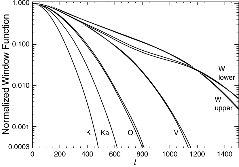
Figure 4: The ten window functions, $w_{\ell}$, computed from the Hermite expansion. The window functions for the two polarizations in each feed are nearly indistinguishable at the resolution of the plot.

The window functions based on equation 15 are shown in Figure 4. From equation 15, one can determine the covariance matrix between $B_{\ell}$ and $B_{\ell}^{\prime}$ as:

$$\Sigma_{\ell\ell^{\prime}}^{B}=\sum_{i,j=0}^{m_{h}}{\partial B_{\ell}\over\partial a_{2i}}C^{aa^{\prime}}_{ij}{\partial B_{\ell^{\prime}}\over\partial a_{2j}}=\sum_{i,j=0}^{m_{h}}B_{\ell i}C^{aa^{\prime}}_{ij}B_{\ell^{\prime}j}.$$ (16)

This matrix has units of sr², is independent of Jupiter’s temperature, and is largest in magnitude at low $\ell$.

Because of the dipole calibration, there is effectively only calibration uncertainty at $\ell=1$. This is accommodated in the formalism by normalizing the beam covariance matrix at $\ell=0$, $b_{\ell}=B_{\ell}/B_{0}$, as shown in Appendix A. We find

$$\Sigma_{\ell\ell^{\prime}}^{b} = \sum_{i,j=0}^{m_{h}}{\partial b_{\ell}\over\partial a_{2i}}C^{aa^{\prime}}_{ij}{\partial b_{\ell^{\prime}}\over\partial a_{2j}}$$ (17)

$$= {1\over{(\Omega^{S})^{2}}}\left(\Sigma_{\ell\ell^{\prime}}^{B}+b_{\ell}b_{\ell^{\prime}}\Sigma_{00}^{B}-b_{\ell}\Sigma_{0\ell^{\prime}}^{B}-b_{\ell^{\prime}}\Sigma_{\ell 0}^{B}\right).$$ (18)

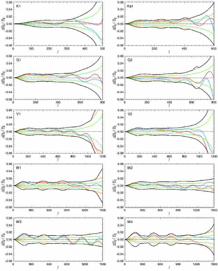
Figure 5: The transfer functions and their statistical and systematic uncertainty. The y axis of each panel shows the fractional uncertainty. The green curve is the statistical uncertainty in the Hermite-based transfer function. The orange curve corresponds to twice the statistical uncertainty (it is mostly hidden by the black curve). The red curve is the fractional difference between the $b_{l}$ computed from the spherical harmonic decomposition of the time stream and the Hermite fit. The blue line is the fractional difference between the $b_{l}$ derived from the Juipter maps, after dividing by the $2.4^{\prime}$ pixelization window function, and the Hermite-based transfer function. The black curve is the adopted 1$\sigma$ uncertainty used in all analyses. It corresponds to the absolute value of the maximum deviation from zero of the red, blue, and orange curves. The uncertainties on the window function, $w_{\ell}$, are twice these, but average down when multiple channels are combined. The uncertainty at $\ell=1$ is small because we calibrate on the CMB dipole. The uncertainty in $\Omega_{B}$ is manifest at high $\ell$.

Equation 18 gives the formal statistical uncertainty in the transfer functions which is shown in Figure 5 for the ten DAs.

The solid angle is a scaling factor for the transfer functions, $b_{\ell}$, and does not directly enter into the uncertainty of the window function. However, the noise that leads to the uncertainty in $\Omega_{B}$ also produces the finite $C^{aa^{\prime}}$. In particular, the uncertainty in the $\ell$ cutoff in the transfer function is manifest as the increased uncertainties at large $\ell$ in Figure 5. Because we found that the scatter in $\Omega_{B}$ was larger than that predicted by the noise by a factor of two in W band (§2.1 item 2), the statistical error bars from equation 18 are inflated by a factor of two in all bands to account for current systematic uncertainties intrinsic to the Jupiter data. This is shown in Figure 5.

3.2 Systematic Uncertainty in the Window Functions

The window functions depend on the treatment of the beams, sky coverage, and analysis method at the few percent level. These systematic effects are included in the window function uncertainty.

To determine the effect of incomplete symmetrization, mapping functions $M({\bf n},{\bf n^{\prime}})$ are computed for coverage corresponding to a pixel near the north ecliptic pole, which has the most symmetric coverage, and for a pixel on the ecliptic, which has the least symmetric coverage. For each mapping function, the full window function (equation 8) is computed and compared to $b_{l}^{2}$ computed from equation 15.

Figure 6 shows the departure of the full window function from the symmetrized window function as a function of $\ell$. For all CMB analyses, the symmetric beam assumption is accurate to 1% for all $\ell$ except for $300<\ell<400$ in Q band. In this range, the instrument noise is significantly larger than the beam uncertainty. The uncertainty in the symmetrization is included in the year-one analysis to the extent that it is accounted for in the uncertainties shown in Figure 5.

In addition to the Hermite-based method, The transfer functions are computed from the Jupiter maps ( using equation 9 ) as well as from a direct transform of the binned TOD (using equation 8). These transforms weight the data differently, and less naturally, than do the Hermite expansion and are thus considered as checks. The difference between the transform methods is shown in Figure 5. As the 1 $\sigma$ error at each $\ell$, we adopt the maximum departure from zero of the two alternative transforms or twice the formal uncertainty derived from $C^{aa^{\prime}}$. This error bound is shown as the outer envelope in Figure 5 and is propagated through all other analyses.

In §2.1, it was shown that the choice of $\theta_{Rc}$ leads to a possible systematic bias in the determination of the total beam solid angle in W band. The Jupiter-based window functions were computed with the extended $\theta_{Rc}$ (§2.1, item 3) and were found to differ from the baseline window functions by at most 0.3% for $\ell<\ell^{w=0.1}$. This demonstrates that $\approx 1$% effects in Jupiter maps can be negligible in $\ell$-space.

4 Beam Parameters for Coadded Data Sets

Most analyses are performed on maps that have been coadded by polarization or frequency (Bennett et al., 2003b; Hinshaw et al., 2003). Table 5 gives the effective solid angles, gains and frequencies for two map combinations. The effective solid angle here is computed with equation 12, so it does not include the $2.4^{\prime}$ Jupiter pixelization. These values should be used for data analyses of the sky maps.

The conversion from flux in Janskys ($10^{-26}$ Wm^-2Hz^-1) to antenna temperature depends on the beam. The flux is modeled as $F_{\nu}\propto(\nu/\nu_{e})^{\alpha}$. For a broad band receiver for which the gain is known at all frequencies, the conversion factor is:

$$\Gamma^{bb}={(c^{2}/8\pi k_{B}\nu_{e}^{2})\int f(\nu)G_{m}(\nu)(\nu/\nu_{e})^{\alpha-2}d\nu\over\int f(\nu)d\nu}$$ (19)

where $G_{m}$ is the maximum gain, $f(\nu)$ is the radiometer band pass, and $k_{B}$ is Boltzmann’s constant. The “bb” superscript indicates that this is a broad band quantity computed from a model of the optics.

For WMAP we report an effective conversion factor of $\Gamma=c^{2}/(2k_{B}\Omega^{S}(\nu_{e}^{ff})^{2})$ for sources with $\alpha=-0.1$. Here, $\Omega_{B}$ is computed from the Hermite beam profiles and $\nu_{e}^{ff}$ is the effective frequency for free-free emission. The fractional uncertainty is the same as for $\Omega^{S}$. The factors are tabulated in Table 5.

5 Conclusions

We have presented the characteristics of the beams in both real space and in $\ell$-space and assessed the uncertainties in both domains. In K, Ka, Q, V, and W bands the uncertainties in the beam solid angles are given by 2.6%, 1.2%, 1.2%, 1.1%, and 2.1%. The uncertainties in the window functions are typically 3% at most values of $\ell$. These values include systematic effects.

We have also presented the formalism in which the beam uncertainties are propagated throughout the analysis. The uncertainties which we adopt are conservative though prudent for this stage of the data analysis.

The K-band sidelobe and W-band pedestal corrections are the only beam-related effects that are added in “by hand” and not treated in the formalism. These effects are significant for real space analyses and are currently negligible for the $\ell-$space CMB analyses.

Jupiter is mapped approximately twice per year. With more data and improved modeling, our knowledge of the beams and window functions will improve over the length of the mission.

The Jupiter maps and window functions are available on-line through the LAMBDA web site at http://lambda.gsfc.nasa.gov/.

6 Appendix A

The covariance matrix of the normalized beam is given by

$$\Sigma_{\ell\ell^{\prime}}^{b}=\sum_{i,j=0}^{m_{h}}{\partial b_{\ell}\over\partial a_{2i}}C^{aa^{\prime}}_{ij}{\partial b_{\ell^{\prime}}\over\partial a_{2j}}$$ (20)

where

$$b_{\ell}={B_{\ell}\over B_{0}}={\sum_{k}a_{2k}B_{\ell k}\over\sum_{k}a_{2k}B_{0k}}$$ (21)

and

$${\partial b_{\ell}\over\partial a_{2i}}={B_{i\ell}\over\sum_{k}a_{2k}B_{0k}}-{\sum_{k}a_{2k}B_{\ell k}\over(\sum_{k}a_{2k}B_{0k})^{2}}B_{0i}.$$ (22)

With the real space beam normalized to unity at $\theta=0$, $\sum_{k}a_{2k}B_{0k}=\Omega^{S}$. After plugging equation 20 into equation 22 there are four terms similar in form to

$${\sum_{k}a_{2k}B_{\ell k}\over(\sum_{k}a_{2k}B_{0k})^{2}}B_{0i}C^{aa^{\prime}}_{ij}{\sum_{j}a_{2k}B_{\ell^{\prime}k}\over(\sum_{k}a_{2k}B_{0^{\prime}k})^{2}}B_{0^{\prime}j}={b_{\ell}b_{\ell^{\prime}}\Sigma_{00}\over(\Omega^{S})^{2}}.$$ (23)

After working through the the other terms, we find equation 18.

Table 1: Selected WMAP beam analysis notation

Symbol(s)	Description
$T_{J}^{m}$	Measured amplitude of Jupiter
$T_{J}$	Brightness temperature of Jupiter
$\Omega_{J}^{ref}$	Reference solid angle of Jupiter
$\Omega_{B}$	Generic main beam solid angle
$\Omega_{B}^{A}$ & $\Omega_{B}^{B}$	Main beam solid angle for A and B sides
$\Omega_{S}$	Generic sidelobe solid angle
$\Omega_{A}$	Antenna solid angle, $\Omega_{A}=\Omega_{B}+\Omega_{S}$
$\Omega^{S}$	Effective solid angle of symmetrized A and B beams combined
$b_{T}(\theta)$	Full sky beam profile normalized with $\int bd\Omega=\Omega_{A}$
$b^{S}(\theta)$	Normalized and symmetrized beam profile
$b_{\ell}$	Beam transfer function normalized to unity at $\ell=0$
$\Sigma^{b}_{\ell,\ell^{\prime}}$	Beam covariance matrix for $b_{\ell}$
$B(\theta)$	Beam profile normalized with $\int Bd\Omega=1$
$B_{\ell}$	Beam transfer function of $B(\theta)$
$\Sigma^{B}_{\ell,\ell^{\prime}}$	Beam covariance matrix for $B_{\ell}$
$w_{\ell}$	Window function normalized to unity at $\ell=0$

Note. — Throughout this paper, small letters (e.g., $b,b_{\ell}$) are used to denote dimensionless quantities normalized at $\theta=0$ or $\ell=0$, and capital letters (e.g., $B,B_{\ell}$) are used to denote quantities normalized with $\Omega_{B}$. The term “transfer function” refers to the Hermite or Legendre transform of a beam. The term “window function” is reserved for the square of the transfer function.

Table 2: Main Beam Forward Gain Budget

Gain	K	Ka	Q	V	W1 & W4	W2 & W3
Maximum optical design gain (dBi)	47.1	49.8	51.7	55.5	58.6	59.3
$e^{-k^{2}\sigma_{z}^{2}}$	0.99	0.97	0.95	0.90	0.78	0.78
After scattering (dBi)	47.0	49.7	51.5	55.1	57.5	58.2
After sampling (dBi)	47.0	49.6	51.4	54.9	57.3	57.9
Measured in flight (dBi)	47.3	49.4	51.4	54.6	57.7	57.6

Note. — The forward gain budget for representative beams. The first row gives the as-designed forward gain that would be achieved with a stationary satellite with ideal reflectors. The next line gives the gain reduction factor from the Ruze formula (Ruze (1966), $k$ is the wave vector, $\sigma_{z}$ is given in the text). The scattering reduces the gain to the values given in the line labeled “after scattering.” The finite integration time for each data sample results in a slight smearing of the beam, reducing it to the values in the line labeled “after sampling.” For reference, 1% corresponds to 0.043 dB.

Table 3: Main Beam Solid Angles, Gains, & Effective Frequencies

Beam	$\Omega_{B}$	$G_{m}$	$\nu_{e}^{sync}$	$\nu_{e}^{ff}$	$\nu_{e}^{cmb}$	$P1\nu_{e}^{cmb}$	$P2\nu_{e}^{cmb}$	$\nu_{e}^{RJ}$	$\nu_{e}^{dust}$
	(sr)	(dBi)	(GHz)	(GHz)	(GHz)	(GHz)	(GHz)	(GHz)	(GHz)
K1A	$2.44\times 10^{-4}$	47.1	22.42	22.50	22.76	22.36	23.18	22.77	22.95
K1B	$2.36\times 10^{-4}$	47.3	22.47	22.55	22.80			22.80	22.98
Ka1A	$1.43\times 10^{-4}$	49.4	32.67	32.74	32.98	32.84	33.19	32.99	33.17
Ka1B	$1.45\times 10^{-4}$	49.4	32.61	32.68	32.92			32.93	33.10
Q1A	$0.869\times 10^{-4}$	51.6	40.54	40.64	40.97	40.96	40.79	40.88	41.18
Q1B	$0.903\times 10^{-4}$	51.4	40.58	40.67	40.94			40.99	41.20
Q2A	$0.911\times 10^{-4}$	51.4	40.48	40.56	40.83	40.84	40.23	40.99	41.03
Q2B	$0.895\times 10^{-4}$	51.5	40.43	40.51	40.79			40.80	40.99
V1A	$0.405\times 10^{-4}$	54.9	60.24	60.40	60.91	59.32	61.22	60.96	61.36
V1B	$0.439\times 10^{-4}$	54.6	60.22	60.38	60.90			60.95	61.35
V2A	$0.426\times 10^{-4}$	54.7	60.95	61.10	61.58	61.72	60.75	61.63	62.00
V2B	$0.421\times 10^{-4}$	54.7	60.93	61.09	61.57			61.62	62.00
W1A	$0.196\times 10^{-4}$	58.0	92.85	93.08	93.72	93.71	93.27	93.89	94.47
W1B	$0.213\times 10^{-4}$	57.7	92.74	92.97	93.61			93.78	94.37
W2A	$0.214\times 10^{-4}$	57.7	93.33	93.50	93.97	93.58	94.35	94.10	94.54
W2B	$0.233\times 10^{-4}$	57.3	93.38	93.55	93.04			94.17	94.61
W3A	$0.205\times 10^{-4}$	57.9	92.42	92.58	92.03	92.44	93.39	93.15	93.57
W3B	$0.235\times 10^{-4}$	57.3	92.45	92.61	93.07			93.19	93.63
W4A	$0.203\times 10^{-4}$	57.9	93.25	93.45	94.01	94.33	93.18	94.17	94.68
W4B	$0.213\times 10^{-4}$	57.7	93.19	93.39	93.96			94.11	94.63

Note. — The $\Omega_{B}$ are derived from the Jupiter maps and include the smearing from the $2.4^{\prime}$ pixelization. These solid angles should be used for working with the Jupiter maps. The forward gain is $G_{m}=4\pi/\Omega_{B}$. The effective frequencies are for sources smaller than the beam size (except for entries P1 and P2). For diffuse sources such as the CMB anisotropy, one should use the tabulation in Jarosik et al. (2003a). The columns with the P1 and P2 labels are for the two polarizations and come directly from Table 11 in Jarosik et al. (2003a). They are the same for the A and B sides. By comparing P1 and P2 with $\nu_{e}^{cmb}$ from the previous column, one can assess the effects of the optical gain on the passband. The $1\sigma$ uncertainty on the effective frequency is $0.1$ GHz though the values are given to 0.01 GHz so the trends may be assessed.

Table 4: Transfer Function and Window Function Parameters

	K	Ka	Q	V	W14	W23
$m_{h}$	10	30	30	50/70	70	70
$\sigma_{h}$ (deg)	0.348	0.268	0.210	0.139	0.089	0.088
$\ell^{w_{\ell}=0.5}$	128	163	200	265	300	260
$\ell^{w_{\ell}=0.1}$	240	320	400	580	840	700

Note. — Parameters used in the beam fits and their assessment. The number of terms in the Hermite expansion is given by $m_{h}$ and the Gaussian width for the expansion are given by $\sigma_{h}$. The $\ell$ value for which the normalized window is 0.5 is $\ell^{w_{\ell}=0.5}$ and similarly for $\ell^{w_{\ell}=0.1}$.

Table 5: Main Beam Solid Angles, Gains, $\Gamma$, and Effective Frequencies for Combined Maps

Beam	$\Omega^{S}$	$\theta_{FWHM}$	$G_{m}$	$\Gamma$	$\nu_{e}^{cmb}$
	(sr)	(deg)	(dBi)	($\mu$K/Jy)	(GHz)
For 10 maps
K	$2.39\times 10^{-4}$	0.82	47.2	268	22.8
Ka	$1.43\times 10^{-4}$	0.62	49.4	213	33.0
Q1	$0.879\times 10^{-4}$	0.48	51.6	224	40.9
Q2	$0.900\times 10^{-4}$	0.48	51.4	220	40.5
V1	$0.418\times 10^{-4}$	0.33	54.8	214	60.3
V2	$0.416\times 10^{-4}$	0.33	54.8	210	61.2
W1	$0.199\times 10^{-4}$	0.21	58.0	190	93.5
W2	$0.215\times 10^{-4}$	0.20	57.7	173	94.0
W3	$0.213\times 10^{-4}$	0.20	57.7	179	92.9
W4	$0.202\times 10^{-4}$	0.21	57.9	185	93.8
For 5 maps
K	$2.39\times 10^{-4}$	0.82	47.2	269	22.8
Ka	$1.43\times 10^{-4}$	0.62	49.4	213	33.0
Q	$0.889\times 10^{-4}$	0.49	51.5	222	40.7
V	$0.417\times 10^{-4}$	0.33	54.8	212	60.8
W	$0.206\times 10^{-4}$	0.21	57.8	182	93.5

Note. — The values for $\nu_{e}^{cmb}$ are the average of the values in one band as given by Jarosik et al. (2003a). They are appropriate for the CMB anisotropy. The top ten entries are for the ten maps in which the two polarizations have been combined. The bottom five are for the maps combined by polarization and band. A useful characteristic beam resolution is the full width at half the beam maximum, $\theta_{FWHM}$, though the beams are not Gaussian. The values for $\Gamma$ are for a source with a free-free spectrum. The K-band value is appropriate for the sidelobe corrected map described in Hinshaw et al. (2003). For year-one analyses using $\Omega^{S}$ and $\Gamma$, we recommend uncertainties of 2.6%, 1.2%, 1.2%, 1.1%, and 2.1% in K through W band respectively.

Figure 6: A comparison of the window function of a fully symmetrized beam (characteristic of pixels near the ecliptic poles), to the window function of a beam with only partial symmetrization (characteristic of pixels near the ecliptic equator). The solid line is for Q band, the dash line is for V band, and the dot-dashed line is for W band. The vertical lines indicate where the window functions drop to 0.1 of their value at $\ell=0$.

References

- Abramowitz & Stegun (1972) Abramowitz, M. & Stegun, I. A., eds. 1972, Handbook of Mathematical Functions (New York, NY: Dover Press)
- Barnes et al. (2002) Barnes, C., et al. 2002, ApJS, 143, 567
- Barnes et al. (2003) Barnes, C. et al. 2003, ApJ, submitted
- Bennett et al. (2003a) Bennett, C. L. et al. 2003a, ApJ, submitted
- Bennett et al. (2003b) Bennett, C. L., et al. 2003b, ApJ, submitted
- Bennett et al. (2003c) —. 2003c, ApJ, 583, 1
- Bolton et al. (2002) Bolton, S. J. et al. 2002, Nature, 415, 987
- Bond (1996) Bond, J. R. 1996, in Cosmology and Large Scale Structure, Les Houches Session LX, ed. R. Schaeffer (London, UK: Elsevier), 496
- Cheng et al. (1994) Cheng, E. S., et al. 1994, ApJ, 422, L37
- Griffin et al. (1986) Griffin, M. J., et al. 1986, Icarus, 65, 244
- Hinshaw et al. (2003) Hinshaw, G. F. et al. 2003, ApJ, submitted
- Jarosik et al. (2003a) Jarosik, N. et al. 2003a, ApJS, 145
- Jarosik et al. (2003b) —. 2003b, ApJ, submitted
- Kogut et al. (2003) Kogut, A. et al. 2003, ApJ, submitted
- Miller et al. (2002) Miller, A. D. et al. 2002, ApJS, 140, 115
- Netterfield et al. (1997) Netterfield, C. B., Devlin, M. J., Jarosik, N., Page, L., & Wollack, E. J. 1997, ApJ, 474, 47
- Page et al. (2003) Page, L. et al. 2003, ApJ, 585, in press
- Rahmat-Samii et al. (1995) Rahmat-Samii, Y., Imbriale, W., & Galindo-Isreal, V. 1995, DADRA, YRS Associates, rahmat@ee.ucla.edu
- Ruze (1966) Ruze, J. 1966, Proc of the IEEE, 54, 633
- Souradeep & Ratra (2001) Souradeep, T. & Ratra, B. 2001, ApJ
- White & Srednicki (1995) White, M. & Srednicki. 1995, ApJ, 443, 6
- Wu et al. (2001) Wu, J. H. P., et al. 2001, ApJS, 132, 1