First Year Wilkinson Microwave Anisotropy Probe (WMAP ) Observations: Galactic Signal Contamination from Sidelobe Pickup

Abstract

Since the Galactic center is $\sim 1000$ times brighter than fluctuations in the Cosmic Microwave Background (CMB), CMB experiments must carefully account for stray Galactic pickup. We present the level of contamination due to sidelobes for the year one CMB maps produced by the WMAP observatory. For each radiometer, full $4\pi$ sr antenna gain patterns are determined from a combination of numerical prediction, ground-based and space-based measurements. These patterns are convolved with the WMAP year one sky maps and observatory scan pattern to generate expected sidelobe signal contamination, for both intensity and polarized microwave sky maps. Outside of the Galactic plane, we find rms values for the expected sidelobe pickup of 15, 2.1, 2.0, 0.3, 0.5 $\mu$K for K, Ka, Q, V, and W-bands respectively. Except at K-band, the rms polarized contamination is $\ll 1\hbox{$\mu$K}$. Angular power spectra of the Galactic pickup are presented.

1 Introduction

WMAP consists of dual back-to-back Gregorian telescopes designed to differentially measure fluctuations in the Cosmic Microwave Background (CMB) (Bennett et al., 2003a). WMAP is designed to create maps of the microwave sky in five frequency bands, generically labeled K, Ka, Q, V, and W bands, centered on 23, 33, 41, 61, and 94 GHz respectively. Like all radio telescopes, each WMAP beam has sidelobes, regions of nonzero gain away from the peak line-of-sight direction.

The brightest sidelobes for each WMAP beam correspond to radiation paths which, if started from the feeds, miss a telescope reflector and go to regions of the sky far from the main beam. Figure LABEL:optics shows a rendition of WMAP ’s optical structure. The most important sidelobes result from radiation which, if coming from the sky, spills past the primary reflector, striking the secondary either directly or after bouncing off of one of the two radiator panels. These light paths create angularly broad, smooth swaths of antenna gain 20^∘to 100^∘ from the beam peaks. In addition, multiple reflections between the secondary reflector and the front of the Focal Plane Assembly (FPA) of feed horns contribute to a complicated ‘pedestal’ of gain surrounding each beam peak, $\sim 2$^∘to 15^∘ from the beam peak position. Radiation which follows the intended optical path (primary reflector to secondary to feed horn) is considered part of the main beam, and is considered in a companion paper (Page et al., 2003a).

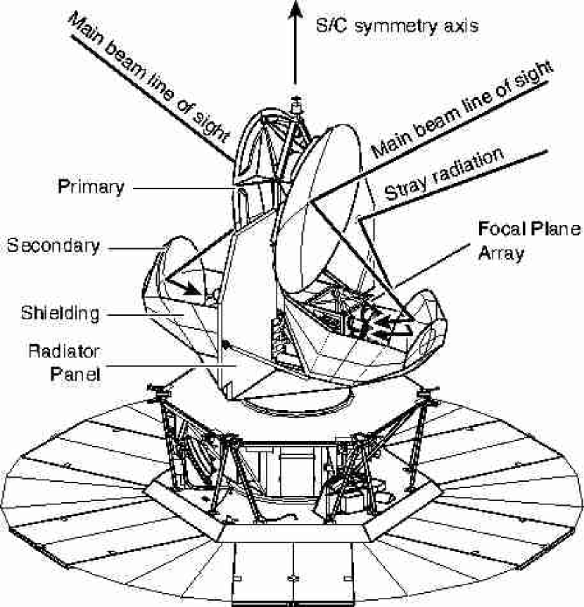
Figure 1: A line drawing of WMAP spacecraft showing the principle optics elements. Radiation from the sky at 68^∘ from the spacecraft axis of symmetry is reflected from the two back-to-back primary reflectors to the two secondary reflectors. Diffraction shields half surround the secondary reflectors to limit radiation from below. The secondaries reflect the radiation into the arrays of feed horns near the center of the instrument. The main diffraction paths are past the edges of the primary reflectors, either directly from the sky or reflecting from the flat radiator panels behind and between the primaries. A higher quality rendering is available on the LAMBDA web site.

Sidelobe gains are most usefully expressed in dBi = $10\log_{10}G(\theta,\phi)$, where the gain $G$ is normalized so that a non-directional antenna has $G(\theta,\phi)=1$, or 0 dBi over $4\pi$ sr. The maximum sidelobe gains range from 5 dBi (in K-band) to 0 dBi (in W-band), from 40 dB to 60 dB below the beam peak gains. For most applications in radio astronomy, such weak responses would be ignorable. However, the relative brightness of Galactic foregrounds makes sidelobe pickup a potentially significant systematic effect for CMB measurements. For the WMAP optics, sidelobe pickup amounts range from $3.7\%$ to $0.5\%$ of total sky sensitivity, K-band to W-band respectively (Page et al., 2003b). Sidelobe pickup introduces a systematic additive signal into the time ordered data (TOD) for each WMAP radiometer differencing assembly (DA). This signal propagates through the map-making algorithm (Hinshaw et al., 2003b) into the final sky map. Since sidelobe pickup does not enter the data stream in the same form as the desired sky signal, the overall contamination in the derived microwave sky maps is a factor of 2 to 3 less than than the sidelobe contribution to the original time ordered data.

For both polarized and unpolarized sky maps, we find that sidelobe contamination is strongest at K-band, growing negligible toward V and W-band. For unpolarized sky maps, the rms sidelobe-induced signal per pixel is $15\ \hbox{$\mu$K}$ at K-band, and $2\ \hbox{$\mu$K}$ or less for Ka, Q, V, and W-bands. The sidelobe-induced polarized contamination is much weaker, $1\ \hbox{$\mu$K}$ rms per pixel at K-band and $\leq 100$ nK in all other bands. (These averages reflect the CMB analysis region of the sky only; specifically the Kp0 cut (Bennett et al., 2003b).) In each case significant sidelobe pickup is confined to the lowest spherical harmonics, $1\leq\ell\mbox{${}_{<}\atop{}^{\sim}$}10$.

This paper is organized as follows. In § 2, we discuss the measurement, physical optics models and calculation of the full sky antenna patterns. In § 3, we describe how these sidelobe patterns are convolved with the one-year measured sky patterns to calculate the Galactic signal contamination within each WMAP first year sky map. Contributions to unpolarized and polarized microwave maps are calculated, and compared with the CMB signal.

A set of sidelobe contamination maps are available with the main WMAP data release.

2 Determination of the Sidelobe Gain Patterns

Antenna gain patterns for WMAP ’s optics were measured at two antenna ranges on the ground, and by using the Moon as a bright source during the spacecraft’s phasing loops (Bennett et al., 2003a). In addition, full-sky antenna patterns were modeled using physical optics software (YRS Rahmat-Samii et al. (1995)). No one measurement or model alone provides enough information to construct an accurate, calibrated, full sky antenna pattern; each has a different region of applicability. In combination, the methods provide a sufficient sidelobe map for the analysis of the WMAP data.

2.1 Ground-based Measurements

Ground-based sidelobe measurements were done at the Goddard Electromagnetic Anechoic Chamber (GEMAC), which used a prototype of one side of the WMAP optics, and an outdoor test range at Princeton University, which used a mockup of the complete spacecraft. Both ranges used only single-frequency (narrow-band) measurements of antenna response. Since both the Galaxy and WMAP radiometers have broadband microwave response, single-frequency gain measurements cannot be taken as the final effective antenna pattern. In both cases, the microwave sources are linearly polarized, permitting polarized measurements of the sidelobe gain patterns.

2.1.1 GEMAC Measurements

The GEMAC is an indoor range consisting of a 3m collimating mirror within an anechoic chamber. The range allows absolute signal calibration to 0.1 dB, with ambient reflection levels ranging from -40 dBi in K-band to -20 dBi in W-band. The collimating mirror renders the incoming wavefronts parallel, placing the source in the telescope’s far-field for all frequency bands. The GEMAC uses an azimuth-over-elevation type mount to rotate the telescope, allowing precise ($0.005\mbox{${}^{\circ}$}$) pointing control. This range cannot observe gains for source elevations lower than $38\mbox{${}^{\circ}$}$ below the spacecraft horizon, or higher than $43\mbox{${}^{\circ}$}$ above it.

Inside the GEMAC range, gain patterns were measured for the optical assembly (feed horns, primary and secondary reflectors, and supporting structure) alone, without radiator panels or solar shields in place. Consequently large sections of the far sidelobes—light which reflects from the radiator panels in flight—wind up in the wrong place. Since the radiator panels are flat reflectors, to an excellent approximation the GEMAC far sidelobe patterns are correct in shape and intensity, though reflected and displaced on the sky.

2.1.2 Princeton Measurements

Princeton’s antenna range has less accurate pointing ($0.1\mbox{${}^{\circ}$}$), and permits only relative signal calibration, but has a significantly lower noise floor than the GEMAC range. At the Princeton test range, the telescope is mounted on a rooftop with an elevation-over-azimuth type drive, while the microwave source is set on a tower 91 m away.

The Princeton range is outdoors, and is arranged so the telescope’s main beam points at empty sky when it is not looking directly at the source. Any reflective pickup must bounce off the ground underneath the telescope, and come in from a disfavored direction. With one exceptional region (described below), the noise floor of the Princeton sidelobe-pattern measurements was determined by receiver noise. Noise floors ranged from -50 dBi in K-band to -35 dBi in Q-band. (V and W-band measurements were limited at the Princeton range by the weakness of the sidelobes, detector noise and uncertainty of calibration.)

At 91 m, the source is in the near field of the telescope’s primary, which has an effective diameter of 1.4 m. Beam peak measurements are out of focus. However, for the purpose of measuring sidelobe response, this condition is immaterial. Sidelobes come from light paths which miss the primary reflector. For this unfocused light, the relevant antenna size is the aperture of the feed horns. As the horn apertures range from 4 to 11 cm in diameter, with the far-field beginning at $4D^{2}/\lambda\sim 4$ m, a source 91 m away is well in the far field. Consequently the Princeton antenna range is usable for measuring antenna patterns everywhere except in the immediate neighborhoods of the beam peaks.

At Princeton, the reflectors were mounted to a complete model of the spacecraft; no important radiation paths should differ materially from the observatory in flight.

In summary the Princeton test range data is usable everywhere away from the main beam peaks, while the GEMAC data is usable everywhere except for reflections and shadows of the satellite radiator panels.

2.2 In-flight Lunar Measurements

The most reliable sidelobe measurements come from the spacecraft’s first orbital phasing loop, just after launch. Data using the Moon as a microwave source were taken between July 2 and July 8 2001. During a total of 4.3 days within this period, WMAP was in normal observing mode, i.e., scanning the sky with a motion incorporating both spin and precession. From the spacecraft point of view, the angular diameter of the Moon varied by a factor of $\sim 2$, with a mean of 1.2^∘. In spacecraft angular coordinates, the Moon swept out a path that provided coverage of the upper hemisphere down to a latitude of 25^∘, which is just above the main beams.

In-flight Moon measurements are preferred to ground measurements because:

The Moon is a roughly thermal microwave source, so Lunar radiation allows broadband measurement of each antenna pattern. We treat the Moon as unpolarized.

The spacecraft/source geometry is exactly as for our CMB measurements. The Moon gives our only direct measurement of the differential sidelobe pickup for the two back-to-back telescopes. All the other measurements are made from a single telescope, half of Figure LABEL:optics.

The radiometers, data collection, and pointing uncertainty on board the observatory are all superior to those on the ground.

The major limitation to using Moon data is the incomplete sky coverage.

2.2.1 Lunar Data Sampling

For each of 10 pairs of feed horns, the sidelobe map comes directly from the time ordered output of the A-B differential radiometer, binned according to the Moon’s position in satellite coordinates. The antenna gain is extracted directly from each measurement:

$$G_{X}({\bf n})={\Delta T^{i,X}_{\rm obs}-\Delta T^{i,X}_{\rm sky}\over T_{\rm Moon}}\left({4\pi{R^{i}_{\rm M-S}}^{2}\over\pi{R_{\rm Moon}}^{2}}\right)\ ,$$ (1)

where ${\bf n}$ is the Moon direction in satellite coordinates, $T_{\rm obs}$ is the observed differential temperature, $R_{\rm M-S}$ is the Moon to satellite distance. The superscripts $X$ and $i$ denote a particular horn position (e.g., Q2) and satellite location/orientation respectively. $\Delta T_{\rm sky}$ is the differential sky signal (CMB + foregrounds) appropriate to the chosen radiometer and observatory orientation. $\Delta T_{\rm sky}$ is calculated from the microwave sky maps. Lastly, $T_{\rm Moon}$ is an effective Lunar temperature for the microwave band in question, and carries the gain calibration uncertainty.

These gain measurements are collected and binned in to HEALPix pixels, creating an unpolarized antenna gain map for each horn pair.

2.3 Physical Optics Modeling

In addition to measurements, antenna gain patterns were modeled for each feed horn position. A physical optics code called Diffraction Analysis of a Dual Reflector Antenna (DADRA), produced by YRS associates (Rahmat-Samii et al., 1995), calculates the full antenna gain and polarization patterns from the profile of a corrugated feed horn, and the precise positions and shapes of the primary and secondary reflectors. Distortions of the reflectors away from their design shapes, measured on the ground, are included in the calculation, as are the radiator panels (modeled as flat, perfect conductors) behind the primary reflector. This calculation is discussed in more detail in (Page et al., 2003b; Barnes et al., 2002).

Physical optics calculations produce absolutely calibrated gains at a single frequency. Near the beam peaks, DADRA-predicted antenna patterns agree within $\sim 3\%$ with gain measurements made in the GEMAC test range.

Further from the main lobe, however, the DADRA predictions of the sidelobe patterns are less accurate. Bright sidelobes are predicted in the right places, with the right shapes, but with lobe gains incorrect by a varying factor of $\sim$ 0.5 to 2, compared to the measurements. As the ratio of predicted to measured gain varies across a single lobe, this is not a calibration issue. We find Princeton, GEMAC and Lunar measured sidelobes in agreement where they overlap, and in disagreement with the physical optics predictions.

The limitation is that DADRA’s physical model of the spacecraft is too simple. The code cannot account for complicated self-reflecting surfaces such as the front of the focal plane assembly. Similarly, the shape of the exposed aluminized Kapton shield around the secondary is complex and not well known. Neither of these surfaces is included in the model. For purposes of working with sidelobe gains, the physical optics results must be considered a reasonable template from an optical system similar to WMAP, rather than a precise model.

Nonetheless, the DADRA predictions prove extremely useful. They yield polarization orientations, difficult to extract from the measurements, and provide evidence of systematic trends in the sidelobes. For example, the far sidelobe intensity in K-band is predicted to vary by a factor of two across the band (from 18–25 GHz, with the longest wavelengths giving the brightest lobes). The DADRA code shows, though, that the sidelobes maintain the same shape as frequency varies: $G(\nu,\theta,\phi)\simeq N(\nu)g(\theta,\phi)$. This is due to the low edge-taper optical design. This relation indicates that single-frequency sidelobe measurements may be used to characterize sidelobes, but their overall calibrations, even when available, may not be assumed correct for calculating Galactic pickup.

Provided the main beams are accurate, this physical optics model may also be used to generate broadband calibrations for the sidelobes. Since

$$\int G(\nu,{\bf n})\,{\rm d}\Omega_{\bf n}=4\pi$$ (2)

for any lossless gain pattern, where $\nu$ is frequency and n is a direction on the sky, then one can write

$$\int G(\nu,{\bf n})f(\nu)\,{\rm d}\Omega_{\bf n}\,{\rm d}\nu=4\pi\int f(\nu)\,{\rm d}\nu\ ,$$ (3)

where $f(\nu)=r(\nu)T_{\rm sky}(\nu)$ carries all source and radiometer frequency dependence. Provided these are known, an accurate physical optics model of the main beam allows for calibration of the total power in the sidelobes:

$$\int_{\rm S}G(\nu,{\bf n})f(\nu)\,{\rm d}\Omega_{\bf n}\,{\rm d}\nu=4\pi\int f(\nu)\,{\rm d}\nu-$$

$$\int_{\rm M}G^{\rm model}(\nu,{\bf n})f(\nu)\,{\rm d}\Omega_{\bf n}\,{\rm d}\nu\ .$$ (4)

Here M and S denote integration over the main beam and sidelobes, respectively. If the main beam gain and source frequency spectrum are known, equation (4) provides a means for calibrating measured sidelobe pickup. The limitations of the physical optics model do not materially affect main beam predictions, and so the right hand side of equation (4) may be used to normalize $G(\nu,{\bf n})$ on the left. This calibration technique has been used for the K through V-band sidelobes. In W-band, direct GEMAC measurements of power outside the main beam disagree with the modeled value, suggesting that our model of the primary reflector does not correctly include its smallest scale distortions.

2.4 Combining Gain Measurements into an Overall Map

To calculate sidelobe-induced Galactic pickup, a full $4\pi$ sr map of antenna gain and polarization is needed for each pair of feed horns. Such a map is most important for the antenna’s highest stray gain regions, all in the satellite’s upper hemisphere. Combined maps are constructed from the measurements and models paying close attention to the weaknesses of each data set, and the self-consistency of assembled whole. Several combined sidelobe antenna patterns are shown in Figure LABEL:sidelobes. The differing angular resolutions and noise levels are attributes of the different data sets. The Lunar data is prominent in the upper third of the spheres. The wide crescents of sensitivity, prominent especially in Q-band, result from radiation spilling past the edge of the primary reflector.

Full sky gain and polarization maps were assembled according to the following rules:

In the immediate neighborhood of the beam peak (within a 10^∘$\times$10^∘square centered on the beam peak), the GEMAC measurements were used. This region includes essentially all light which reflects from the primary reflector. The area is particularly important, since it includes the “beam pedestal,” the area immediately surrounding the main beam, produced by scattering off of the instrument. Outside of the main beam, the pedestal is the highest gain region.

Where available, we use in-flight Lunar data. Lunar measurements are the best available measurements of sidelobe response.

Except at W-band, the overall sidelobe calibration is generated from main beam physical optics predictions, via equation (4). W-band sidelobe maps were calibrated by assuming $T_{\rm Moon}=175$ K, (Bennett et al., 1992). This is lower bound on the brightness for the range of lunar phases observed, and thus the W-band sidelobes are conservative.

Princeton gain measurements are used in regions away from the beam peak, and where Lunar data is unavailable.

Relative calibrations are established by comparing high signal regions where measurements overlap. In K-band, the roughly triangular high response region in Figure 2 finds the Lunar gain measurements are uniformly $60\%$ brighter than what Princeton sees. The Princeton and GEMAC measurements, both measured at single nearby frequencies, are in agreement to within 10%. To generate a consistently calibrated map, GEMAC and Princeton-measured gains were scaled up by $30\%$, Lunar measurements scaled down by $30\%$. This yields a best-guess map for the whole sky with an overall calibration uncertainty of $30\%$. Similar considerations are necessary in each band. As our modeling of the beam and Moon observations mature, this uncertainty will be reduced.

Physical optics predictions are used in any region of the sky not covered by the preceding measurements. Except in V and W bands, DADRA predictions are used exclusively in regions of the spacecraft’s lower hemisphere containing no noticeable features. Where the physical optics predictions are used, their inaccuracy is harmless: in the lower hemisphere the ambient predicted gains range from $-40$ to $-80$ dBi, K to W band. On the observatory, the body of the spacecraft (not present in the optical model) tends to block out light incoming from below the spacecraft horizons, so these gains are systematically high. (The gains are so low that varying them by a factor of 10 or even 100 has no measurable effect on sidelobe pickup.) The important lobes in the upper hemisphere are all at levels of 0 dBi or slightly higher. All measurements made with the source substantially below the satellite horizon are limited by the measurement noise floor. Preflight verification of the solar shield indicated that pickup the Sun’s position is rejected by greater than 90 dB.

Where only single-side measurements are available, the differential gain pattern is constructed by reflection and rotation of the single-side measurements. That is, the differential gain is defined:

$$G_{\rm diff,X}({\bf n}) = G_{\rm A,X}({\bf n})-G_{B,X}({\bf n})$$ (5)

$$= G_{\rm A,X}({\bf n})-G_{A,X}({\bf n}^{\prime})\ ,$$

$$\rm{where}\quad\quad{\bf n}^{\prime}=\left(\begin{array}[]{rrc}1&0&\ 0\\ 0&-1&\ 0\\ 0&0&\ 1\end{array}\right){\bf n}$$

is a reflection in $y$, matching the A-B symmetry of the satellite.

Polarization directions are taken from the polarized optics predictions, except in the immediate neighborhood of the beam peak. In the pedestal region, high signal GEMAC measurements are used. Two measurements of pickup intensity are sufficient to determine the antenna pattern polarization up to a sign ambiguity. This ambiguity is resolved by choosing the polarization direction closest to the one predicted by DADRA.

Physical optics models indicate that the antenna pattern is essentially linearly polarized at every point on the sky. The polarization ellipticity induced by the optics is negligible, both in the main beam and sidelobes. This result is unsurprising; it is inevitable if one family of reflection/diffraction paths to the telescope dominates from each point on the sky. Only separate paths of comparable strength can generate a circularly polarized component to the beam. To an excellent approximation the polarized antenna pattern can be characterized by two fields:

$$G_{X}({\bf n}),\ \mbox{\boldmath$P$}_{X}({\bf n})\ ,$$

where $G$ is the gain, and $P$ is a unit vector everywhere perpendicular to the direction on the sky, ${\bf n}$. $P$ carries an unimportant sign ambiguity and uses three numbers to express a single degree of freedom, but is coordinate independent and simplifies calculation.

Although physical optics predictions get bright sidelobe intensities only roughly correct, the generated polarization directions should be almost exact, within $\sim$ 1^∘. Since all the bright sidelobes come from a single, clear reflection path — e.g., horn to secondary, missing the primary and radiator panels — even geometric optics is sufficient to extract the polarization direction. Differences between the physical optics predictions and the measured antenna gains result from paths that are partially shadowed. This shadowing does not significantly affect the polarization of the remaining light.

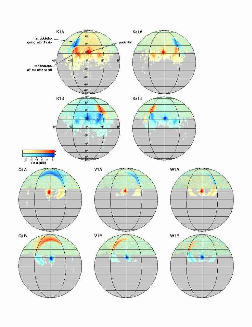
Figure 2: Sidelobe intensity maps for each band. Two hemispheres are shown in spacecraft coordinates for each differential antenna pattern. Positive power (A-side) is shaded pink, negative pickup (B-side) is shaded blue. Gray indicates regions where $|G|<$ -30 dBi. The main beams lie at the center of each pedestal region (middle of the images, at elevations of $\sim 20^{\circ}$). The main beam gain is far off the color scales, at +45 to +60 dBi for K through W bands. The prominent rings of negative gain on the A-side hemispheres come from radiation paths which miss the edge of the B-side primary reflector, and reversely for the B-side image. The V and W band maps were truncated at 10^∘of elevation because the DADRA model is inaccurate below there. A higher quality rendering is available on the LAMBDA web site.

3 Calculating Sidelobe Pickup in Sky Maps

To calculate the sidelobe pickup, the antenna pattern is divided into main beam and sidelobe sections, which are handled separately. We choose to define the main beam to be a circular region centered on the peak gain direction with a cutoff radius, $\theta_{R_{c}}$, determined by Ruze theory predictions of the scattering from the known distortions on the primary (Page et al., 2003a). By band, these radii are K: 2.8^∘, Ka: 2.5^∘, Q: 2.2^∘, V: 1.8^∘, W: 1.5^∘. The response within $\theta_{R_{c}}$ is considered part of the main beam. This response is accounted for in the map-making algorithms and included in the window functions. Everything outside of $\theta_{R_{c}}$ is considered sidelobe gain, treated here as a source of systematic offsets for temperature measurements. The “beam pedestals” are outside of $\theta_{R_{c}}$, and are included in the sidelobes.

When the spacecraft is in an orientation ${\cal O}$ with respect to the Galaxy, where ${\cal O}$ is the rotation matrix from Galactic coordinates into the spacecraft frame, the sidelobe pickup for differencing assembly (DA) $X$ is:

$$\delta T_{X}({\cal O})={1\over 4\pi}\int r_{{}_{X}}(\nu)G_{X}({\cal O}{\bf n},\nu)\biggl{[}T_{\rm sky}({\bf n},\nu)+{}$$

$$T_{\rm pol}({\bf n},\nu)\left\{\mbox{\boldmath$P$}_{\rm sky}({\bf n})\cdot{\cal O}^{\top}\mbox{\boldmath$P$}_{X}({\cal O}{\bf n})\right\}^{2}\biggr{]}\ \,{\rm d}\Omega_{\bf n}\,\,{\rm d}\nu\ .$$ (6)

Here $T_{\rm sky}(\nu)$ is the effective unpolarized sky temperature, $T_{\rm pol},\mbox{\boldmath$P$}_{\rm sky}$ are a temperature and unit vector characterizing the linearly polarized portion of the sky, and $G_{X}$ has been set to zero within $\theta_{R_{c}}$. Here $r_{{}_{X}}(\nu)$ is the radiometer gain, normalized so that $\int\,{\rm d}\nu\,r_{{}_{X}}=1$. For calculations throughout the paper, we will use uncorrected map temperatures $T_{\rm map}$ as an estimate for $T_{\rm sky}$.

In order to calculate $\delta T$ in equation (6), we make the following approximation: Within a band, we integrate out the frequency dependence of the sky,

$$\int{\rm d\nu}\,r_{{}_{X}}(\nu)G_{X}({\bf n},\nu)T_{\rm sky}({\bf n}^{\prime},\nu)={}$$

$$\quad\quad g_{X}({\bf n})T_{\rm sky,\mit X}({\bf n}^{\prime})\ ,\quad\rm and$$ (7)

$$\int{\rm d\nu}\,r_{{}_{X}}(\nu)G_{X}({\bf n},\nu)T_{\rm pol}({\bf n}^{\prime},\nu)={}$$

$$\quad\quad g_{X}({\bf n})T_{\rm pol,\mit X}({\bf n}^{\prime})\ ,$$ (8)

for all directions ${\bf n},{\bf n}^{\prime}$. This is a reasonable approximation, since the microwave sky maps $T_{\rm sky,\mit X}$ were constructed using the same differential radiometers which see the sidelobes. The frequency variation of the sidelobe pattern itself, $G_{X}({\bf n},\nu)\simeq N(\nu)g_{X}({\bf n})$ amounts to an overall calibration uncertainty in the sidelobe strength. This is correct provided that the spectrum of the source of stray light pickup is uniform across the sky. Of course, the various foreground spectra (Bennett et al., 2003c) are manifestly not uniform around the sky as frequency ranges from K to W-bands, 22 to 100 GHz. However, within any particular band (e.g., K band) the brightest foregrounds tend to be dominated by components with similar spectra (e.g., synchrotron radiation.) It is likely that the spectrum of the brightest polarized foregrounds in a band differs from their unpolarized counterparts, so $g_{X}$ may be differently calibrated in equations (7) and (8).

The relevant question for WMAP is: How does the differential sidelobe pickup $\delta T_{X}({\cal O})$ in equation (6) contribute to microwave sky maps? Each measurement in the data stream contributes to its sky map at exactly two pixels: the A and B-side main beam line of sight directions. For a given pixel $p$, the sidelobe contamination may be calculated by taking the appropriate average of $\delta T_{X}({\cal O}_{p})$ for all spacecraft orientations ${\cal O}_{p}$ where the A or B-side beams land on $p$. This average over spacecraft orientations must be weighted according to the flight scan pattern, and should reproduce the result of the full iterative map-making algorithm as closely as possible. Maps of unpolarized and polarized contamination may be generated from the same basic approach.

3.1 Unpolarized Sidelobe Pickup

The radiometer data separates cleanly into polarized and unpolarized components, so the two terms in equation (6) may be handled separately. For unpolarized pickup, ($T_{\rm pol}=0$):

$$\delta T_{X}({\cal O})={1\over 4\pi}\int g_{X}({\cal O}{\bf n})T_{\rm sky,\mit X}({\bf n})\,\,{\rm d}\Omega_{\bf n}\ .$$ (9)

Since the sidelobes are broad and smooth, the integral in equation (9) is calculated accurately using a relatively coarse pixelization of the sphere, HEALPix $N_{\rm side}={}$ 32 or 64. From these varying sidelobe signal in the differential measurements, one can extract the induced systematic contamination of the microwave sky map. We use two techniques to approximate pickup in the final map. Both follow the mapmaking algorithm from the flight data stream.

Applying the first iteration of the mapmaking algorithm (Hinshaw et al., 2003a), one can write:

$$\delta T_{\rm ind\mit,X}({\bf n}) \simeq {1\over 2}\left\langle\delta T_{X}({\cal O})\right\rangle_{{\cal O}:{\cal O}{\bf A}_{X}={\bf n}}$$ (10)

$$-{1\over 2}\left\langle\delta T_{X}({\cal O})\right\rangle_{{\cal O}:{\cal O}{\bf B}_{X}={\bf n}}\ ,$$

where $\left\langle\right\rangle_{\cal O}$ denotes the average over the one-dimensional family of all spacecraft orientations ${\cal O}$ with a main beam pointing at pixel ${\bf n}$. The average $\left\langle\right\rangle_{\cal O}$ is weighted according to the distribution of in-flight spacecraft orientations. For example, pixels near the ecliptic poles are sampled almost evenly among possible spacecraft orientations. For pixels near the ecliptic equator, the flight scan pattern restricts the spacecraft orientation into two disjoint sets, and the full range of orientations is never observed. Similarly, in the full analysis the time ordered data is blanked whenever a main beam crosses a planet, or the reference beam crosses the Galaxy or a bright point source. Spacecraft orientations here are weighted using exactly the same cuts as are used in the full map-making analysis.

Equation (10) yields close to the correct sidelobe contribution, since most of the power in each sky pixel is generated by the first iteration of the mapmaking algorithm (Hinshaw et al., 2003a). However, it is imperfect, since iterations $2$ and higher do have some effect on the data. In particular, the pickup from the bright reference beam pedestal (the B pedestal, if one is averaging over constant A beam peak direction) over-contributes to equation (10). Multiple iterations of the map-making algorithm separate out any power symmetrically localized around the reference pixel, removing most of the reference beam pedestal pickup from the map.

The second method of calculating the map contamination skips the reverse-differencing algorithm altogether. Separating the A and B side pickup according to sign:

$$g_{{}_{A,X}}({\bf n}) = \left\{\begin{array}[]{rcl}g_{X}({\bf n})&:&g_{X}({\bf n})>0\\ 0&:&g_{X}({\bf n})<0\end{array}\right.$$ (13)

$$g_{{}_{B,X}}({\bf n}) = \left\{\begin{array}[]{rcl}0&:&g_{X}({\bf n})>0\\ -g_{X}({\bf n})&:&g_{X}({\bf n})<0\end{array}\right.$$ (16)

one can then write a non-differential mean sidelobe pickup:

$$\delta T_{\rm ind,X}({\bf n})\simeq\hbox{\hskip 72.26999pt}$$

$${1\over 8\pi}\left\langle\int T_{\rm sky,X}({\bf n}^{\prime})g_{{}_{A,X}}({\cal O}{\bf n}^{\prime}){\rm d\Omega_{{\bf n}^{\prime}}}\right\rangle_{{\cal O}:{\cal O}{\bf A}_{X}={\bf n}}+{}$$

$${1\over 8\pi}\left\langle\int T_{\rm sky,X}({\bf n}^{\prime})g_{{}_{B,X}}({\cal O}{\bf n}^{\prime}){\rm d\Omega_{{\bf n}^{\prime}}}\right\rangle_{{\cal O}:{\cal O}{\bf B}_{X}={\bf n}}\ .$$ (17)

No reference beam pedestal ever shows up in equation (17), and so the largest difficulty in the approximation of equation (10) is avoided. This approximation would be exactly right if the instrument yielded the sum of two independent telescope measurements, A and B. If the antenna patterns $g_{{}_{A,X}},g_{{}_{B,X}}$ were symmetric about the A and B side beam peaks, the complete map-making algorithm would give exactly such a sum. The idea of equation (17) is to jump immediately to the end result of map-making.

It is evident from Figure LABEL:sidelobes that the antenna gain patterns are not axially symmetric around their beam peaks. The beam pedestals are somewhat asymmetric, and the far sidelobes show no axial symmetry at all. Since equation (17) removes any regions of negative gain from the beam pattern, cancellations between negative and positive pickup which lower the differential signals do not occur, and the resulting $\delta T$ is biased high. For the same reason, equation (17) is problematic when applied to noisy differential data (the Lunar signal.) Separating differential gain according to sign introduces a bias which again overestimates the sidelobe signal.

Nevertheless, for the WMAP  data both sidelobe estimation techniques produce reasonable results. They agree to within a few tens of percent across the sky, with equation  (10) showing more variation due to reference beam pedestal pickup. Equation (17) would be correct for beam patterns which are axially symmetric about the line of sight, and equation (10) maximally includes pickup from axial asymmetry. The true pattern can be written as a weighted sum of symmetric and asymmetric pieces. Since the symmetric and asymmetric weights are comparable, the best estimate sidelobe contribution was chosen to be the mean of equations (10) and (17). This mean will be closer to the true pickup than either approximation separately.

3.1.1 Results for Unpolarized Sidelobe Pickup

Figure LABEL:allmaps shows the unpolarized sidelobe contributions to sky maps for K through W-band. As expected, these images are dominated by large-scale power, and are everywhere much weaker than the CMB signal they contaminate. K-band, with the strongest sidelobes looking at the brightest Galactic foregrounds, has the most sidelobe pickup. Detailed averages for each differencing assembly are listed in Table 1.

DA	Mean	Min	Max	rms	$\ell_{\rm max}$	$\max(C_{\ell})$
	($\mu$K)	($\mu$K)	($\mu$K)	($\mu$K)		$(\mu$K${}^{2})$
K1	9	-17	72	15	6	30
Ka1	2	-1.6	9	2	6	0.4
Q1	1.4	-4	10	2	2	4
Q2	1.3	-4	10	2	2	4
V1	0.3	$-2\times 10^{-2}$	0.6	0.3	2	$3\times 10^{-2}$
V2	0.2	$-2\times 10^{-2}$	0.6	0.2	2	$2\times 10^{-2}$
W1	-0.12	-1.4	1.0	0.4	4	$6\times 10^{-2}$
W2	$-6\times 10^{-2}$	-3	3	0.8	4	0.5
W3	$-5\times 10^{-2}$	-3	3	0.8	4	0.5
W4	-0.12	-1.4	1.0	0.4	4	$8\times 10^{-2}$

Table 1: Sidelobe contamination levels for unpolarized microwave sky maps. These averages were taken in the CMB analysis region, specifically outside of the Kp0 Galaxy + source mask. Here $C_{\ell}$ are angular power for the sidelobe pickup maps autocorrelation.

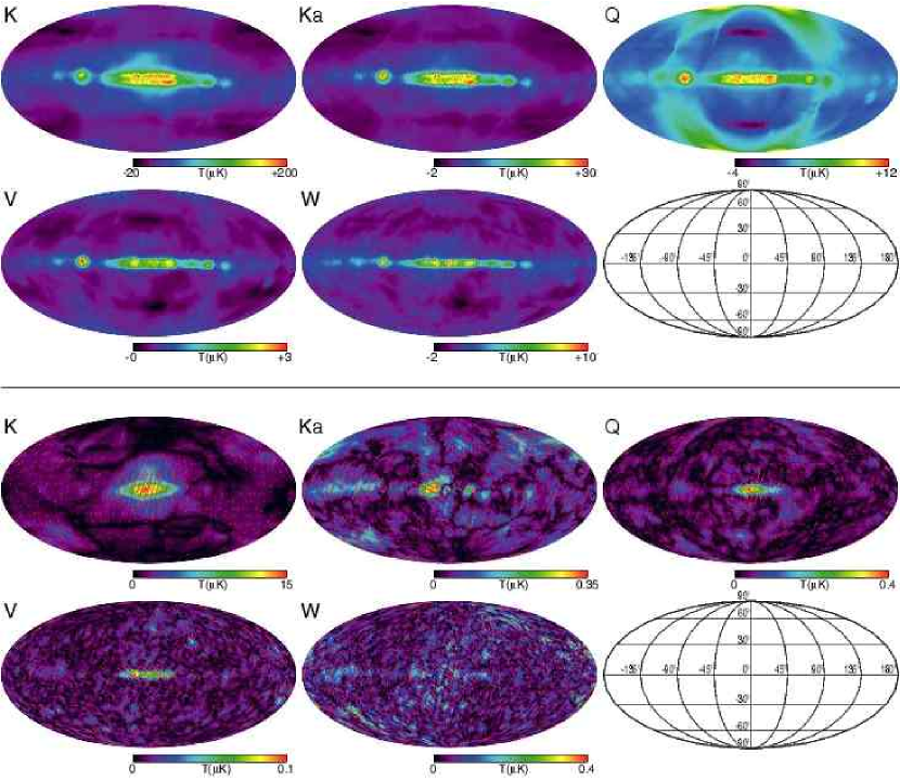
Figure 3: Top: Unpolarized sidelobe pickup contamination for selected sky maps. For purposes of CMB analysis, sidelobe contributions far from the Galactic plane are most important. Bottom: Polarized sidelobe contamination of the CMB maps. Intensity $(Q^{2}+U^{2})^{1/2}$ is shown as a color scale, while polarization directions appear as red lines. These are sidelobe contamination maps, and should not be used to extract information about the polarized microwave sky. They are dominated by signal from the radiometer bandpass mismatch. A higher quality rendering is available on the LAMBDA web site.

Figure LABEL:unpol_spectrum shows angular power spectra for the sidelobe pickup contamination for each DA. Each spectrum is dominated by its lowest $\ell$ components, $0\leq\ell\mbox{${}_{<}\atop{}^{\sim}$}10$. With the exception of K-band, the spectra lie below $\sim 5(\mu\rm K)^{2}$. Since the true sky signal dominates over the sidelobe contamination in every band, the cross-correlation between the sidelobe-pickup maps and the CMB is more relevant. The $C_{\ell}$ are extracted from

$$T_{\rm map}=T_{\rm sky}+T_{\rm contam}+{\rm noise}\ ,$$ (18)

so for a small contamination signal, the leading effect in the power spectrum comes from the $T_{\rm sky}\times T_{\rm contam}$ term. These cross-correlations are shown in Figure LABEL:unpol_crosscorr. K-band shows a contribution around $100\ (\hbox{$\mu$K})^{2}$ at low $\ell$, while all other bands are below $20\ (\hbox{$\mu$K})^{2}$.

3.2 Polarized Sidelobe Pickup

Extracting polarized pickup due to sidelobes is similar to the unpolarized case, although the process is more involved. There are two channels of differential data per pair of feed horns, each one differencing one polarization from the A-side horn with the opposite polarization from B-side. That is, the signals are: $X1=(A_{-}-B_{|})$ and $X2=(A_{|}-B_{-})$, where $A_{|(-)}$ is power entering the radiometer from the $|$ $(-)$ polarized arm of the OMT on the A-side feed horn, and similarly for $B_{-(|)}$. The unpolarized signal channel is $X1+X2$, while the purely polarized signal is

$$X1-X2=(A_{-}-A_{|})-(B_{|}-B_{-})\ .$$ (19)

If the antenna patterns of the two perpendicular polarizations seen through the same feed horn were different on the sky, unpolarized pickup of a varying sky could be misidentified as a polarized signal. Fortunately, the sidelobe gain patterns closely match for the two opposite polarizations, in both measurements and models. That is

$$g_{X-}({\bf n}) = g_{X|}({\bf n})\ ,\quad{\rm and}$$ (20)

$$\mbox{\boldmath$P$}_{X-}({\bf n}) = {\bf n}\times\mbox{\boldmath$P$}_{X|}\ ,$$ (21)

for all ${\bf n}$, to within the uncertainties of the models and measurements. A direct test of this match was to take a polarized source, measure the gain pattern through one arm of a feed horn OMT, rotated the source by 90^∘and switch the receiver to the other arm of the OMT, and repeated the measurement. This always generated the same antenna pattern up to measurement uncertainty. Small main beam deviations from equation (21) were observed; these are reported and discussed in Page et al. (2003a).

There is, however, a mechanism by which unpolarized foreground pickup can induce a polarized signal, equation (19). The mismatch comes not in the optics, but in the broadband radiometer gains, $r_{{}_{X1}}(\nu),\ r_{{}_{X2}}(\nu)$. The radiometers are separately calibrated on the CMB dipole, and so will agree on any CMB signal. However, if a source has a different spectrum, for example a steeply non-thermal $T_{\rm sky}({\bf n},\nu)\propto\nu^{\alpha-2}$ (Page et al., 2003a), with $\alpha-2$ significantly far from zero, then any mismatch in radiometer gains can generate a spurious polarization signal:

$$\delta T_{{\rm pol},X}^{\rm spr}=\int\,{\rm d}\nu\,\left(r_{{}_{X1}}(\nu)-r_{{}_{X2}}(\nu)\right)T_{\rm sky}^{\rm nt}(\nu)\ .$$ (22)

Here $T_{\rm sky}^{\rm nc}$ is any non-CMB sky signal, and spacecraft orientation and the integral over the sky have been suppressed. The signal in equation (22) comes from inherently unpolarized foreground sources, and so pickup from it is independent of the spacecraft polarization direction, i.e., there is no $\mbox{\boldmath$P$}_{\rm sky}\cdot{\cal O}^{\top}\mbox{\boldmath$P$}_{X}\sim\cos(2\Phi_{\rm sc,sky})$ dependence in equation (22). In the limit of even sampling over all spacecraft orientations, main beam pickup of this uniform signal would not contribute to the polarization maps. However, the non-uniformity of the actual set of spacecraft orientations does cause this main-beam spurious pickup to leak into the polarization maps; see Kogut et al. (2003) for a full discussion.

Through sidelobe pickup, however, this spurious polarization signal directly contributes to the polarized maps, even where spacecraft orientation is sampled uniformly. When the A-side main beam points at a particular pixel, the sidelobe pickup from equation (22) will naturally vary with spacecraft orientation $\Phi$, since the sidelobes will swing across the foregrounds as the spacecraft is rotated about the main-beam axis. This spurious pickup must be included along with the pickup from polarized sources to calculate the sidelobe-induced foreground contamination of our polarization maps. Fortunately it is possible to accurately calculate this pickup for each radiometer. If one takes the polarized radiometer signal, equation (19), from the time ordered data, and then runs it through the unpolarized map-making algorithm, one obtains a full sky map:

$$T_{{\rm pol},X}^{\rm spr}({\bf n})=\left[\mbox{Map-making}\right]\circ(X1-X2)_{\rm TOD}\ ,$$ (23)

which is composed purely of the spurious polarization signal for the radiometer pair $X1,X2$. Genuine polarized pickup enters the time ordered data of $(X1-X2)$ equally with opposite signs, and so is null in of equation (23). The sidelobe pattern can then be folded back in with this sky map for each radiometer pair to calculate the spurious signal for any spacecraft orientation.

Polarized sidelobe pickup results from two sources: polarized sky signal in polarized sidelobes, and radiometer RF band mismatch on foregrounds. The most significant pickup comes from the bright plane of the Galaxy and the band mismatch, followed by the strongly polarized foregrounds in the plane, a couple of supernova remnants, and the Northern Galactic Spur.

To generate maps of sidelobe-induced contamination in the sky maps, again we start with the existing year one polarized sky maps, for each horn pair (a single differencing assembly). When the telescope is in orientation ${\cal O}$, the polarized sky signal it sees through the sidelobes is:

$$\delta T_{\rm pol,\mit X}({\cal O})={1\over 4\pi}\int\,{\rm d}\Omega_{\bf n}\ g_{X}({\cal O}{\bf n})T_{\rm pol,\mit X}({\bf n})\times$$

$$\biggl{[}\left(\mbox{\boldmath$P$}_{\rm sky,\mit X}({\bf n})\cdot{\cal O}^{\top}\mbox{\boldmath$P$}_{X-}({\cal O}{\bf n})\right)^{2}-$$

$$\left(\mbox{\boldmath$P$}_{\rm sky,\mit X}({\bf n})\cdot{\cal O}^{\top}\mbox{\boldmath$P$}_{X|}({\cal O}{\bf n})\right)^{2}\biggr{]}$$

$$+{1\over 4\pi}\int\,{\rm d}\Omega_{\bf n}\ g_{X}({\cal O}{\bf n})T_{\rm pol,\mit X}^{\rm spr}({\bf n})\ .$$ (24)

Since $\mbox{\boldmath$P$}_{-}$ is everywhere perpendicular to $\mbox{\boldmath$P$}_{|}$, the integral may be written

$$\delta T_{\rm pol,\mit X}({\cal O})={1\over 4\pi}\int\,{\rm d}\Omega_{\bf n}\ g_{X}({\cal O}{\bf n})\times$$

$$\left[T_{\rm pol,\mit X}({\bf n})\cos\left(2\Phi({\bf n},{\cal O})\right)+T_{\rm pol,\mit X}^{\rm spr}({\bf n})\right]\ ,$$ (25)

where $\Phi$ is the angle between incoming sky polarization and antenna pattern polarization, for a particular point on the sky and spacecraft orientation.

Each measurement $\delta T_{\rm pol,\mit X}({\cal O})$ contributes to the recovered polarization of two pixels, the positions of the A and B beam peaks at orientation ${\cal O}$. For polarization, the angle, $\gamma$, between beam peak polarization direction and the chosen set of sky coordinates is also needed. For WMAP ’s maps of the polarized sky, we chose to reference Stokes parameters to the Galactic meridian. Here define $\gamma_{X}({\cal O})$ as the angle from the instrument polarization vector ${\cal O}^{\top}\mbox{\boldmath$P$}_{X}$ to the Galactic meridian.

Tracing the sidelobe pickup $\delta T_{\rm pol,\mit X}({\cal O})$ through the map-making algorithm, the data pipeline receives a set of offsets to measurements of an unknown polarization intensity and direction at a particular pixel, ${\bf n}={\cal O}^{\top}\mbox{\boldmath$A$}_{X}$ or ${\cal O}^{\top}\mbox{\boldmath$B$}_{X}$. These values correspond to a series of $n$ measurements of a local Stokes $Q$ parameter, in a frame rotated by an angle $\gamma_{A(B),X}({\cal O})$ from the frame where we wish to extract $Q$ and $U$. That is, it sees a series of $n$ measurements $Q_{i}$:

$$\left[\begin{array}[]{c}Q_{1}\\ Q_{2}\\ \vdots\\ Q_{n}\end{array}\right]=\left[\begin{array}[]{cc}\cos 2\gamma_{1}&-\sin 2\gamma_{1}\\ \cos 2\gamma_{2}&-\sin 2\gamma_{2}\\ \vdots&\vdots\\ \cos 2\gamma_{n}&-\sin 2\gamma_{n}\end{array}\right]\left[\begin{array}[]{c}Q\\ U\end{array}\right]\ ,$$ (26)

where $Q,U$ are the unknown, desired values. The values of $Q,U$ which best fit this data set are:

$$\left[\begin{array}[]{c}Q\\ U\end{array}\right]=M^{-1}\sum_{i}\left[\begin{array}[]{r}Q_{i}\cos 2\gamma_{i}\\ -Q_{i}\sin 2\gamma_{i}\end{array}\right]\ ,$$ (27)

where

$$M=\sum_{i}\left[\begin{array}[]{rr}\cos^{2}2\gamma_{i}&-{1\over 2}\sin 4\gamma_{i}\\ -{1\over 2}\sin 4\gamma_{i}&\cos^{2}2\gamma_{i}\end{array}\right]\ .$$ (28)

This is a linear system, so the induced sidelobe pickup travels through the mapmaking procedure independently from any main beam signal. After generating a family of $\delta T_{\rm pol,\mit X}({\cal O})$ by performing the integrals in equation (25), one can then construct the induced contributions to the $Q$ and $U$ maps.

$$\left[\begin{array}[]{c}\delta Q^{\rm ind}_{X}({\bf n})\\ \delta U^{\rm ind}_{X}({\bf n})\\ \end{array}\right]\simeq{1\over 2}\left[\begin{array}[]{c}\delta Q_{A,X}({\bf n})+\delta Q_{B,X}({\bf n})\\ \delta U_{A,X}({\bf n})+\delta U_{B,X}({\bf n})\\ \end{array}\right]\ ,$$ (29)

where

$$\left[\begin{array}[]{c}\delta Q_{A,X}({\bf n})\\ \delta U_{A,X}({\bf n})\\ \end{array}\right]={1\over 2}M^{-1}_{A,X}\times\hbox{\hskip 72.26999pt}$$ (32)

$$\sum_{i}\left[\begin{array}[]{r}\delta T_{\rm pol,\mit X}({\cal O}_{i})\cos\left(2\gamma_{{}_{A,X}}({\cal O}_{i},{\bf n})\right)\\ -\delta T_{\rm pol,\mit X}({\cal O}_{i})\sin\left(2\gamma_{{}_{A,X}}({\cal O}_{i},{\bf n})\right)\end{array}\right]\ ,$$ (35)

and similarly for the B side, with the sign of $\delta T_{\rm pol,\mit X}({\cal O})$ reversed. Here $M_{A,X}$ is defined as in equation (28), for the set of angles: $\left\{\gamma_{{}_{A,X}}({\cal O}_{i},{\bf n})\right\}$. All ${\cal O}_{i}$ preserve the pixel whose polarization is under study: ${\cal O}_{i}{\bf n}={\bf n}$. As for the unpolarized maps, it is crucial to use the same family of ${\bf n}_{i}$ present in the actual observations in the first year scan pattern. The new factor of $1/2$ in equation (35) comes from the map-making assumption that one half of the measured signal comes from each side.

In the end, equation (35) approximates the polarized sidelobe pickup with a method precisely analogous to equation (10) for overall power. From the existing microwave maps and antenna patterns, one creates a family of simulated measurement differences $\delta T_{\rm pol}$, and then propagates them through one iteration of the map-making algorithm. As before, to propagate the simulated data through the full map-making data pipeline is a task for the next generation of data analysis.

3.2.1 Results for Polarized Sidelobe Pickup

The lower portion of Figure LABEL:allmaps shows the sidelobe contamination in one map for each band. The “spurious” pickup due to radiometer bandpass mismatch slightly dominates true polarized pickup, and so the Galaxy, appearing as a coherent, polarized source, dominates the images. Even the brightest sidelobe contamination is extremely weak: the Galaxy peaks at $\sim 400$ nK in all bands except K, where a stronger band mismatch leads to a 16 $\mu$K signal in the plane.

DA	Mean	Min	Max	rms
	($\mu$K)	($\mu$K)	($\mu$K)	($\mu$K)
K1	0.8	$7\times 10^{-3}$	5	1.0
Ka1	$3\times 10^{-2}$	$3\times 10^{-4}$	0.13	$4\times 10^{-2}$
Q1	$1.6\times 10^{-2}$	$8\times 10^{-5}$	$9\times 10^{-2}$	$2\times 10^{-2}$
Q2	$3\times 10^{-2}$	$9\times 10^{-5}$	0.3	$5\times 10^{-2}$
V1	$2\times 10^{-3}$	$3\times 10^{-5}$	$1.4\times 10^{-2}$	$3\times 10^{-3}$
V2	$2\times 10^{-3}$	$3\times 10^{-5}$	$1.4\times 10^{-2}$	$2\times 10^{-3}$
W1	$6\times 10^{-2}$	$9\times 10^{-5}$	0.5	$7\times 10^{-2}$
W2	$4\times 10^{-2}$	$4\times 10^{-4}$	0.2	$5\times 10^{-2}$
W3	$4\times 10^{-2}$	$4\times 10^{-4}$	0.2	$5\times 10^{-2}$
W4	$8\times 10^{-2}$	$1.0\times 10^{-3}$	0.5	$9\times 10^{-2}$

Table 2: Contamination of the polarized maps due to sidelobe pickup. Averages are taken outside of the Kp0 mask region, away from the Galaxy.

Table 2 shows means for the sidelobe contamination of each Q,U pair of polarized maps. With the exception of K-band, where a stronger bandpass mismatch leads to a polarized signal ranging to 5 $\mu$K outside of the Kp0 mask, expected contamination per pixel is $\mbox{${}_{<}\atop{}^{\sim}$}400$ nK. Angular power spectra for the intensity of polarized sidelobe contamination are shown in Figure LABEL:pol_spectrum.

Again, the power spectrum of the sidelobe contamination itself is less interesting than its cross-correlation with the CMB. Polarized sidelobe pickup contributes to the TE power spectrum, most strongly via the term $T_{\rm sky}\times E_{\rm contam}$, where $E_{\rm contam}$ is generated from the $Q$ and $U$ sidelobe contamination maps. Applying the same analysis as is used for the microwave sky TE power spectrum (Kogut et al., 2003), one can calculate the sidelobe-induced contribution to the WMAP year one TE spectra. The CMB $\times$ polarized sidelobe map TE spectra are shown in Figure LABEL:TE_spectrum. In K-band, sidelobe polarization pickup generates a TE signal comparable to our reported value, $\ell|X_{\ell}|$ ranges from 1 to 10 $\hbox{$\mu$K}^{2}$. For all other bands,, the cross-correlation angular power $\ell|X_{\ell}|$ ranges from .03 to 0.5  $\hbox{$\mu$K}^{2}$, with a roughly flat spectrum. K-band polarization maps are corrected for sidelobe pickup before they are used to calculate CMB spectra. For all other bands, sidelobe contamination is a subdominant contributor to the TE spectrum error.

Figure 4: Angular power spectra of sidelobe contamination maps for the WMAP year one sky maps. A CMB angular power spectrum is shown in black for comparison. All spectra shown were made with the Kp0 Galaxy+source mask (Bennett et al., 2003b).	Figure 5: Absolute value of the cross-correlation between sidelobe pickup and the microwave sky. This is the extent to which sidelobe contributions should contaminated calculated $C_{\ell}$ values. A CMB power spectrum is shown in black for comparison.
Figure 6: Angular power spectra for polarized sidelobe contamination. These are spectra for the intensity of the polarized pickup; $P_{\ell}$ is the angular power of $(\delta Q^{2}+\delta U^{2})^{1/2}$, for each radiometer pair. Both bandpass mismatch and polarized foreground pickup are included. This spectrum is not one generally used for CMB analysis, but serves to show the strength and angular dependence of the polarized sidelobe contamination.	Figure 7: The TE angular power spectra for polarized sidelobe contamination. These are the largest sidelobe contribution to the WMAP year one TE spectra, from the $(\delta Q,\delta U)_{\rm sidelobes}\times(\delta T_{\rm cmb})$. The WMAP reported CMB TE spectrum is shown in black for comparison. After corrections for Galactic foreground pickup, direct radiometer bandpass mismatch, and polarized sidelobe pickup (K-band only), K—W-band data was used to generate the reported TE spectrum at low $\ell$. Omitting K-band changes the reported spectrum very little (Kogut et al., 2003).

4 Discussion

For both unpolarized and polarized microwave sky maps, the above techniques yield measures of the sidelobe contamination in each map accurate to $\sim$ 30%. Most of this uncertainty comes from the overall calibration error in the sidelobe gains, although a few percent may be attributed to the approximations in equations (10), (17), and (29), (35). With the information available, improvements are possible in a second round of analysis.

The first improvement will be with the calibration of the sidelobe maps. With sidelobe maps for all ten horn positions, and with high-quality sky maps now available, we can return to the differential time ordered data and extract a best fit calibration for each gain pattern. Using the time ordered $\delta T_{X}({\cal O})$, we can bypass the various approximations made in §3.1, §3.2. Using the time ordered data, one can calibrate sidelobe gains directly from the sky maps, and then correct the data stream directly, prior to map-making. Wandelt & Górski (2001) have proposed a mechanism to perform this calculation efficiently on large data sets.

It appears possible that their method can eliminate sidelobes to below 5% of their original strength. A similar correction is possible for the polarized sidelobe pickup.

4.1 Conclusion

The systematic signal in the one-year WMAP data induced by sidelobe pickup of the Galaxy is small. The sidelobes do not contribute strongly to the uncertainties in the CMB anisotropy maps, or in the TE angular cross power spectrum. Since the sidelobes are broad, smooth features on the sky, their influence is important only at the largest angular scales, $\ell<20$. Outside of the Galactic region, the magnitude of overall sidelobe pickup ranges from $60\ \mu\rm K$ in K-band to $1\ \mu\rm K$ in V and W-bands. Polarized sidelobe pickup is markedly smaller, ranging from $1\mu\rm K$ in K-band down to a few nK at higher frequencies.

For the first year WMAP results we restrict ourselves to calculating sidelobe contamination using the approximations discussed here. We subtract a sidelobe signal only from the K-band maps. In future data sets, we plan to use the raw time ordered data to directly calibrate the sidelobe maps, and subsequently correct the time-stream data to remove sidelobe pickup from future maps.

References

- Barnes et al. (2002) Barnes, C., Limon, M., Page, L., Bennett, C., Bradley, S., Halpern, M., Hinshaw, G., Jarosik, N., Jones, W., Kogut, A., Meyer, S., Motrunich, O., Tucker, G., Wilkinson, D., & Wollack, E. 2002, ApJS, 143, 567
- Bennett et al. (2003a) Bennett, C. L., Bay, M., Halpern, M., Hinshaw, G., Jackson, C., Jarosik, N., Kogut, A., Limon, M., Meyer, S. S., Page, L., Spergel, D. N., Tucker, G. S., Wilkinson, D. T., Wollack, E., & Wright, E. L. 2003a, ApJ, 583, 1
- Bennett et al. (2003b) Bennett, C. L., Halpern, M., Hinshaw, G., Jarosik, N., Kogut, A., Limon, M., Meyer, S. S., Page, L., Spergel, D. N., Tucker, G. S., Wollack, E., Wright, E. L., Barnes, C., Greason, M., Hill, R., Komatsu, E., Nolta, M., Odegard, N., Peiris, H., Verde, L., & Weiland, J. 2003b, ApJ, submitted
- Bennett et al. (1992) Bennett, C. L., Smoot, G. F., Janssen, M., Gulkis, S., Kogut, A., Hinshaw, G., Backus, C., Hauser, M. G., Mather, J. C., Rokke, L., Tenorio, L., Weiss, R., Wilkinson, D. T., Wright, E. L., de Amici, G., Boggess, N. W., Cheng, E. S., Jackson, P. D., Keegstra, P., Kelsall, T., Kummerer, R., Lineweaver, C., Moseley, S. H., Murdock, T. L., Santana, J., Shafer, R. A., & Silverberg, R. F. 1992, ApJ, 391, 466
- Bennett et al. (2003c) Bennett, C. L. et al. 2003c, ApJ, submitted
- Hinshaw et al. (2003a) Hinshaw, G. F. et al. 2003a, ApJ, submitted
- Hinshaw et al. (2003b) —. 2003b, ApJ, submitted
- Kogut et al. (2003) Kogut, A. et al. 2003, ApJ, submitted
- Page et al. (2003a) Page, L. et al. 2003a, ApJ, submitted
- Page et al. (2003b) —. 2003b, ApJ, 585, in press
- Rahmat-Samii et al. (1995) Rahmat-Samii, Y., Imbriale, W., & Galindo-Isreal, V. 1995, DADRA, YRS Associates, rahmat@ee.ucla.edu
- Wandelt & Górski (2001) Wandelt, B. D. & Górski, K. M. 2001, Phys. Rev. D, 36, 123002