Strong and weak lensing united III: Measuring the mass distribution of the merging galaxy cluster 1E065756 **affiliation: Based on observations made with the NASA/ESA Hubble Space Telescope, obtained at the Space Telescope Science Institute, which is operated by the Association of Universities for Research in Astronomy, Inc., under NASA contract NAS 5-26555. These observations are associated with program # 10200. This work is also based in part on observations made with the Spitzer Space Telescope and with the 6.5 meter Magellan Telescopes located at Las Campanas Observatory, Chile. Spitzer is operated by the Jet Propulsion Laboratory, California Institute of Technology under a contract with NASA.
Abstract
The galaxy cluster 1E0657-56 () is remarkably well-suited for addressing outstanding issues in both galaxy evolution and fundamental physics. We present a reconstruction of the mass distribution from both strong and weak gravitational lensing data. Multi-color, high-resolution HST ACS images allow detection of many more arc candidates than were previously known, especially around the subcluster. Using the known redshift of one of the multiply imaged systems, we determine the remaining source redshifts using the predictive power of the strong lens model. Combining this information with shape measurements of “weakly” lensed sources, we derive a high-resolution, absolutely-calibrated mass map, using no assumptions regarding the physical properties of the underlying cluster potential. This map provides the best available quantification of the total mass of the central part of the cluster. We also confirm the result from Clowe et al. (2004, 2006a) that the total mass does not trace the baryonic mass.
Subject headings:
cosmology: dark matter – galaxies: clusters: general – gravitational lensing – galaxies:clusters:individual:1E0657-561. Introduction
The cluster of galaxies 1E065756 is one of the hottest, most X-ray luminous clusters known. Since its discovery by Tucker et al. (1995), it has been the subject of intense and ongoing research (Mehlert et al. 2001, Markevitch et al. 2002, Barrena et al. 2002, Clowe et al. 2004, Markevitch et al. 2004, Gomez et al. 2004). In particular, Chandra observations by Markevitch et al. (2002) revealed the cluster to be a supersonic merger in the plane of the sky with a textbook example of a bow shock, making this cluster a unique case in which to study hydrodynamical properties of interacting systems. The optical images show that the cluster has two distinct components, and the X-ray analysis reveals that the lower mass sub-cluster has recently exited the core of the main cluster with a relative velocity of . Although this relative velocity appears to be unusually large, an analysis of cosmological simulations demonstrates that it is well within the predicted range of the currently favored cosmological model (Hayashi & White 2006).
Due to its unique geometry and physical state, this cluster is the best known system in which to test the dark matter hypothesis (Clowe et al. 2004). The observed offsets between the weak gravitational lensing mass peaks and the X-ray gas component give the most direct evidence for the presence of dark matter yet available. Using the same observations, Markevitch et al. (2004) placed upper limits on the dark matter self-interaction cross section.
The goal of this work is to obtain a high-resolution, absolutely calibrated mass map with no assumptions on the physical properties of the underlying cluster potential. For this purpose we use HST ACS data, incorporating the gravitational lensing information from both multiple image systems (strong lensing) and from distortions of background sources (weak lensing). The superb spatial resolution delivered by ACS both increases the number density of background sources that can be used for weak lensing and reveals new strong lensing candidates, especially around the subcluster. The joint strong and weak lensing analysis thus benefits greatly from the ACS data, enabling us to increase the spatial resolution and signal strength of the mass map in the core of the cluster.
Encouraged by the success of the combined strong and weak lensing reconstruction method developed in Bradač et al. (2005b) (hereafter Paper I) and the results from applying the method to cluster RX J1347.51145 (Bradač et al. 2005a), we proceed to apply this method to 1E065756. Because the strong lensing data are richer in this case (RX J1347.51145 has not been observed with either the ACS or WFPC2 cameras prior to this study), we improve the method as described in the text.
We perform the reconstruction in the following sequence. Using ACS (multi-color where available) HST images, we identify the multiply imaged systems. Having a spectroscopic redshift for one lensed system (from Mehlert et al. 2001), we then use the predictive power of simple strong lens modeling to estimate the redshifts of the other systems. Using positions and redshifts of the strongly lensed images and the shape measurements of the “weakly” lensing sources, we perform a combined strong and weak lensing mass reconstruction, thereby significantly improving the constraints on the mass and positions of the main cluster and the colliding subcluster of 1E065756. In terms of the structure of this paper, in section 2 we describe the optical images used in this analysis, the basic image processing and the extraction of the strong (§2.1) and weak (§2.2) gravitational lensing data. We then infer the mass distribution of cluster 1E065756 from these data in section 4, following a demonstration of our methodology on suitable simulated data in section 3. We discuss the possible sources of error in section 5 and summarize our conclusions in section 6.
2. Observations and data reduction process
ACS/WFC imaging of the cluster 1E065756 was carried out in Cycle 13 (proposal 10200, PI Jones) on 2004 October 21 in two pointings with one and three different filters respectively. The two pointings are centered on the main cluster and the subcluster with a small overlap between them. The subcluster was observed in three different filters (three orbits with F814W, one with F606W, and one with F435W), while the main cluster was observed only in the F606W filter (one orbit).
The demands placed by the lensing analysis require special care when reducing the images. We use the Multidrizzle (Koekemoer et al. 2002) routine to align the images. To register the images with the astrometric accuracy needed for lensing analysis, we determine the offsets among the images by extracting high objects in the individual, distortion corrected exposures. We use Sextractor (Bertin & Arnouts 1996) and the IRAF routine geomap to identify the objects and calculate the residual shifts and rotation of individual exposures, which were then fed back into Multidrizzle. We use “square” as the final drizzling kernel and an output pixel scale of ; this is smaller than the original pixel scale of the ACS CCD to reduce the impact of resampling on the shape measurements.
2.1. Strong lensing image identification
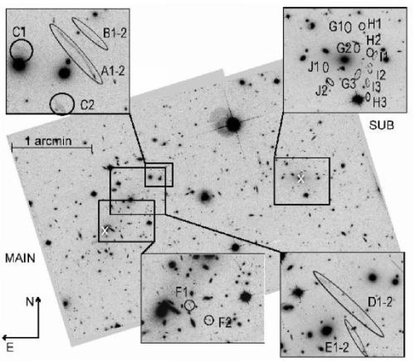
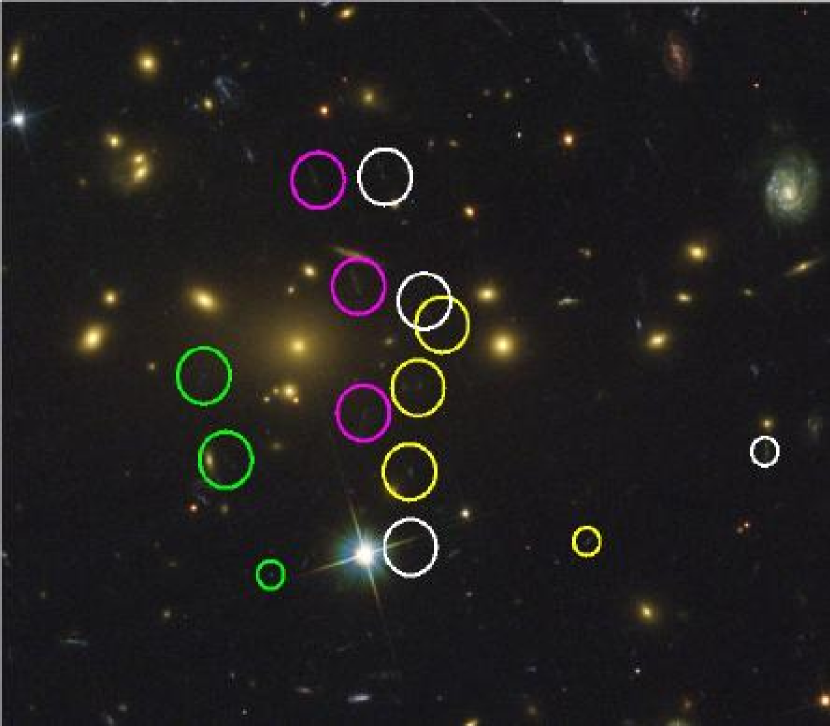
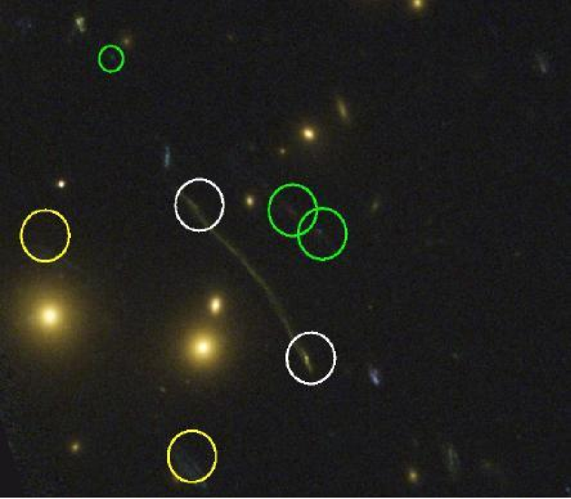
Owing to its complex structure, the strong lensing analysis of the 1E065756 cluster is complicated. Among the multiply-imaged systems, only the giant arc on the NW side of the main cluster’s cD has a measured redshift ( Mehlert et al. 2001). Corresponding images for multiply-imaged sources were identified by matching both morphologies and surface brightnesses in each of the available ACS bands (F435W, F606W, and F814W) and ground-based filters, BVR data from Magellan and I-band from VLT (Clowe et al. 2004).
We confirm (based on photometry and morphology) that the systems (labeled A-F in Table 1) previously identified by Mehlert et al. (2001) are indeed multiply imaged. We identify four additional systems (G-J) in the subcluster region, where none were previously known. All of these are identified in Fig. 1, and image positions (corresponding to the peak surface brightness) are presented in Table 1. Unfortunately, for the greater part of the main cluster, only a single band ACS image is available, which makes identification of additional candidates significantly more ambiguous.
Using these identifications, we perform a parametrized strong lensing reconstruction. At this stage we are not generating a detailed strong lensing model, rather we use this parametrized model only to predict the redshifts of the systems where spectroscopic redshifts are not available (all systems but A) and as the initial model guess for the subsequent strong and weak lensing reconstruction. For this reconstruction, we use only the image positions as constraints. The parametrized model consists of two non-singular isothermal ellipses (NIE) (Keeton & Kochanek 1998), for which the scaled surface mass density is given by
| (1) |
is defined counterclockwise from due west and is related to the line-of-sight velocity dispersion through . The components are centered on the southern cD galaxy of the main cluster and the brightest cluster galaxy (BCG) of the sub cluster respectively (denoted with white crosses in Fig. 1; it is not straightforward to identify the BCG of the main cluster, therefore we refer to the two main galaxies as the southern and northern cD). We allow the scaling , core radii , ellipticities , and position angles of these to vary.111We define all ellipticities throughout this paper as in Bartelmann & Schneider (2001) with , being the axes ratio. Following the prescription of Kneib et al. (1996), we also include the 20 brightest cluster members from the F606W-band (selected using color information from Magellan data) in the mass model. The galaxies are modeled as non-singular isothermal spheres with a line-of-sight velocity dispersion and core radius following
| (2) |
The proportionality constants are allowed to vary as well and below we quote the values of and for a fiducial galaxy with a F606W-band magnitude . The best fit model for this system has values of for the main cluster, for the subcluster, and for the cluster members. We also allow the redshifts of systems B-J to vary. The resulting best fit redshifts are given in Table 1. To evaluate the angular diameter distances throughout the paper we assume the CDM cosmology with , , and Hubble constant .
For objects close in projection to the main cluster, the redshift estimates are fairly reliable because the well-measured arc A is located there (we estimate an error of ). However, the redshift estimates for those close to the subcomponent are less well-determined, and are somewhat degenerate with the adopted mass of the subcluster. We postpone an extension of the methodology described in the following sections that incorporates simultaneous solution for the unknown source redshifts to future work, but here note that: 1) the parametrized model allows the generation of a set of source redshifts that, while model-dependent, are self-consistent; 2) the predicted redshifts are consistent with the colors of the objects. We adopt the redshifts estimated here for the combined strong and weak lensing reconstruction, and where possible estimate the systematic error introduced as a result of this simplification.
| Ra | Dec | ||
|---|---|---|---|
| 104.63316 | -55.941395 | ||
| A | 104.62988 | -55.943798 | 3.24222The redshift of arc A was determined spectroscopically by Mehlert et al. (2001). Other redshifts are determined using the best-fit strong lensing model. |
| 104.62954 | -55.941844 | ||
| B | 104.63042 | -55.941474 | 4.8 |
| 104.63775 | -55.941851 | ||
| C | 104.63338 | -55.945324 | 2.1 |
| 104.64709 | -55.943575 | ||
| D | 104.63528 | -55.951836 | 1.4 |
| 104.64008 | -55.950620 | ||
| E | 104.64232 | -55.948784 | 1.0 |
| 104.65155 | -55.956671 | ||
| F | 104.64778 | -55.958284 | 0.8 |
| 104.56568 | -55.939832 | ||
| G | 104.56402 | -55.942113 | 1.3 |
| 104.56417 | -55.944131 | ||
| 104.56293 | -55.939764 | ||
| H | 104.56133 | -55.942430 | 1.9 |
| 104.56189 | -55.947724 | ||
| 104.56186 | -55.946114 | ||
| I | 104.56052 | -55.942930 | 2.1 |
| 104.56141 | -55.944264 | ||
| 104.56909 | -55.946016 | ||
| J | 104.57025 | -55.944050 | 1.7 |
2.2. Weak lensing catalogs
In the weak lensing analysis, we use the F435W, F606W, and F814W exposures for the subcluster, and F606W wherever multicolor ACS data are not available. We will only outline the main steps used for this analysis, full details on how the weak lensing catalogs were generated will be given in a future paper dealing with the weak lensing mass measurements of 1E065756 at large radius (Clowe et al. 2006c, in prep.).
We correct galaxy images for the PSF anisotropy and PSF smearing closely following the technique described in Clowe et al. (2006b). The procedure is based on the KSB algorithm (Kaiser et al. 1995), in particular we use the modified IMCAT implementation. The KSB method is formally valid only in the weak lensing regime (i.e. at radii much larger than where multiply imaged systems form and where the distortions are small). However recent simulations from the STEP project (Heymans et al. 2006) show that this approach is also valid in the non-weak lensing regime (i.e. with shear values of ) to the accuracy needed for a single cluster reconstruction. Lastly, in the vicinity of the highly elongated arcs we are dominated by the strong lensing signal, thereby minimizing the effects of signal dilution due to imperfect PSF correction.
We select stars from the half-light-radius vs. magnitude diagram and fit a fifth order polynomial to their measured ellipticities as a function of their position on the drizzled image. After the correction the rms of the stellar ellipticity components and (as defined in Bartelmann & Schneider (2001)) changes from to and from to , respectively, and the mean is shifted to in both cases. The shear is then measured independently in all available filters and a weighted average is calculated from those to arrive at our final, PSF corrected ellipticity estimates. We use the overlap between the two F606W pointings to test for systematics in the PSF correction. The differences in the shears derived from the two exposures is consistent given the noise level.
The ACS camera has a PSF that varies both spatially and temporally. While the approach described above accounts for the spatial dependence, it does not account for time variations. We investigate the PSF time dependence by measuring stellar shapes in individual exposures (four exposures were taken within each orbit). We conclude that the PSF is not stable (i.e. the global pattern of the PSF changes) even within a single orbit. However our detected signal is much stronger than the typical residuals due to imperfect PSF removal caused by the temporal variation; therefore we use the combined images to measure shapes. In addition, the PSF shape of an individual star changes as a function of its radius (see e.g. Heymans et al. 2005, Jee et al. 2006); we therefore match the radius used to measure the stellar correction factors with that for the galaxies. Using simulated weak lensing data we identified a constant bias between the measured and estimated shear values; this bias was calculated for each image set separately and was introduced as a multiplicative shear calibration factor when producing final catalogs.
The color cuts applied to each catalog to remove cluster and foreground galaxies were color-color cuts estimated using photometric-redshift templates of galaxies at redshifts . We used templates of all but extreme starburst galaxies, under the assumption that there are not likely to be many faint, low-redshift starburst dominated galaxies, particularly in a cluster. As such, we expect that unless there is an unknown population of dwarf galaxies in the cluster with colors much different from known populations, we will have removed all but a handful of outliers (extreme starbursts or dust obscured). We only use objects which were detected in more than a single band; in particular we reject all the objects that are detected only in the F606W pointing of the main cluster and were too faint for detection in the Magellan images.
Unfortunately the observations at hand do not allow us to determine the photometric redshifts of the sources used for weak and strong lensing. We would need at least NIR data to reliably determine the redshifts, as most of the sources are located at . Therefore following Clowe et al. (2006b), we estimate the redshifts of the background sources by applying the color and magnitude cuts that remove the likely foreground population to the HDF-S photometric redshift catalog of Fontana et al. (1999). For the remaining sources, we average the ratios (where , , and are the angular diameter distances to the cluster, source and between the cluster and the source respectively) to generate a very crude estimate of the individual redshifts, but good average redshifts per population (provided the redshift distribution of the HDF-S is representative of that of our background sources). As a result all of the galaxies in a certain magnitude bin will be given the same redshift. The main reason of this approach, instead of calculating a mean for the whole catalog is the fact that the images have different depths in different parts of the reconstructed area, and this method allows us to account for the sudden jumps in the mean background galaxy redshift across the image boundaries, which would otherwise introduce spurious features in the reconstructions.
This method is only approximate, therefore we test the reconstruction method using mock catalogs with only limited knowledge of the redshift of the source population in Sect. 3. The weak and strong lensing reconstruction performs well under these conditions. In addition, any significant dilution of the signal will be compensated by the strong lensing signal (if more than one strong lensing system is used). The cluster is also at a moderate redshift, therefore changing the sources from redshifts of to would change the lensing strength by . In conclusion we expect the contributions due to errors in the assumed distribution of to be smaller than that expected from the galaxy ellipticity shot noise.
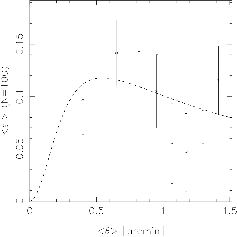
Finally, we fit the non-singular isothermal sphere NIS model to the the averaged tangential ellipticities . Both components generate large tangential shear signal. We center circular bins on the southern cD of the main cluster and the BCG of the subcluster. The resulting NIS fit for the main cluster results in , , and , for the subcluster. This is an oversimplified model because the cluster is morphologically disrupted and we do not correct for the contamination of the main cluster profile in the sub cluster region (and vice versa).

3. Strong and weak lensing reconstruction from high resolution (ACS) data
Our strong and weak lensing reconstruction is performed using the method described in Paper I. The main idea behind the method is to describe the cluster mass distribution using a set of generic model parameters, which we choose to be the projected gravitational potential measured on a regular square grid. The total is defined as
| (3) |
where is the contribution from weak lensing, from strong lensing and is the regularization function with regularization parameter . We closely follow the methodology presented in Paper I, with the few differences described below. 333In figure 2 in Paper I the factor of in finite differencing formula for is wrong. All the calculations in all three papers do however use the correct factor of .
The most important difference is that we extend the formalism to more than a single set of multiple images. This may appear straightforward because we only need to sum up the contributions to from each system. Given multiply imaged systems having images each, we define as
| (4) |
where is the covariance matrix and . is the average position of the -th source (calculated from the image positions and given the deflection angle ), and is the so-called “cosmological weight” function as defined in Bartelmann & Schneider (2001).
In Paper I we assumed that the covariance matrix is diagonal and independent of the lens model parameters. As discussed in e.g. Kochanek (2004), this approach is not optimal and can lead to solutions that are biased toward models that predict high magnification at the image positions. With more sources at differing redshifts, this problem becomes more apparent because the method likely converges toward a solution with steep gradients in the surface mass density close to image positions (allowing for the “fine tuning” of the reconstruction). To overcome such unphysical solutions, we use a better approximation for the error containing the magnification at the image position and obtain the covariance matrix . Such a procedure is approximately correct, provided we are close enough to the true model (see Kochanek 2004). The covariance matrix is still diagonal; however we argue that assuming it to be such in the source plane is in fact a better approximation than assuming the covariance matrix to be diagonal in the image plane, as sources are on average more circular than their lensed images. In addition, in practice multiple image constraints are satisfied nearly perfectly and exact values of errors on image positions are of lesser importance.
We adapt the method to accommodate data regions of arbitrary size and shape, but the potential is reconstructed only in grid cells containing weak and/or strong lensing data. We tile the observed field with a regular grid and determine which cells contain either weak lensing galaxies or multiple images. This can result in some cells being sparsely populated (holes in the data, edge effects), but the regularization ensures that potential is properly reconstructed. Once the data-grid is determined, we ensure that each of the data grid points is surrounded by a grid of points that are included in the reconstruction to calculate the scaled surface mass density , shear , and the deflection angle , using finite differencing, as described in Paper I.
To find the -function minimum, we search for a solution of the following system of equations . This is in general a non-linear set of equations, which we solve in an iterative manner. We again linearize this system as described in Paper I, calculating all of the non-linear terms (for the strong lensing term in particular these are now the ones containing and ) using the information from the previous iteration. We regularize the solution using a “moving prior”, gradually updating our knowledge of the model by increasing its complexity and computing its likelihood relative to the previous (simpler) model. We begin with an initial model (, , ) computed on a relatively coarse grid, and then gradually increase the number of grid points, comparing the resulting map with that from the previous iteration, linearly interpolated onto the finer grid. In addition to we now also use the components of the shear and in the regularizing scheme, to avoid the numerical effects described in Paper I even more efficiently. The regularization constant was set after experimentation with simulated data. When using many multiply imaged systems, the final reconstruction is even less sensitive to these choices than when only a single system is used (as in Paper I); we discuss this finding in more detail in Sect. 5.
With many multiply imaged systems, we must choose a sufficiently fine grid to be able to calculate the difference in the deflection angle between images of different systems (if images from more than one system lie within the same grid cell, it is difficult to find a good solution). Ideally one would like to use adaptive grids for this purpose (having a relatively coarse grid where only weak lensing information is available and increasing the resolution in the vicinity of the multiple images). Unfortunately it is computationally difficult to track such a problem and is therefore beyond the scope of this paper, but will be a subject of future work.
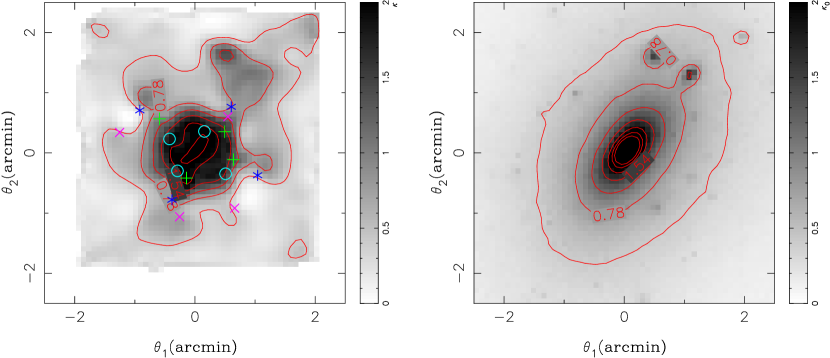
We tested all the improvements described above using a high-resolution N-body simulation of a galaxy cluster by Springel et al. (2001). The catalogs are generated as in Paper I, although adapted to the higher-resolution data that we use here. The weak lensing simulated data are obtained by placing galaxies (giving a density of ) randomly on a field. The intrinsic ellipticities are drawn from a Gaussian distribution, with each component characterized by . We then draw the redshifts of the background sources, following Brainerd et al. (1996), from a gamma distribution with , giving a mean redshift of , and a mode of . We reject the foreground objects, and use the background object redshifts when predicting the lensed shapes. However, when using the catalogs for the reconstruction, we assume no knowledge of the individual redshifts: instead all sources are assumed to have , in agreement with the poor estimates available for the actual data. The multiple-image systems are generated as described in Paper I. Four quadruply-imaged systems are generated at source redshifts of . The initial model for the regularization is set to .
The resulting reconstruction is given in Fig. 3. It is very encouraging to observe how well the overall shape (the agreement in the ellipticity and position angle of the main component, and the overall profile) and its mass are reconstructed. These successes would not be possible with weak lensing data alone, owing to the mass-sheet degeneracy (i.e. the reconstruction would suffer from the degeneracy of the form , where is an arbitrary constant, see e.g. Bradač et al. 2004). In addition with the ACS-quality data, we are starting to resolve the small-scale substructure of the potential.
4. Cluster mass reconstruction of 1E065756
We now apply the above mentioned reconstruction method to the strong and weak lensing data of 1E065756. As described in Sect. 2.1, we use 10 distinct multiply imaged systems and “weakly” lensed galaxies (). We start with a grid for a field oriented with respect to the negative RA coordinate (not all of the grid cells contain data and those that do not are excluded from the reconstruction). We gradually increase the number of grid points (for reasons described in Sect. 3) in steps of 1, with the final reconstruction performed on a grid. In our initial model, we use a two-component NIE model with parameters as given in Sect. 2.1 to set the regularization. The possible dependence of the reconstruction on initial conditions is discussed in the next section.
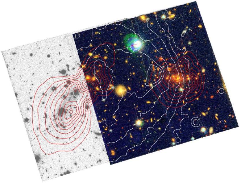
The resulting reconstruction is shown in Fig. 4, together with X-ray surface brightness contours from the 500 ks Chandra observation. The two cluster components are clearly detected. In addition, with superb strong lensing data (due to exquisite ACS resolution and multi-color information for the subcluster) we are starting to resolve multiple components within each individual system.
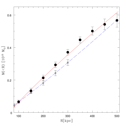
From this reconstruction, we measure the enclosed (projected within a cylinder) mass for this system. The main cluster has , while the sub cluster has ( at the cluster redshift). The mass errors represent combined errors obtained by bootstrap resampling of the weak lensing catalogs, performing a similar experiment for the strong lensing data, and estimating systematic uncertainties from the mass differences obtained using different initial models (see discussion in the next section). We plot the integrated, azimuthally-averaged mass profiles for the two components in Fig. 5. We fit power-law models () to these profiles, and find logarithmic slopes of for the main cluster and for the subcluster. In terms of the surface mass density , this translates to , and . Adopting an isothermal profile (), we find the line of sight velocity dispersions for the main and the sub cluster are and respectively; in good agreement with the analysis in Sect. 2.2. However, as already mentioned in that section, given the size of the errors, the asphericity of the system, and the complicated geometry (the relative contributions of the main and sub cluster are difficult to disentangle), the velocity dispersion and slope measurements should only be used as guidelines.
Because of this cluster’s violent history, we can not expect the assumption of isothermality to hold. Therefore (and for the reasons stated above) it is also non-trivial to compare our velocity dispersion measurements with the ones from Barrena et al. (2002). Their estimate for the main cluster agrees with ours, while the velocity dispersion of a subcluster is much lower in their case. An isolated lens with the low velocity dispersion measured by Barrena et al. (2002) for the subcluster would have multiply imaged systems only at radii , a factor of below that observed. The influence of the main cluster can increase the radial range over which multiple images exist, but not to the extent observed here. We conclude that the true velocity dispersion of the subcluster is likely to be smaller than that derived from our mass model (due to the inclusion of mass from the main cluster), but larger than that presented by Barrena et al. (2002).
One of the important results of the work of Clowe et al. (2004, 2006a) was the measurement of the offset between dark matter and baryons. We confirm these results: our strong and weak lensing offsets for the mass peaks (by measuring the peaks in -distribution) and the corresponding errors are given in Table 2. To estimate the significance of this offset we also measured the positions of the two peaks (for the main and the subcluster) in each of the 1000 reconstructions using the bootstrap resampled weak lensing catalogs (described below). In none of these realizations are the mass peaks coincident with the corresponding X-ray peaks. The 1- error bars are a factor of and smaller than the offsets for the main and subcluster respectively. If these errors are accurate and Gaussian distributed, this result translates into 10- and 6- discrepancies between the corresponding gas and the total mass peaks. These offsets directly demonstrate that dark matter is present and is the dominant mass component of this cluster.
Lastly, we compare the projected gas mass (the details of modeling will be given in Randall et al. 2006) vs. the total mass within elliptical regions centered on the two peaks of the X-ray emission and the southern cD of the main and BCG of the subcluster, respectively (see Table 3). The ratio of gas mass to total mass is smaller in the regions centered on the massive galaxies rather than the X-ray peaks, indicating that the gas has been (to some extent) stripped, and is no longer coincident with the total mass. In addition, we detect an extension in the total mass map to the NW of arc A. This detection can be partly attributed to the hot X-ray gas (see Fig. 4).
| Main component | ||
| Main component (gas) | 1.06 | 0.84 |
| Sub component | ||
| Sub component (gas) | -0.73 | 0.10 |
5. Possible systematic effects
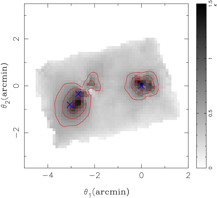
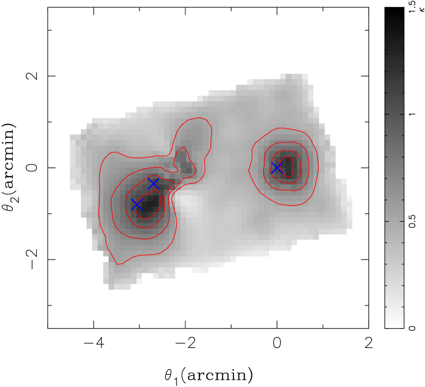
To assess the reliability of the reconstructed map, we generate 1000 bootstrap resampled weak lensing catalogs and perform reconstructions on each of these. To further test the reliability of the strong lensing data we create 10 different reconstructions each time removing one of the multiply imaged systems we use. The resulting -maps do not change substantially, the main features (i.e. the ellipticity of the main and the subcluster) seen in Fig. 4 remain in all of the reconstructions.
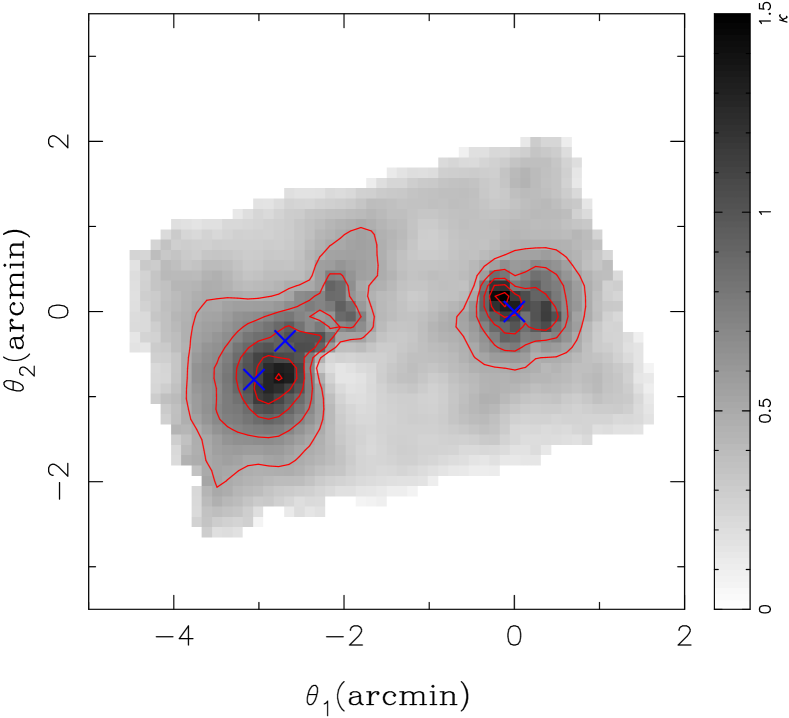
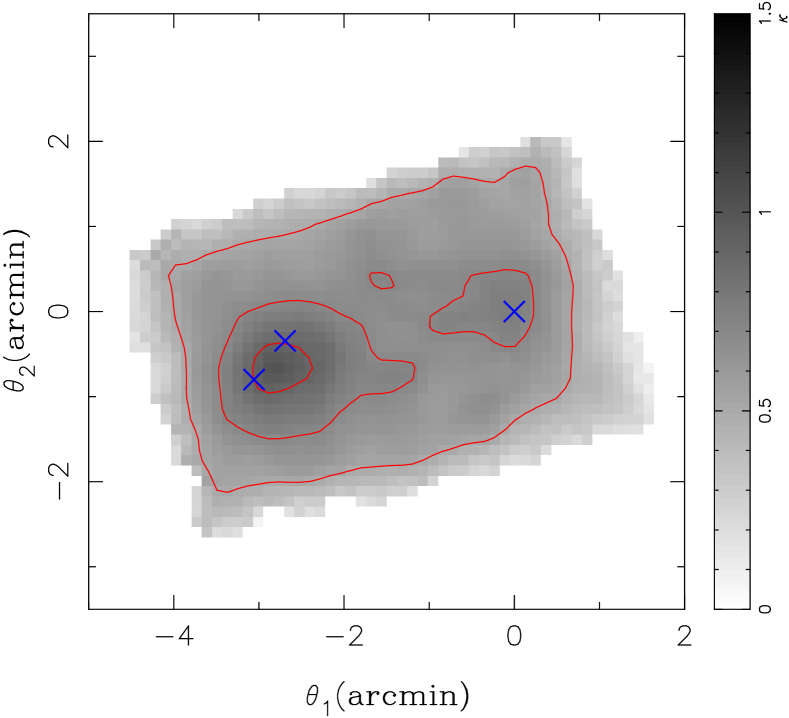
We also perform a reconstruction using the weak lensing data only (bottom-left panel of Fig. 6). From only weak lensing, we clearly detect both the main and sub clusters, but are unable to resolve individual substructures within each with high significance. This failure can in part be attributed to the limited field size used here in contrast to Clowe et al. (2006a) (our method at present does not allow us to use larger fields for the reconstruction, adaptive grid methods need to be employed then). In addition, the mass estimates from weak lensing reconstruction are unreliable (due to the the mass-sheet degeneracy); the resulting potential does not reproduce any of the multiply imaged systems observed. Traditionally, to overcome the problem of the mass-sheet degeneracy and measure the mass from the weak lensing mass reconstruction, one assumes a vanishing surface mass density at the edge of the field or adopts parametrized model fitting. The former is not applicable here because the field used is too small. The latter will yield reliable mass estimates if the assumed profile is correct, but it is difficult to guess the appropriate model for such a morphologically disturbed cluster. Combining strong and weak lensing helps us to break this degeneracy. However, the lack of counter arc candidates and redshifts of multiply imaged systems limits our ability to provide even stronger constraints on the mass distribution.
The errors on mass estimates quoted throughout the paper are obtained by summing in quadrature the errors obtained from the reconstructions using bootstrapping of the weak lensing catalogs and removing individual strong lens systems. In addition, we estimate and add systematic uncertainties resulting from differences in the reconstruction when using different initial models (as explained below). In principle, we should incorporate all of these effects simultaneously in the reconstructions, however this is too computational intensive and beyond the scope of this analysis.
5.1. Initial conditions
Methods involving strong lensing mass reconstruction with many multiple imaged systems are subject to degeneracies in parameter space. It is difficult to search the parameter space because the function has many local extrema. In our case, there are pronounced, narrow secondary minima where individual systems are reconstructed well by the model (and the others less so) and high “walls” in space where images happen to form close to the corresponding critical curves. Because weak lensing data are noisy, additional, though less pronounced, minima in are created. Given that our reconstruction method does not guarantee that we find a global minimum, in principle we would need to check the whole parameter space. This search is unfeasible with any available algorithms, given that the number of parameters (i.e., pixels in the mass map) is .
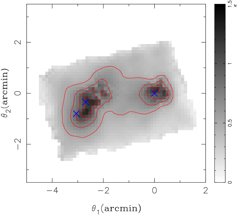
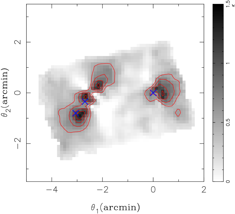
Instead, we opt to investigate the use of many initial models. We try both extremes; i.e. models that are clearly in disagreement with the data (zero initial conditions, single mass peak centered on the position of the gas) and models that use alternative methods to reconstruct the data (two-NIE model, two-NIE plus cluster members model from strong lensing modeling, weak lensing mass model from Clowe et al. 2006a). Although the details of the reconstruction depend on the initial conditions (as can be seen from comparing all but bottom-right -maps in Fig. 6), the main features (SE-NW elongation of the main cluster, two mass peaks close to the main cluster cDs, an elongation in the mass map toward the gas peak, E-W elongation of the subcluster) are independent of the particular initial model we use.
The resulting contribution of the weak lensing data remains the same for all sets of initial conditions ( for data points). The strong lensing contribution is lowest when the two component NIE model is used () and highest when the zero model initial conditions () are used. Although the absolute values of the have little meaning (i.e. one can change the regularization parameter to obtain a lower value for because the weak lensing data is noisy), the relative values tell us which resulting reconstruction is indeed a better fit to the data (as the same regularization parameters are used in all cases and it is the fit to the high signal to noise strong lensing data that improves).
We estimate the systematic uncertainty on our mass estimates by calculating the maximum difference in the resulting mass estimates when using different initial models. We exclude the zero model in this calculation as it does not predict the strong lensing data reliably. The resulting -map (see bottom-left panel in Fig. 6) for this model is suppressed where only weak lensing data are available (due to the mass-sheet degeneracy) and produce steep gradients close to arc A and a lower overall mass. However, other features in the reconstruction (positions and shapes of the mass peaks for the main and the sub-cluster) remain unchanged. In all cases, the resulting mass peaks “move” away from the initial guess; showing that the regularization is sufficiently flexible to reproduce the features in the data. Therefore, we are confident that our results are not biased as a result of the particular choices of regularization and are independent of the initial conditions to the extent presented in Fig. 6.
5.2. Strong-lens system identification and redshifts
Finally, the mass measurements presented above depend on the reliability of the redshifts and identification used for strong lensing reconstruction. These (except for system A) are not secure and depend upon the model used in Sect. 2.1. In particular, the redshifts of the systems around the subcomponents (and consequently the measurements of its mass) can change because the subcomponent mass reconstruction does not depend strongly on the modeling around the main component (where the arc with the known redshift is located).
The parametrized model used in Sect. 2.1 to estimate the redshifts of the strong lensing systems likely deviates from the truth model. We tested the dependence of the assumed redshifts by performing 100 reconstructions in which we modified all of the strong lensing system redshifts except for system A. For each reconstruction these uncertain redshifts were changed by assuming a Gaussian scatter with and requiring that all sources lie behind the cluster. The resulting mass and position errors were smaller (by a factor of 2) than the ones quoted throughout the paper, and the mass and position measurements were unbiased (as expected from such an analysis). The mass measurements would change, however, if we systematically increase (decrease) the redshifts of all the systems. For example, if we decrease the redshifts of the subcluster systems such that the lowest redshift system of the subcluster (G) is at (and scale the others accordingly), then the mass increases by a factor of . If we instead increase all the redshifts, pushing the highest redshift system (I) to ), then the mass of the subcluster will decrease by . Note however that these are just estimates, since the redshift estimates of the weak lensing sources also plays a role, and the changes will therefore be even smaller.
As a further test, we also perform 10 reconstructions where we remove one strong lens system at a time from the analysis. In Fig. 7 we show the two that differ the most from the reconstruction that uses all the strong lensing systems. When we remove system I from the reconstruction (right panel in Fig. 7) the double peaked structure of the subcluster disappears, while the east-west elongation remains. For the main cluster we see the largest deviations from the original map when we remove system D from the reconstruction (left panel in Fig. 7). However, these results do not mean that these structures are not real, rather they illustrate some possible systematics when dealing with sparse strong lensing data. We are confident that system D is indeed multiply imaged, and images I2-I3, at least, are also probably multiply imaged.
These tests demonstrate that even though the strong lensing system identification and their redshift determinations are important to the details of the reconstruction, the errors arising from misidentifications/redshift misestimation are within those quoted in the previous section.
5.3. Predictive power of the model
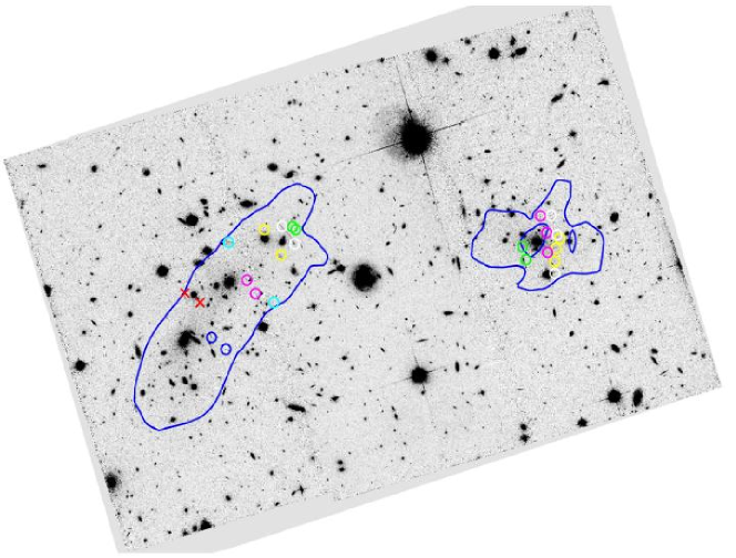
The predicted redshifts and strong lensing system identification can be tested using spectroscopy. We are planning just such a survey and will therefore be able to test the fidelity of our model in the future. In addition, using Spitzer IRAC data we identify a candidate high redshift object. While bright in all IRAC bands, the faintness of this galaxy in optical and near infrared bands indicates that it could lie at . It has two components and our predicted critical curve for this redshift (indistinguishable from the critical curve) is exactly where it should be if indeed these sources are merging images of the same source; they are denoted with crosses and plotted together with the critical curve in Fig. 8. Furthermore, we identify a candidate counter image with similar colors in the IRAC data just outside the critical curve. All three need to be further analyzed and confirmed (using spectroscopy and/or NIR data) before we include them in the modeling.
We also identify possible counter-images for systems B, J, H, and I as predicted from our model, they are indicated in Fig. 9. If these and high-redshift candidate are confirmed, the predictive power of our model would further indicate that the strong lensing data we use is reliable enough for this work.
| Main (gas peak) | 2.0 0.2 | 10.8 0.6 | 0.19 0.03 | |
| Main (S cD) | 125 (0.47) 250 (0.59) | 1.4 0.1 | 16.3 0.9 | 0.09 0.01 |
| Sub (gas peak) | 0.42 0.04 | 2.1 0.2 | 0.20 0.06 | |
| Sub (BCG) | 80 (0.31) 80 (0.31) | 0.18 0.02 | 4.3 0.2 | 0.04 0.01 |
| ACS field | 1300 (4.9) 830 (3.2) | 13 1 | 91 10 | 0.14 0.03 |
6. Conclusions and future work
Massive and interacting clusters, while quite rare, are remarkably well-suited to addressing outstanding issues in both galaxy evolution and fundamental physics. However, in order to study the mass distribution, methods relying on hydrostatic (X-rays) or dynamical equilibrium are ill-suited for such systems.
We have applied a mass reconstruction method based on strong and weak gravitational lensing to the cluster 1E065756. We use deep, high resolution optical data to identify objects belonging to the same multiple-image systems. The same data are used to obtain weak lensing catalogs allowing us to obtain a strong+weak lensing mass map of the cluster core. Our main conclusions are the following:
-
1.
Using the combined strong and weak lensing mass reconstruction we derive a high-resolution, absolutely calibrated mass map; we get projected, enclosed mass around the main and around the subcluster.
- 2.
-
3.
The majority of the mass is spatially coincident with the galaxies, which implies that the cluster mass must be dominated by a relatively collisionless form of dark matter. The high resolution data allow us to significantly detect the shapes of both the main mass component and the subcluster with no prior assumptions on their positions or profiles.
We show that the cluster 1E065756 is a very efficient strong lens; the area enclosed within the critical curve for highest redshift sources is comparable to that of A1689 Broadhurst et al. (2005). Consequently, we plan to conduct a pencil beam survey for high-redshift () objects. At present this is not possible, because we lack both reliable redshift information for the 1E065756 multiple image systems, and multi-color high-resolution imaging data in the main cluster region. The latter is needed to identify counter images for the strong lens systems, and so improve the reliability of the mass map to the south-east of the main cluster. Once these data are obtained (HST Cycle 15), we will improve our methodology to include an adaptive grid approach, which will greatly improve the constraints on the location of critical curves for these high-redshift sources.
The prospects for such a search are however very promising, as we already have two strong candidate high redshift objects. One is the red arc B, which is constrained to lie at based upon the redshift of arc A and detection in F814W. The other (see Fig. 8) is Spitzer IRAC-selected with a likely redshift of . Using this cluster as a gravitational telescope will therefore allow us to study galaxy properties near the epoch of reionization.
The high resolution mass map of this cluster, in addition to enabling the high-z galaxy search, will be valuable for several other ongoing science programs. Most significantly, we are currently running simulations to reconstruct the dynamical history of the cluster merger, and provide an independent constraint on the dark matter self-interaction cross-section. The relative masses of the main and the subcluster, and the central mass distribution, two critical parameters for the simulations, were the limiting source of uncertainty prior to this work.
References
- Barrena et al. (2002) Barrena, R., Biviano, A., Ramella, M., Falco, E. E., & Seitz, S. 2002, A&A, 386, 816
- Bartelmann & Schneider (2001) Bartelmann, M. & Schneider, P. 2001, Phys. Rep., 340, 291
- Bertin & Arnouts (1996) Bertin, E. & Arnouts, S. 1996, A&AS, 117, 393
- Bradač et al. (2005a) Bradač, M., Erben, T., Schneider, P., Hildebrandt, H., Lombardi, M., Schirmer, M., Schindler, S., & Miralles, J.-M. 2005a, A&A, 437, 49
- Bradač et al. (2004) Bradač, M., Lombardi, M., & Schneider, P. 2004, A&A, 424, 13
- Bradač et al. (2005b) Bradač, M., Schneider, P., Lombardi, M., & Erben, T. 2005b, A&A, 437, 39
- Brainerd et al. (1996) Brainerd, T. G., Blandford, R. D., & Smail, I. 1996, ApJ, 466, 623
- Broadhurst et al. (2005) Broadhurst, T., Benítez, N., Coe, D., Sharon, K., Zekser, K., White, R., Ford, H., et al. 2005, ApJ, 621, 53
- Clowe et al. (2006a) Clowe, D., Bradac, M., Gonzalez, A., Markevitch, M., Randall, S., Jones, C., & Zaritsky, D. 2006a, Accepted ApJL
- Clowe et al. (2004) Clowe, D., Gonzalez, A., & Markevitch, M. 2004, ApJ, 604, 596
- Clowe et al. (2006b) Clowe, D., Schneider, P., Aragón-Salamanca, A., Bremer, M., de Lucia, G., Halliday, C., Jablonka, P., Milvang-Jensen, B., Pelló, R., Poggianti, B., Rudnick, G., Saglia, R., Simard, L., White, S., & Zaritsky, D. 2006b, A&A, 451, 395
- Clowe et al. (2006c) Clowe, D. et al. 2006c, in preparation
- Fontana et al. (1999) Fontana, A., D’Odorico, S., Fosbury, R., Giallongo, E., Hook, R., Poli, F., Renzini, A., et al. 1999, A&A, 343, L19
- Gomez et al. (2004) Gomez, P., Romer, A. K., Peterson, J. B., Chase, W., Runyan, M., Holzapfel, W., Kuo, C. L., et al. 2004, in AIP Conf. Proc. 703: Plasmas in the Laboratory and in the Universe: New Insights and New Challenges, 361–366
- Hayashi & White (2006) Hayashi, E. & White, S. D. M. 2006, ArXiv Astrophysics e-prints
- Heymans et al. (2005) Heymans, C., Brown, M. L., Barden, M., Caldwell, J. A. R., Jahnke, K., Peng, C. Y., Rix, H.-W., Taylor, A., Beckwith, S. V. W., Bell, E. F., Borch, A., Häußler, B., Jogee, S., McIntosh, D. H., Meisenheimer, K., Sánchez, S. F., Somerville, R., Wisotzki, L., & Wolf, C. 2005, MNRAS, 361, 160
- Heymans et al. (2006) Heymans, C., Van Waerbeke, L., Bacon, D., Berge, J., Bernstein, G., Bertin, E., Bridle, S., Brown, M. L., Clowe, D., Dahle, H., Erben, T., Gray, M., Hetterscheidt, M., Hoekstra, H., Hudelot, P., Jarvis, M., Kuijken, K., Margoniner, V., Massey, R., Mellier, Y., Nakajima, R., Refregier, A., Rhodes, J., Schrabback, T., & Wittman, D. 2006, MNRAS, 368, 1323
- Jee et al. (2006) Jee, M. J., White, R. L., Ford, H. C., Illingworth, G. D., Blakeslee, J. P., Holden, B., & Mei, S. 2006, ApJ, 642, 720
- Kaiser et al. (1995) Kaiser, N., Squires, G., & Broadhurst, T. 1995, ApJ, 449, 460
- Keeton & Kochanek (1998) Keeton, C. & Kochanek, C. 1998, ApJ, 495, 157
- Kneib et al. (1996) Kneib, J.-P., Ellis, R. S., Smail, I., Couch, W. J., & Sharples, R. M. 1996, ApJ, 471, 643
- Kochanek (2004) Kochanek, C. S. 2004, astro-ph/0407232
- Koekemoer et al. (2002) Koekemoer, A. M., Fruchter, A. S., Hook, R. N., & Hack, W. 2002, in The 2002 HST Calibration Workshop, Baltimore, MD, 2002., p.339, 339
- Lupton et al. (2004) Lupton, R., Blanton, M. R., Fekete, G., Hogg, D. W., O’Mullane, W., Szalay, A., & Wherry, N. 2004, PASP, 116, 133
- Markevitch et al. (2004) Markevitch, M., Gonzalez, A. H., Clowe, D., Vikhlinin, A., Forman, W., Jones, C., Murray, S., & Tucker, W. 2004, ApJ, 606, 819
- Markevitch et al. (2002) Markevitch, M., Gonzalez, A. H., David, L., Vikhlinin, A., Murray, S., Forman, W., Jones, C., & Tucker, W. 2002, ApJ, 567, L27
- Markevitch et al. (2006) Markevitch, M. et al. 2006, in preparation
- Mehlert et al. (2001) Mehlert, D., Seitz, S., Saglia, R. P., Appenzeller, I., Bender, R., Fricke, K. J., Hoffmann, T. L., et al. 2001, A&A, 379, 96
- Randall et al. (2006) Randall, S. et al. 2006, in preparation
- Springel et al. (2001) Springel, V., White, S. D. M., Tormen, G., & Kauffmann, G. 2001, MNRAS, 328, 726
- Tucker et al. (1995) Tucker, W. H., Tananbaum, H., & Remillard, R. A. 1995, ApJ, 444, 532