A search for anisotropy in the arrival directions of ultra high energy cosmic rays recorded at the Pierre Auger Observatory

Abstract

Observations of cosmic ray arrival directions made with the Pierre Auger Observatory have previously provided evidence of anisotropy at the 99$\%$ CL using the correlation of ultra high energy cosmic rays (UHECRs) with objects drawn from the Véron-Cetty Véron catalog. In this paper we report on the use of three catalog independent methods to search for anisotropy. The 2pt–L, 2pt+ and 3pt methods, each giving a different measure of self-clustering in arrival directions, were tested on mock cosmic ray data sets to study the impacts of sample size and magnetic smearing on their results, accounting for both angular and energy resolutions. If the sources of UHECRs follow the same large scale structure as ordinary galaxies in the local Universe and if UHECRs are deflected no more than a few degrees, a study of mock maps suggests that these three methods can efficiently respond to the resulting anisotropy with a $P$-value = $1.0\%$ or smaller with data sets as few as 100 events. Using data taken from January 1, 2004 to July 31, 2010 we examined the 20, 30, …, 110 highest energy events with a corresponding minimum energy threshold of about 49.3 EeV. The minimum $P$-values found were $13.5\%$ using the 2pt-L method, $1.0\%$ using the 2pt+ method and $1.1\%$ using the 3pt method for the highest 100 energy events. In view of the multiple (correlated) scans performed on the data set, these catalog-independent methods do not yield strong evidence of anisotropy in the highest energy cosmic rays.

1 Introduction

It is almost 50 years since cosmic rays with energies of the order of 100 EeV (1 EeV$\equiv 10^{18}$ eV) were first reported [1]. Soon after the initial observation of such cosmic rays it was realized by Greisen [2], Zatsepin and Kuz’min [3] that their interactions with the cosmic microwave background would result in energy loss that would limit the distance which they could travel. This would suppress the particle flux and result in a steepening of the energy spectrum. If the observed flux suppression [4, 5] is due to this mechanism, it is likely that the cosmic rays with energies in excess of $\simeq 50~{}$EeV could be anisotropic as they would originate in the local Universe. Several searches for anisotropy in the arrival directions of UHECRs have been performed in the past, either aimed at correlating arrival directions with astrophysical objects [6, 7] or searching for anisotropic arrival directions [8, 9, 10, 11]. No positive observations have been confirmed by subsequent experiments [12, 13, 14, 15].

In 2007, the Pierre Auger Observatory [16] provided evidence for anisotropy at the 99% CL (Confidence Level) by examining the correlation of UHECR ($\geq 56~{}$EeV) with nearby objects drawn from the Véron-Cetty Véron (VCV) catalog [17]. The correlation at a predefined 99% CL was established with new data after studies of an initial 15 event-set defined a likely increase in the UHECR flux in circles of $\simeq 3^{\circ}$ radius around Active Galactic Nuclei (AGNs) in the VCV catalog with redshift $\leq 0.018$ [18, 19]. An updated measurement of this correlation has recently been given, showing a reduced fraction of correlating events when compared with the first report [20].

The determination of anisotropies in the UHECR sky distribution based on cross-correlations with catalogs may not constitute an ideal tool in the case of large magnetic deflections and/or transient sources. Also, some signal dilution may occur if the catalog does not trace in a fair way the selected class of astrophysical sites, due for instance to its incompleteness. As an alternative, we report here on tests designed to answer the question of whether or not the arrival directions of UHECRs observed at the Pierre Auger Observatory are consistent with being drawn from an isotropic distribution, with no reference to extragalactic objects. The local Universe being distributed in-homogeneously and organized into clusters and superclusters, clustering of arrival directions may be expected in the case of relatively low source density. Hence, the methods used in this paper are based on searches for the self-clustering of event directions at any scale. These may thus constitute an optimal tool for detecting an anisotropy and meanwhile provide complementary information to searches for correlations between UHECR arrival directions and specific extragalactic objects.

The paper is organized in the following manner. The three methods we use in this paper, the 2pt-L, 2pt+ and 3pt methods, are explained in Section 2. In Section 3, we apply these methods to a toy model of anisotropy to address the importance of systematic uncertainties from both detector effects and unmeasured astrophysical parameters. In Section 4, we apply the three methods to an updated set of the Pierre Auger Observatory data. We draw final conclusions in Section 5.

2 Analysis Methods

At the highest energies, the steepening of the cosmic ray energy spectrum makes the current statistics so small that a measure of a statistically significant departure from isotropy is hard to establish, especially when using blind generic tests. This motivated us to develop several methods by testing their efficiency for detecting anisotropy using simulated samples of the Auger exposure with 60 data points drawn from different models of anisotropies both on large and small scales. The choice of 60 events for the mock catalogs was based on the number of events expected for an exposure of two full years of Auger above the $\approx 50$ EeV energy threshold for anisotropy. We report in this paper on self-correlation analysis, using differential approaches based on a 2pt-L function [21, 22], an extended 2pt function [23] (“2pt+”) and a 3pt function [22] (“3pt”).

2.1 The 2pt-L method

The 2-point correlation function [21] is defined as the differential distribution over angular scale of the number of observed event pairs in the data set. There are different possible implementations of statistical measures based on the 2pt function. We adopt in this work the one in [22] (named 2pt-L in the following), where the departure from isotropy is tested through a pseudo-log-likelihood as described below. The expected distribution of the 2pt-L correlation function values was built using a large number of simulated background sets drawn from an isotropic distribution accounting for the exposure of the experiment. We use angular bins of 5 degrees to histogram the angle ($\lambda$) between event pairs over a range of angular scales. The pseudo-log-likelihood is defined as $\mathcal{L}_{2pt-L}$ :

$$\mathcal{L}_{2pt-L}^{data}=\sum_{i=1}^{N_{bins}}\ln{P(n_{obs}^{i}|n_{exp}^{i})},$$ (2.1)

where $n_{obs}^{i}$ and $n_{exp}^{i}$ are the observed and expected number of event pairs in bin $i$ and $P$ the Poisson distribution. The resulting $\mathcal{L}_{2pt-L}^{data}$ is then compared to the distribution of $\mathcal{L}_{2pt-L}$ obtained from isotropic Monte-Carlo samples. The $P$-value $P_{2pt}$ for the data to come from the realization of an isotropic distribution is finally calculated as the fraction of samples whose $\mathcal{L}_{2pt-L}$ is lower than $\mathcal{L}_{2pt-L}^{data}$.

2.2 The 2pt+ method

The 2pt-L method is sensitive to clusters of different sizes, but not to the relative orientation of pairs. To pick up filamentary structures or features such as excesses of pairs aligned along some preferential directions, an enhanced version of the classic 2pt-L test was devised: the 2pt+ method [23]. In addition to the angular distance $\lambda$ between event pairs, the 2pt+ test uses two extra variables related to the orientation of each vector connecting pairs. As either one of the points in the pair can be regarded as the vector origin, the point of origin is always chosen so that the z-axis component is positive. This point is translated to the center of a sphere giving rise to the two new variables, $\cos(\theta)$ which is the cosine of the vector’s polar angle, and $\phi$, which is the vector’s azimuthal angle. It is worth noticing that, contrary to the distance $\lambda$ between event pairs, these two additional variables are not independent of the reference system in which they are calculated. All results presented hereafter have been obtained with the z-axis pointing toward the Northern pole in equatorial coordinates. Fig. 1 schematically depicts the definitions of the variables that are used in this method. The left panel shows the vector between two points on a sphere, subtending an angle $\lambda$, which we aim to describe using three independent variables. The vector between two events translated to the origin of coordinates, can be described using the following 3 variables as in the right panel of Fig. 1:

1. $\cos\lambda$, which is a measure of the length of the vector;

2. $\cos\theta$, which is the cosine of the vector’s polar angle; and

3. $\phi$, which is the vector’s azimuthal angle.

To measure the departure from isotropy, the 2pt-L distribution and the two angular distributions can be combined into one single estimator. First, in the same way as in the 2pt-L test, a binned likelihood test is applied to the $\cos{(\lambda)}$ distribution (using a number of bins such that the expected number of pairs in each bin is $n_{exp}^{i}=5$), and a $P$-value $P_{\lambda}$ is obtained as the fraction of samples whose pseudo-log-likelihood $\mathcal{L}_{\lambda}$ is lower than $\mathcal{L}_{\lambda}^{data}$. Then, making use of the $\cos{\theta}$ and $\phi$ distributions, another pseudo-log-likelihood $\mathcal{L}_{\theta,\phi}$ is defined as :

$$\mathcal{L}_{\theta,\phi}^{data}=\sum_{j,k=0}^{N_{bins},\theta\phi}\ln{P(n_{j,k}^{\theta\phi,obs},\mu)},$$ (2.2)

where $P(n_{j,k}^{\theta\phi,obs},\mu)$ is the Poisson distribution with mean $n_{j,k}^{\theta\phi,exp}=5$ and $n_{j,k}^{\theta\phi,obs}$ is the observed number of pairs in the $j^{th}k^{th}$ $(\cos\theta,\phi)$ bin. The $P$-value $p_{\theta,\phi}$ is obtained in the same way as previously. Finally, the combined $P$-value is calculated using Fisher’s method :

$$P_{combined}=P_{\lambda}p_{\theta\phi}(1-\ln P_{\lambda}p_{\theta\phi}).$$ (2.3)

However, $\mathcal{L}_{\lambda}$ and $\mathcal{L}_{\theta,\phi}$ are slightly correlated tests. Hence, $P_{combined}$ needs to be corrected for these small correlations. The final $P$-value $P_{2pt+}$ is consequently calculated by correcting $P_{combined}$ using Monte-Carlo simulations.

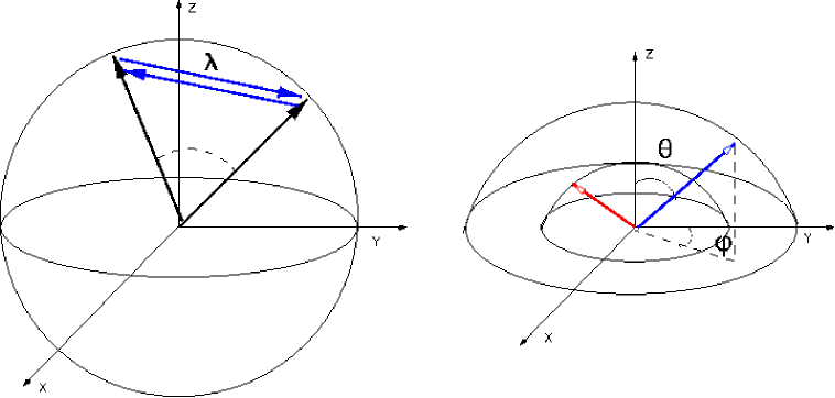
Figure 1: Schematic depiction of the variables used in the 2pt+ test. Left panel: angular distance $\lambda$ between two events. Here, the drawn sphere corresponds to the observed celestial sphere. The black vectors correspond to vectors extending from the origin (observer) to each of the two events. The blue vectors represent the two choices for the definition of the vector between events. In this work, we always use the vector with a positive $z-$component (in the case depicted here, the vector pointing from right to left). $\lambda$ is the angle subtended by the two event vectors. Right panel: angles $\theta$ and $\phi$. Here, the vectors between events have been transported to the origin, and each of the two vectors corresponds to a different pair between events. The length of each vector depends on $\lambda$, so the radii of the two spheres drawn here quantify the angular distance between each pair of events. The angles $\theta$ and $\phi$ for one of the pairs (the one represented by the blue vector) are shown in the figure. Figure from [23].

2.3 The shape strength 3pt method

Event direction clustering can also be revealed by searching for excesses of triplets through, for instance, the use of a 3-pt correlation function. The 3pt method we use hereafter is a variation of the one presented in Ref. [24, 25], involving an eigenvector decomposition of the arrival directions of all triplets found in the data set [22] . For each cosmic ray we convert the arrival direction into a Cartesian vector $\vec{r}_{k}$=$\{r_{x},r_{y},r_{z}\}$. Then we compute an orientation matrix $T_{ij}=\frac{1}{3}\sum_{k\in triplet}\left(r_{i}r_{j}\right)_{k}$ for $i,j\in\{x,y,z\}$ from which we calculate eigenvalues ($\tau$) of each $T_{ij}$ and order them $\tau_{1}\geq\tau_{2}\geq\tau_{3}\geq{0}$ (subject to the constraint $\tau_{1}+\tau_{2}+\tau_{3}=1$). The largest eigenvalue of $\mathbf{T}$, $\tau_{1}$, results from a rotation of the triplet about the principle axis $\vec{u}_{1}$. The middle and smallest eigenvalues correspond to the major $\vec{u}_{2}$ and minor $\vec{u}_{3}$ axis respectively. The left panel of Fig. 2 shows a graphical illustration of these eigenvectors. The eigenvalues are transformed into two parameters, a “strength parameter”$\zeta$ and a “shape parameter” $\gamma$ defined as :

$$\zeta=\ln(\tau_{1}/\tau_{3}),$$ (2.4)

$$\gamma=\ln\left\{\frac{\ln(\tau_{1}/\tau_{2})}{\ln(\tau_{2}/\tau_{3})}\right\}.$$ (2.5)

As $\zeta$ increases from 0 to $\infty$ the events in the triplet become more concentrated. Generally, as $\gamma$ increases from $-\infty$ to $+\infty$ the shape of the triplet transforms from elliptical, i.e. strings, to symmetric about $\vec{u}_{1}$, i.e. point source. See the right panel of Fig. 2 for a schematic representation.

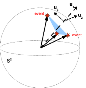
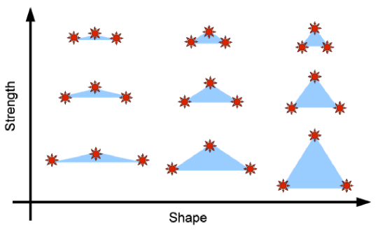
Figure 2: Left: The eigenvectors of a triplet of events on the sphere ($S^{2}$) are the principle axis $\vec{u}_{1}$, the major axis $\vec{u}_{2}$ (pointing into the page) and the minor axis $\vec{u}_{3}$. The eigenvalues of these vectors are used to compute this triplet’s shape and strength. Right: An intuitive interpretation of the shape and strength parameters. As the strength parameter $\zeta$ increases from $0$ to $\infty$, the events become more concentrated. As the shape parameter $\gamma$ increases form $-\infty$ to $+\infty$, the events become more rotationally symmetric or less elongated. Figures from [22].

After all triplets are transformed into the parameters $\gamma$ and $\zeta$, they are binned in a 2-d histogram. As $\zeta$ increases from 0 to $\infty$, the events in the triplets become more concentrated, while, as $\gamma$ increases from $-\infty$ to $+\infty$, the triplets transform from elongated elliptical to symmetric shape. This distribution is then compared against the one obtained from all triplets on a large number of Monte-Carlo isotropic samples. The departure of the data from isotropy is then measured in the same way as before, through a pseudo-log-likelihood $\mathcal{L}_{3pt}$ where we use the Poisson distribution to evaluate in each bin of ($\zeta,\gamma$) the probability of observing $n_{obs}^{i}$ counts while the expected number of counts obtained from isotropic samples is $n_{exp}^{i}$.

3 Application of methods to Monte-Carlo data sets

The use of mock data sets built from the large scale structure of the Universe provides a useful tool to study the sensitivity of the three methods. The toy model we choose here allows us to probe the efficiency of the methods by varying several parameters such as the total number of events, the dilution of the signal with the addition of isotropic events, the source density, and the external smearing applied to mock data set arrival directions. This external smearing (non angular resolution) reflects the unknown deflections imposed by the intervening galactic and extragalactic magnetic fields upon charged particles whose mass composition remains uncertain above $\simeq$ 40 EeV. In addition, the impact of both the angular and energy resolutions of the experiment can be probed in individual realizations of the underlying toy model.

Throughout this section, we present the performances of the three methods in terms of the power at different threshold values. The threshold $\alpha$ - or type-I error rate - is the fraction of isotropic simulations in which the null hypothesis is wrongly rejected (i.e., the test gives evidence of anisotropy when there is no anisotropy). The power is $1-\beta$ where $\beta$ is the type-II error rate which is the fraction of simulations of anisotropy in which the test result does not reject the null hypothesis of isotropy.

3.1 The toy model

The model we chose to use is the one described in Ref. [26]. It relies on (realistic large scale structure) mock-catalogs of cosmic rays above 40 EeV, for a pure proton composition, assuming their sources are a random subset of ordinary galaxies in a simulated volume-limited survey, for various choices of source density which are thought to be in the relevant range : $10^{-3.5}$, $10^{-4.0}$ and $10^{-4.5}$ Mpc^-3. The differential spectrum at the source is taken to be $E^{-2.3}$, and energy losses through redshift, photo-pion production and pair production are included. To get a realistic treatment of UHECRs in the GZK transition region (above  50 EeV), a realistic volume-limited source galaxy catalog is needed to a much larger depth than is available in present-day ”all sky” galaxy surveys. In particular, the galaxy catalog from which the source catalog is built must be much denser than $10^{-3.5}$ Mpc^-3 to simulate a source catalog with that particular density value. Therefore, Ref.  [26] made use of the ”Las Damas” mock galaxy catalogs [27] which were created using $\Lambda$CDM simulations with parameters that are tuned to agree with Sloan Digital Sky Survey observations.

The strength and distribution of intervening magnetic fields remain poorly known, and large deflections may be observed even for protons [28]. In the absence of a detailed knowledge of both magnetic fields and mass composition of CRs above 40 EeV, we smear out each arrival direction by adopting a Gaussian probability density function with a characteristic scale ranging from 1^∘ to 8^∘. This angle is treated as a free model parameter, and each mock data set has a fixed smearing angle.

The use of a pure proton composition in this toy model is just aimed at providing a realistic shortening of the CR horizon in the simulations through the GZK effect. Similar behavior would be obtained in the case of heavier nuclei, through photo-disintegration processes. The mock data sets produced with large smearing angles are intended to probe the lowering of the efficiencies of the methods for situations in which the magnetic deflections get larger, necessarily the case if the composition gets heavier. Smearing angles larger than 8^∘ would yield almost isotropic maps, lowering to a large extent the detection power of the methods.

Examples of sky maps produced from this toy model are shown in Fig. 3, 4. In Fig. 3, a high source density of $10^{-3.5}$ Mpc^-3 is used with an intermediate smearing angle of 5^∘. When the 3pt method is applied to the 60 highest energy events from these arrival directions, a $P$-value $P_{3pt}\approx$ 0.5 is found and the 2pt+ method yelds the same value. On the other hand, in Fig. 4, a smaller source density is used, still with an intermediate smearing angle of 5^∘. Much more clustering can be observed. When the 3pt method is applied to the 60 highest energy events, a $P$-value $P_{3pt}\approx$ 0.003 is found and the 2pt+ value is $P_{2pt+}\approx 0.004$.

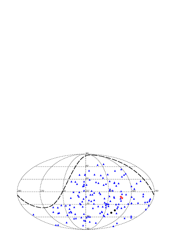
Figure 3: This map shows the Monte Carlo generated arrival directions of cosmic rays from a map with a $10^{-3.5}$ Mpc^-3 source density and a 5^∘ angular smearing for 150 events. This is an example of map which is consistent with isotropy. The upward triangles (in blue) are single events that come from different sources. The other symbols represent sets of events that came from the same source.

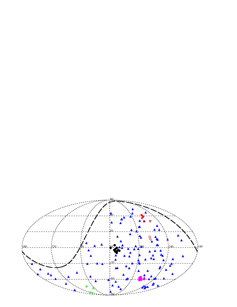
Figure 4: This map shows the Monte Carlo generated arrival directions of cosmic rays from a map with an $10^{-4.5}$ Mpc^-3 source density and a 5^∘ angular smearing for 150 events. This is an example of a map which is not consistent with isotropy. The upward triangles (in blue) are single events that come from different sources. The other symbols represent sets of events that came from the same source.

3.2 Application of methods to Monte-Carlo data sets

In the toy model, the shortening of the horizon at ultra high energies (UHE) implies that CRs must come from relatively close sources ($\lesssim$ 250 Mpc) above UHE thresholds. When the energy threshold is reduced, the CR horizon is increased and the distribution of sources becomes isotropic. This GZK effect induces a signal dilution as the energy threshold is lowered, implying a loss of sensitivity of the three methods for detecting anisotropy [23, 22]. Through this mechanism, the effects of dilution and sample size are interconnected. We study below the efficiencies of the methods by varying the sample size, the source density, and the external smearing. The powers of the methods applied to mock data sets built with a large external smearing and a high source density of $10^{-3.5}~{}$Mpc^-3 are expected to be low, while an anisotropy in mock data sets built with a low external smearing and a low source density of $10^{-4.5}~{}$Mpc^-3 is expected to be observed with much higher powers.

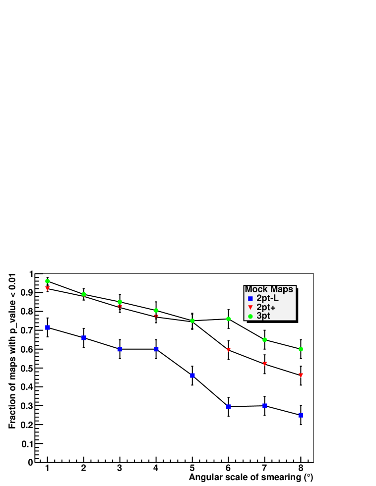
Figure 5: Powers of the 2pt-L, 2pt+ and 3pt methods for a threshold value $\alpha=1\%$. The mock sets shown are for 60 events drawn from maps with a source density of $10^{-4.5}$ Mpc^-3. The results are shown for external angular smearings ranging from 1 to 8^∘. The 2pt+ and 3pt methods perform better than the 2pt-L method and all three methods have decreased performances for larger angular smearing.

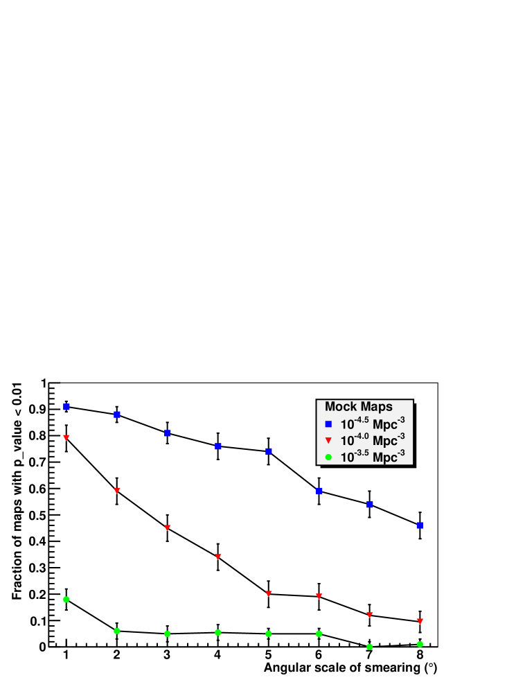
Figure 6: Power of the 2pt+ method for a threshold value $\alpha=1\%$, for different source density values. The mock data sets shown are for 60 events drawn from maps with source densities of $10^{-3.5}$, $10^{-4.0}$ and $10^{-4.5}$ Mpc^-3. The results are shown for external angular smearings ranging from 1 to 8^∘. The 2pt+ method is clearly more efficient at smaller densities (the same behavior is also observed with the other two methods).

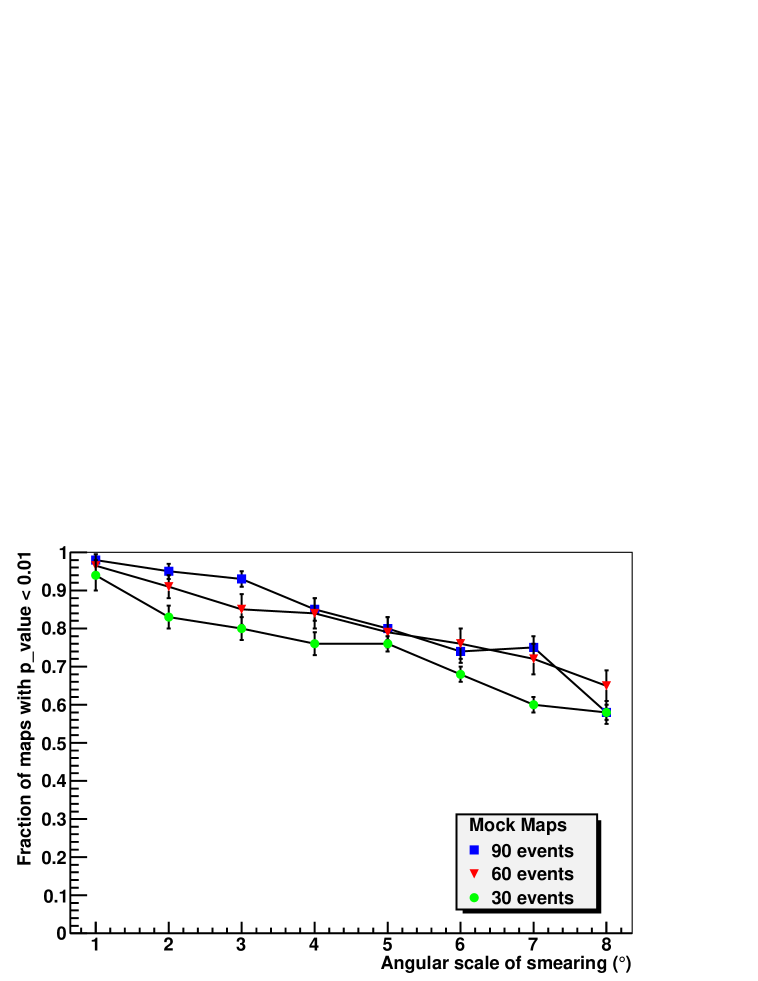
Figure 7: Power of the 3pt method for a threshold value $\alpha=1\%$, for different numbers of events (30, 60, and 90) and for a source density of $10^{-4.5}$ Mpc^-3. The results are shown for external angular smearing ranging from 1 to 8^∘. The energy threshold of the highest energy 30, 60 and 90 events is equivalent to about 64, 54 and 47 EeV respectively.

Finite angular and energy resolutions constitute an experimental source of signal dilution. Finite angular resolution is expected to slightly smooth out any clustered pattern, while finite energy resolution is expected to allow low energy events to leak into higher energy populations due to the combination of the steepening of the energy spectrum and of the sharp energy threshold used in the analysis. Above 40 EeV, the angular resolution, defined as the angular aperture $\theta_{0}$ around the arrival directions of CRs within which 68% of the showers are reconstructed, is as good as $\theta_{0}\simeq 0.8^{\circ}$ [29]. To probe the effect of this finite angular resolution, the arrival direction of each event from any mock data set is smeared out according to the Rayleigh distribution with parameter $\theta_{0}/1.51$, where the factor 1.51 is tuned to give the previously defined angular resolution. To model the uncorrelated energy resolution, the energy of each mock event is smeared out according to a Gaussian distribution centered around the original energy and with a R.M.S. $\sigma_{E}$ such that $\sigma_{E}/E=10\%$. This uncorrelated energy resolution value, relative to the absolute energy scale, is a fair one, accounting for both statistical and systematic uncertainties at the energies E $>$ 49 EeV reported in this paper.  [30]. Results shown below have been obtained by applying both angular and energy smearings to each mock data set.

The results of the Monte-Carlo studies are shown in Fig. 5, 6 and 7. These three figures show the powers obtained with each method as a function of the external angular smearing ranging from 1 to 8^∘. For Fig. 5, 6 and 7 error bars represent the binomial uncertainties from the Monte Carlo sampling. A general feature is the large decrease of performances for larger angular smearings. In Fig. 5, the power of the three methods applied to mock maps using the 60 highest energy events drawn from a source density of $10^{-4.5}$ Mpc^-3 is shown. The better performances of both the 2pt+ and the 3pt methods with respect to the 2pt-L method can be observed. In Fig. 6, the effect of changing the source density from $10^{-3.5}$ Mpc^-3 to $10^{-4.0}$ Mpc^-3 and to $10^{-4.5}$ Mpc^-3 is shown by means of the 2pt+ method, still using the 60 highest energy events. The 2pt+ method is clearly more efficient at smaller densities (a similar effect is observed for the 2pt-L and 3pt methods). In Fig. 7 the effect of using the 30, 60 and 90 highest energy events with a low source density of $10^{-4.5}$ Mpc^-3 is illustrated using the 3pt method. Provided that the number of events in the sky is between 30 and 90 events, it appears that there is no strong variation in the power of the 3pt method when using such a low density.

From these studies, it is apparent that searches for deviations from isotropic expectations of self-clustering at any scale, using the 2pt+ and 3pt methods, provide powerful tools to detect (with a threshold of 1%) an anisotropy induced by the shortening of the CR horizon at UHE, even when dealing with less than 100 events. Accounting for both angular and energy resolutions, in the case of source densities of the order of $10^{-4.5}$ Mpc^-3, the power of both methods is higher than 80% as long as the external smearing is less than $\simeq 3-4^{\circ}$. On the other hand, for higher external smearing and/or higher source densities, the powers rapidly decrease so that the methods may often miss a genuine signal in such conditions.

4 Application of methods to data

Number of events	E-threshold (EeV)	$P$-2pt-L	$P$-2pt+	$P$-3pt
20	75.5	0.113	0.291	0.271
30	69.8	0.257	0.059	0.782
40	65.9	0.175	0.010	0.541
50	61.8	0.428	0.045	0.232
60	57.5	0.174	0.180	0.020
70	55.8	0.455	0.125	0.154
80	53.7	0.482	0.175	0.024
90	52.3	0.269	0.013	0.019
100	51.3	0.135	0.010	0.011
110	49.3	0.239	0.083	0.075

Table 1: This table shows the $P$-value for the 2pt-L, 2pt+ and 3pt methods for the highest 20,30, …, 110 energy events. The energy threshold is the energy of the lowest energy event in the sample. As a consequence of these sets being cumulative, the sets are correlated. Note that none of the data sets has a $P$-value smaller than $1\%$.

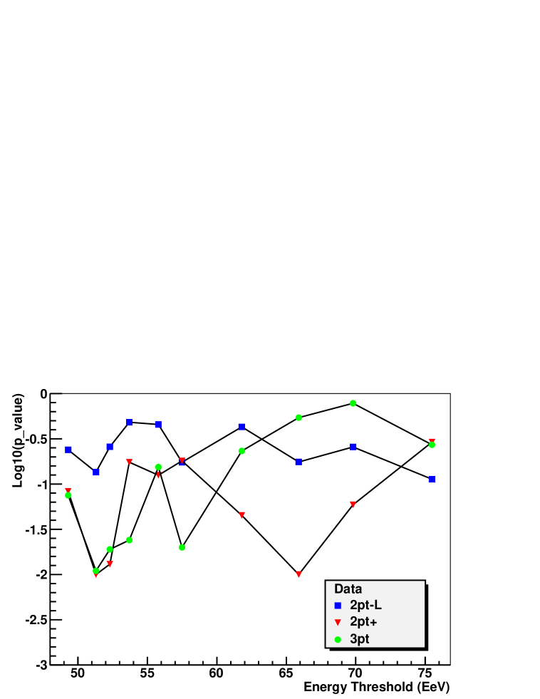
Figure 8: This shows the $P$-values of the Auger data for the 2pt-L, 2pt+ and 3pt methods. The minimum in $P$-value is at 100 events for the 2pt+ and 3pt methods and corresponds to an energy of about 51 EeV.

The data set analyzed here consists of events recorded by the surface detector array of the Pierre Auger Observatory from 1 January 2004 to 31 July 2010. During this time, the size of the Observatory increased from 154 to 1660 surface detector stations. In this analysis, we consider events with reconstructed zenith angles smaller than 60^∘, satisfying fiducial cuts requiring that at least five active stations surround the station with the highest signal, and that the reconstructed shower core is inside a triangle of active detectors when the event was recorded. At UHE, these requirements ensure both a good quality of event reconstruction and a robust estimation of the exposure of the surface detector array, which amounts to 23,344 km² sr yr for the time period used in this analysis. This exposure is 2.6 times larger than that used in Ref. [18].

The results of the three methods applied to the data from the 20 highest energy events to the highest 110 are presented in Tab. 1 and shown in Fig. 8. The strongest deviation from isotropic expectations is found at 100 events, corresponding to an energy threshold of $\simeq$ 51 EeV. The minimum $P$-values are $13.5\%$ using the 2pt-L method, $1.0\%$ using the 2pt+ method, and $1.1\%$ using the 3pt method. In view of the multiple scans performed, these tests do not provide strong evidence of anisotropy.

In case there is a true weak anisotropy in the data, the common minimum reached by the two more powerful methods (3pt and 2pt+) around $E_{threshold}\approx 51$ EeV could indicate the onset of this anisotropy, while the less powerful method (2pt-L) would not have detected it. For higher energy thresholds the number of events decrease and the power of the methods diminish as expected. If there is no weak anisotropy in the data, the Fig. 8 shows only random values of $P_{value}$ for all three methods and the common minimum mentioned before would be only a coincidence.

In our recent update on the correlation within 3.1^∘ of UHECRs ($\geq 56~{}$EeV) with nearby objects drawn from the Véron-Cetty Véron (VCV) catalog, we reported a correlating fraction of $(38^{+7}_{-6})$%, compared to 21% for isotropic cosmic rays. It is worth examining whether the null result reported here is compatible with this correlating fraction or not. For this purpose, we generated mock data sets of 80 events drawn by imposing a correlating fraction of 38% and applied both the 2pt+ and the 3pt tests on each mock data set. The detection power of the 2pt+ (3pt) test was found to be 10% (20%). These are rather low efficiencies, so that results of the correlating fraction approach and the one chosen in this study are found to be compatible.

5 Conclusion

In this paper, we have searched for self-clustering in the arrival directions of UHECRs detected at the Pierre Auger Observatory, independently of any astrophysical catalog of extragalactic objects and magnetic field hypothesis. These methods have been shown, within some range of parameters such as the magnetic deflections and the source density, to be sensitive to anisotropy in data sets drawn from mock maps which account for clustering from the large scale structure of the local Universe and for energy loss from the GZK effect. When applied to the highest energy 20, 30, …, 110 Auger events, it is found that for the 100 highest energy events, corresponding to an energy threshold of $\simeq$ 51 EeV, the $P$-values of 2pt+ and 3pt methods are about $1\%$. There is no $P$-value smaller than $1\%$ in any of the 30 (correlated) scanned values. There is thus no strong evidence of clustering in the data set which was examined.

Despite of the sensitivity improvement that the 2pt+ and 3pt tests bring with respect to the 2pt-L test, they still show relatively low powers in the case of large magnetic deflections and/or relatively high source density. In such low event number scenarios, the search for self-clustering of UHECRs is most likely not the optimal tool to establish anisotropy using the blind generic tests we presented in this paper.

References

- Linsley [1963] J. Linsley, Phys. Rev. Lett. 10, (1963) 146.
- Greisen [1966] K. Greisen, Phys. Rev. Lett. 16, (1966) 748.
- Zatsepin and Kuzmin [1966] G. T. Zatsepin and V. A. Kuzmin, JETP Lett. 4, (1966) 78.
- Abbasi et al. [2008a] R. Abbasi et al. (The HiRes Collaboration), Phys. Rev. Lett. 100, (2008a), 101101, astro-ph/0703099.
- Abraham et al. [2008b] J. Abraham et al. (The Pierre Auger Collaboration), Phys. Rev. Lett. 101, (2008b) 061101, arXiv:0806.4302[astro-ph].
- Tinyakov and Tkachev [2001a] P. G. Tinyakov and I. I. Tkachev, JETP Lett. 74, (2001a) 445, astro-ph/0102476.
- Gorbunov et al. [2002] D. S. Gorbunov, P. G. Tinyakov, I. I. Tkachev, and S. V. Troitsky, Astrophys. J. 577, (2002) L93, astro-ph/0204360.
- Stanev et al. [1995] T. Stanev, P. L. Biermann, J. Lloyd-Evans, J. P. Rachen, and A. A. Watson, Phys. Rev. Lett. 75, (1995) 3056, astro-ph/9505093.
- Uchihori et al. [2000] Y. Uchihori et al., Astropart. Phys. 13, (2000) 151, astro-ph/9908193.
- Tinyakov and Tkachev [2001b] P. G. Tinyakov and I. I. Tkachev, JETP Lett. 74, (2001b) 1, astro-ph/0102101.
- Takeda et al. [1999] M. Takeda et al., Astrophys. J. 522, (1999) 225, astro-ph/9902239.
- Abbasi et al. [2008b] R. U. Abbasi et al., (The HiRes Collaboration), Astropart. Phys. 30, (2008b) 175, astro-ph/0804.0382.
- Abbasi et al. [2007] R. U. Abbasi et al. (The HiRes Collaboration), Astropart. Phys. 27, (2007) 512, astro-ph/0507663.
- Westerhoff [2004] S. Westerhoff (The HiRes Collaboration), Nucl. Phys. (Proc. Suppl.) 136C, (2004) 46, astro-ph/0408343.
- [15] R. Abbasi (The HiRes Collaboration), %‘‘A␣Search␣for␣Three␣and␣Four␣Point␣Correlation␣in␣HiRes␣Stereo␣Data,’’%****␣3pt2pt+2pt.tex␣Line␣750␣****astro-ph/0901.3740.
- Abraham et al. [2004] J. Abraham et al. (The Pierre Auger Collaboration), Nucl. Instrum. Meth. A523, (2004) 50.
- Véron-Cetty and Véron [2006] M.-P. Véron-Cetty and P. Véron, Astron. Astrophys. 455, (2006) 773.
- Abraham et al. [2007] J. Abraham et al. (The Pierre Auger Collaboration), Science 318, (2007) 938, arXiv:0711.2256[astro-ph].
- Abraham et al. [2008a] J. Abraham et al. (The Pierre Auger Collaboration), Astropart. Phys. 29, (2008a) 188, arXiv:0712.2843[astro-ph].
- Abraham et al. [2010a] J. Abraham et al. (The Pierre Auger Collaboration), Astropart. Phys. 34, (2010a) 314, arXiv:1009.1855[astro-ph.HE]
- Peebles [1980] P.J.E Peebles, The Large-Scale Structure of the Universe, Princeton University Press, (1980)
- Hague et al. [2009] J. D. Hague, B. R. Becker, M. S. Gold, and J. A. J. Matthews, J. Phys. G36, (2009) 115203, arXiv:0905.4488[astro-ph.IM].
- Ave et al. [2009] M. Ave et al., JCAP 0907, (2009) 023, arXiv:0905.2192[astro-ph.CO].
- Woodcock [1977] N. H. Woodcock, Geological Society of America Bulletin 88, (1977) 1231.
- Woodcock [1983] N. H. Woodcock, Journal of Structural Geology 5, (1983) 539.
- [26] A. Berlind, N. Busca, G. R. Farrar and J. P. Roberts, arXiv:1112.4188, 2011.
- [27] McBride et al. in preparation (2012), see http://lss.phy.vanderbilt.edu/lasdamas/ for full details.
- Ryu et al. [2008] D. Ryu, H. Kang, J. Cho, and S. Das, Science 320, (2008) 909, ArXiv:0805.2466.
- Bonifazi [2009] C. Bonifazi, for the Pierre Auger Collaboration., Nucl. Phys. B (Proc. Suppl.) 190, (2009) 20, %****␣3pt2pt+2pt.tex␣Line␣850␣****arXiv:0901.3138[astro-ph.HE]
- Pesce [2011] M. Pesce, for the Pierre Auger Collaboration., Proc. of the 32th ICRC, Beijing, China (2011), arXiv:1107.4809[astro-ph].