Correlation function of ultra-high energy… Correlation function of ultra-high energy cosmic rays favors point sources. P. G. Tinyakov and I. I. Tkachev Tinyakov, Tkachev

Correlation function of ultra-high energy cosmic rays favors point sources.

Abstract

We calculate the angular two-point correlation function of ultra-high energy cosmic rays (UHECR) observed by AGASA and Yakutsk experiments. In both data sets, there is a strong signal at highest energies, which is concentrated in the first bin of the size of the angular resolution of the experiment. For the uniform distribution of sources, the probability of a chance clustering is $4\times 10^{-6}$. Correlations are absent or not significant at larger angles. This favors the models with compact sources of UHECR.

98.70.Sa

1.

The measurements of the flux of UHECR at energies of order $10^{20}$ eV [1] provide compelling evidence of the absence of the Greisen-Zatsepin-Kuzmin (GZK) cutoff [2]. The resolution of this puzzle seems to be impossible without invoking new physics or extreme astrophysics. All models suggested so far can be classified in three groups, according to the way the GZK cutoff is avoided: i) “nearby source” ii) weak interaction with CMB iii) bump in the injection spectrum.

The possibility i) assumes that a substantial fraction of the observed UHECR comes from a relatively nearby source(s) and thus is not subject to the GZK cutoff. This idea may be realized in different ways, examples being the models of decaying superheavy dark matter [3] or models in which UHECR emitted by nearby source(s) propagate diffusively in the galactic [4] or extragalactic [5] magnetic fields. Although models of this type generically predict large-scale anisotropy [6, 5], they might still work.

In the option ii) the GZK cutoff is eliminated (or shifted to higher energies) by assuming weak or non-standard interaction of primary particles with the cosmic microwave background. This may happen, for instance, if primary particles are neutrinos [7], hypothetical light SUSY hadrons [8], or if the Lorentz invariance is violated at high energies [9]. The possibility iii) can be realized in models which involve topological defects [10] or in some models where primary particles are neutrinos [11].

Existing data hint also at another important feature of UHECR, namely, the clustering at small angles [12]. The AGASA collaboration has reported three doublets and one triplet out of 47 events with energies $E>4\times 10^{19}$ eV, with chance probability of less than 1% in the case of the isotropic distribution [13]. The world data set has also been analyzed; 6 doublets and 2 triplets out of 92 events with energies $E>4\times 10^{19}$ eV were found [14], with the chance probability less than 1%.

If not a statistical fluctuation, what does the clustering imply for models of UHECR? There are two possible situations: either clustering is due to the existence of point-like sources, or it is a result of variations in the flux of UHECR over the sky (the regions of higher flux are more likely to produce clusters of events [15]). In the first case, the models which involve the diffuse propagation of UHECR are excluded. This case also implies that there is no defocusing of UHECR in the magnetic fields during their propagation. Such defocusing occurs even in a regular (e.g., galactic) magnetic field, since different events in a cluster have different energies. Thus, one can put bounds on the charge of the primary particles. For the extra-galactic rays, knowing that primary particles are charged would imply direct bounds on the extra-galactic magnetic fields.

In the second case, the regions of higher flux may reflect higher density of sources as in the models of superheavy dark matter where they would correspond to dark matter clumps in the halo. Alternatively, they may be due to the effects of propagation such as defocusing in magnetic fields or magnetic lensing [16].

In order to determine which of these two cases fits the present experimental data better, it is not enough to know the probability to have a certain number of clusters. In this respect previous analyses [12, 13, 14] are not sufficient. One has to find the angular correlation function. This is the approach we accept in this paper.

2.

The two-point correlation function for a given set of events is defined as follows. For each event, we divide the sphere into concentric rings (bins) with fixed angular size (say, the angular resolution of the experiment). We count the number of events falling into each bin, sum over all events and divide by 2 to avoid double counting, thus obtaining the numbers $N_{i}$. We repeat the same procedure for a large number (typically $10^{5}$) of randomly generated sets and calculate the mean Monte-Carlo value $N^{\rm MC}_{i}$ and the variance $\sigma^{\rm MC}_{i}$ for each bin in a standard way. The correlation function can be defined as $f_{i}={N_{i}/N^{\rm MC}_{i}}-1.$ A deviation of $f_{i}$ from zero indicates the presence of the correlations on the angular scale corresponding to $i$-th bin.

The correlation function $f_{i}$ fluctuates. In order to see whether its deviation from zero is statistically significant, we define the ratio $r_{i}=({N_{i}-N^{\rm MC}_{i})/\sigma^{\rm MC}_{i}},$ which shows the excess in the correlation function as compared to the random distribution in the units of the variance. With enough statistics, this quantity becomes a good measure of the probability of the corresponding fluctuation.

The Monte-Carlo events are generated in the horizon reference frame with the geometrical acceptance $dn\propto\cos\theta_{z}\sin\theta_{z}d\theta_{z},$ where $\theta_{z}$ is the zenith angle. Coordinates of the events are then transformed into the equatorial frame assuming random arrival time. We restrict our analysis to the events with zenith angles $\theta_{z}<45^{\circ}$ for which the experimental resolution of arrival directions is the best [14].

If clusters at highest energies are not a statistical fluctuation, one should expect that the spectrum consists of two components, the clustered component taking over the uniform one at a certain energy. The cut at an energy at which the clustered component starts to dominate should give the most significant signal. Motivated by these arguments, we calculated the probability of chance clustering as a function of energy cut. We present here the results for the AGASA [13] and Yakutsk [17] data sets (other experiments are discussed in Section 3). For these simulations we took the bin size equal to $2.5^{\circ}$ and $4^{\circ}$ for AGASA and Yakutsk, respectively, which is the quoted (see e.g. [13, 14]) angular resolution of each experiment multiplied by $\sqrt{2}$. The results are summarized in Fig. 1, which shows the probability to reproduce or exceed the observed count in the first bin, as a function of the energy cut.

Figure 1: FIG. 1. Probability to match or exceed the observed count in the first bin as a function of energy for the random distribution of arrival directions.

AGASA curve starts at $E=4\times 10^{19}$ eV because the data at smaller energies are not yet available. Yakutsk has much lower statistics. Both curves rapidly rise to 1 in a similar way when the statistics becomes poor. They suggest that the optimum energy cut is higher than can be imposed at present statistics.

The difference between our results and those of Ref. [13] (cf. Fig. 1 of this paper and Fig. 12 of Ref. [13]) is due to two reasons. First, 10 more events with $E>4\times 10^{19}$ have been observed [18] which bring a new doublet. Second, and more important, we calculate a different probability. The difference arises when there is a triplet or higher multiplets in the data. In our approach a triplet is equivalent to 3 or 2 doublets, depending on the relative position of the events (compact or aligned), while higher multiplicity clusters effectively have larger ”weight”. In Ref. [13] the probabilities of doublets and triplets are calculated separately; the probability of doublets is defined in such a way that a triplet contributes as 3/2 of a doublet. The drawback of this method is that the probabilities of doublets and triplets are not independent, and it is not clear how to combine them. Triplets and higher multiplicity clusters are better accounted for in our method, and the probability of chance clustering which we get is lower than in Ref. [13].

Figure 2: FIG. 2. Angular correlation functions of UHECR with binning angles and cuts in energy quoted in the text.

Correlation functions calculated with the energy cuts corresponding to the lowest chance probability is shown in Fig. 2. Both AGASA and Yakutsk correlation functions have substantial excess in the first bin. The peak in AGASA curve corresponds to 6 doublets (of which 3 actually form a triplet) out of 39 events. The peak in Yakutsk curve corresponds to 8 doublets (of which 3 also come from a triplet) out of 26 events.

Since the number of events in the first bin is not large, its distribution is not well approximated by the Gaussian one, and the deviation in the units of the variance is not a good measure for the probability of fluctuations. We calculated the probability directly by counting, in the Monte-Carlo simulation, the number of occurrences with the same or larger number of events in the first bin. Probabilities in the minima are small (see Fig. 1), so we have recalculated them with $10^{6}$ Monte-Carlo sets.

As the lowest probabilities were obtained by scanning over the energy, one may argue that they have to be multiplied by the number of steps in the scan. This is not, however, correct because the results at different energy cuts are not independent: higher energy set is a subset of the lower energy one. As can be seen from Fig. 1, the chance probability for AGASA is lower than $10^{-3}$ in the whole energy range $(4-5)\times 10^{19}$ eV, regardless of the number of steps in the scan. There still may be a correction factor. To estimate it we made the following numerical experiment. For $10^{3}$ randomly generated sets of events we have performed exactly the same procedure as for the real data, i.e. scanned over energies and obtained $10^{3}$ different minimum probabilities. We found that the probability less than $10^{-2}$ occurred 27 times, while the probability less than $10^{-3}$ occurred 3 times. Thus we conclude that the correction factor is of order $3$. This factor is included in the final results which are presented in Table.1.

Table 1: Table 1

experiment	bin size	$E_{\rm min}$	chance
			probability
AGASA	$2.5^{\circ}$	$4.8\cdot 10^{19}$ eV	$3\cdot 10^{-4}$
Yakutsk	$4^{\circ}$	$2.4\cdot 10^{19}$ eV	$2\cdot 10^{-3}$

We now turn to the determination of the angular size of the sources. To this end we calculate the dependence of the probability to have the observed (or larger) number of events in the first bin on the bin size. This dependence is plotted in Fig. 3. Jumps in the curves occur when a new doublet enters the first bin. Despite fluctuations, one can see that the minimum probability corresponds roughly to $2.5^{\circ}$ and $4^{\circ}$ for AGASA and Yakutsk, respectively. These numbers coincide with the angular resolutions of the experiments, as is expected for sources with the angular size smaller than the experimental resolution. Remarkably, there are no doublets in the AGASA set with separations between $2.5^{\circ}$ and $5^{\circ}$, while for the the extended source of the uniform luminosity one would expect 4 times more events within $5^{\circ}$ as there are within $2.5^{\circ}$. Thus, we conclude that the data favor compact sources with angular size less than $2.5^{\circ}$.

If primary particles are charged, actual positions of sources differ from the measured arrival directions because of the deflection in the Galactic magnetic field (GMF). If the clustering is attributed to real sources, it should not disappear but improve when the correction for GMF is taken into account. We have simulated the effect of such correction making use of the GMF models summarized in Ref. [19]. For the charge $Z=1$ and BSS_A model the peak in the first bin does not change significantly; one cannot discriminate between this case and the case of neutral particles. The peak becomes small at $Z=2$, and disappears at larger $Z$ for all GMF models of Ref.[19].

Figure 3: FIG. 3. Probability to have observed count in the first bin as a function of the bin size. Cuts in energy correspond to minima of Fig. 1.

3.

The other two UHECR experiments, Haverah Park (HP) and Volcano Ranch (VR), do not see significant clustering [22]. With the energy cut $E>2.4\times 10^{19}$ eV and the bin size $4^{\circ}$, the HP data contain 2 doublets at 1.8 expected, while VR data contain 1 doublet at 0.1 expected with isotropic distribution. Let us estimate the combined probability of clustering in all experiments assuming independent Poisson distributions. The number of observed doublets in AGASA and Yakutsk data are 6 and 8, respectively, while 0.87 and 2.2 are expected (these “effective” expected numbers of doublets are calculated from the condition that probabilities of Table 1 are reproduced, i.e. “penalty” for the energy scan is included). Thus, 17 doublets are observed at 4.97 expected, which corresponds to the Poisson probability $2\times 10^{-5}$. If HP data are excluded, the probability becomes $1\times 10^{-6}$, while with both HP and VR data excluded the probability is $4\times 10^{-6}$.

It is extremely unlikely that the clustering observed by AGASA and Yakutsk experiments is a result of a random fluctuation in an isotropic distribution. Rather, the working hypothesis should be the existence of some number of compact sources which produce the observed multiplets. Is this hypothesis consistent with HP and VR data? For a given experiment, the expected number of clusters is determined by the total number of events [20] (see also ref.[21]); at small clustering it scales like $N_{\rm tot}^{3/2}$ [20]. Taking AGASA data as a reference (6 doublets observed, 5.4 expected from sources and 0.6 expected from chance clustering) allows to estimate the expected number of doublets in other experiments by adding the doublets expected from sources and the doublets expected from the uniform background (calculated in the Monte-Carlo simulation). The results are summarized in Table 2, together with corresponding Poisson probabilities.

Table 2: Table 2

	$N_{\rm tot}$	observed	expected	probability
AGASA	39	6	$5.4+0.6$	$-$
Yakutsk	26	8	$2.9+1.6$	0.09
HP	32	2	$4.0+1.8$	0.07
VR	10	1	$0.7+0.1$	0.55

All experiments are roughly consistent with the assumption that the number of sources is such that they produce 5.4 doublets out of 39 events in average. Note that if HP data are discarded [22], the agreement between other experiments can be made better.

According to our simulations, the mean numbers of chance doublets are 0.6 and 1.6 for AGASA and Yakutsk, respectively. Therefore, most of the clusters in AGASA and Yakutsk data are likely to be due to real sources. In Fig. 4 we plot these clusters in the Galactic coordinates (small and large circles correspond to AGASA and Yakutsk events, respectively). Positions of triplets are indicated by arrows. The set of AGASA events with $E>4\times 10^{19}$ eV and Yakutsk events with $E>2.4\times 10^{19}$ eV is a suitable choice for the search of correlations with astrophysical objects.

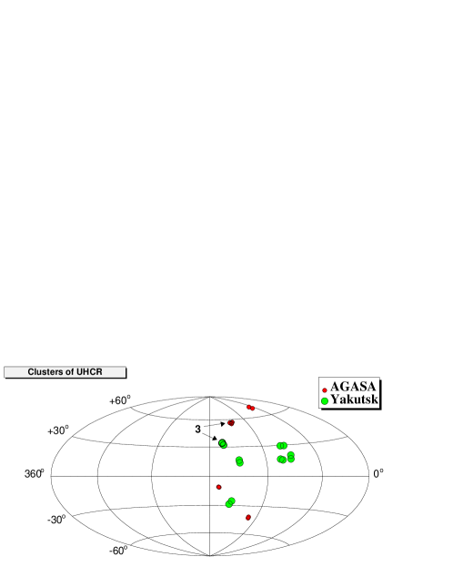
Figure 4: FIG. 4. Observed clusters in Galactic coordinates.

To summarize, the clustering of UHECR is statistically significant and favors compact sources. This places further constraints on models which can resolve the puzzle of the GZK cutoff. Those models which involve large extragalactic magnetic fields, Ref. [5], as well as models with heavy nuclei as primaries, e.g. [4], are disfavored because they assume total isotropisation of original arrival directions of UHECR. If violation of the Lorentz invariance is the solution of the GZK puzzle, and primaries are protons, our results place extremely strong limit on the extragalactic magnetic fields. Regarding the models of decaying superheavy dark matter, it is important to calculate [23] the angular correlation function predicted by these models and compare it to Fig.2 in order to see if the clumping on subgalactic scales can be responsible for the clustering of UHECR.

References

- [1] M. Takeda et al., Phys. Rev. Lett. 81, 1163 (1998); M.A. Lawrence, R.J.O. Reid and A.A. Watson, J. Phys. G: Nucl. Part. Phys., 17, 733 (1991); B.N. Afanasiev et al., Proc. Int. Symp. on Extremely High Energy Cosmic Rays: Astrophysics and Future Observatories, Ed. by Nagano, p.32 (1996).
-
[2]
K. Greisen, Phys. Rev. Lett. 16, 748 (1966);
G.T. Zatsepin and V.A. Kuzmin, Pisma Zh. Eksp. Teor. Fiz. 4, 144 (1966); - [3] V. Berezinsky, M. Kachelriess and A. Vilenkin, Phys. Rev. Lett. 79, 4302 (1997) ; V.A.Kuzmin and V.A.Rubakov, Phys. Atom. Nucl.61, 1028 (1998); V.A. Kuzmin and I.I. Tkachev, Phys. Rept. 320, 199 (1999).
- [4] P. Blasi, R.I. Epstein and A.V. Olinto, Astrophys.J.533, L123 (2000).
- [5] G.R. Farrar and T. Piran, astro-ph/0010370.
- [6] S. L. Dubovsky and P. G. Tinyakov, JETP Lett. 68, 107 (1998) [hep-ph/9802382].
- [7] T. J. Weiler, Phys. Rev. Lett. 49, 234 (1982); D. Fargion, B. Mele and A. Salis, Astrophys. J. 517, 725 (1999).
- [8] D.J.H. Chung, G. R. Farrar and E. W. Kolb, Phys. Rev. D57, 4606 (1998).
- [9] S. Coleman and S. L. Glashow, Phys. Rev. D59, 116008 (1999).
- [10] V. Berezinsky, P. Blasi, and A. Vilenkin, Phys. Rev. D58, 103515 (1998).
- [11] G. Gelmini and A. Kusenko, Phys. Rev. Lett. 84, 1378 (2000) [hep-ph/9908276].
- [12] X. Chi et al., J. Phys. G18, 539 (1992); N. N. Efimov and A. A. Mikhailov, Astropart. Phys. 2, 329 (1994).
- [13] M. Takeda et al., Astrophys. J. 522, 225 (1999).
- [14] Y. Uchihori et al., Astropart. Phys. 13, 151 (2000).
- [15] G. Medina-Tanco, astro-ph/0009336.
- [16] M. Lemoine, G. Sigl and P. Biermann, astro-ph/9903124.
- [17] Catalogue of Highest Ehergy Cosmic Rays, No. 1,2,3 World Data Center C2 for Cosmic Rays, Institute of Physical and Chemical Research, Itabashi, Tokyo, Japan.
- [18] N. Hayashida et al., astro-ph/0008102.
- [19] T. Stanev, astro-ph/9607086.
- [20] S.L. Dubovsky, P.G. Tinyakov and I.I. Tkachev, Phys. Rev. Lett. 85, 1154 (2000);
- [21] Z. Fodor and S. D. Katz, Phys. Rev. D63, 023002 (2001).
- [22] We use the data of Ref.[17]. Unpublished events were added in the analysis of Ref.[14] and more clusters were found.
- [23] S. Colombi, P. Tinyakov and I. Tkachev, in preparation.