The Geometry of (non)-Abelian adiabatic pumping

Abstract

We give a gauge description of the adiabatic charge pumping in closed systems, both in Abelian and non-Abelian processes, and by means of asymptotic Wilson loops in a suitable parameter manifold. Our geometric formulation provides new insights into this issue, and a very simple algorithm for numerical computations. Indeed, as we show first, discretized Berry–Wilczek–Zee holonomies are easy to implement. Finally, we study non-Abelian pumping in a solvable four-state model, already used in several contexts, to demonstrate the relevance of our approach.

1 Introduction

Geometry and topology play a central role in modern physics [1], obviously in advanced areas of field theories, but also in “standard” quantum mechanics. Indeed, since Berry’s seminal paper [2], an increasing number of quantum phenomena have been well understood through the mathematical apparatus of gauge theories [3, 4]. Some of the most outstanding examples are certainly to be found in quantum transport physics: Aharonov–Bohm effect, Thouless pumping, various quantum Hall effects, etc. The geometrical and topological features in question arise directly from Hilbert spaces. They are no more seen as simple vector spaces, but as bundles based on their own projective space [5] or, if the system is parameter-dependent, on a parameter manifold [2, 6].

The latter construction gives a great insight into physics of adiabatically driven quantum systems. Here, we only need to look at a single level and the initial bundle can be considerably reduced. For an $n$-fold degenerate level $(n\geqslant 1)$, a ${\rm U}(n)$ gauge structure naturally appears over parameter manifolds. The physical information is then entirely carried by Berry [2] ($n=1$) or Wilczek–Zee [7] ($n>1$) connections. Indeed, they induce parallel transports in fibres which are tantamount to the Schrödinger equation and determine the adiabatic wavefunction along parameters evolutions (up to an overall dynamical phase factor). Above all, oriented loops in parameter manifolds provide parallel transport maps called holonomies. In a standard gauge theoretic language, once given a gauge fixing, holonomies are represented by ${\rm U}(n)$ matrices known as Wilson loops. Just as representations of physical observables, these matrices transform covariantly with respect to loops’ base points. Holonomies are de facto susceptible to enclose some “elements of reality”. For example, ongoing research in quantum information tries to use them concretely for implementation of quantum logic operations [8, 9]. Besides, the gauge-covariant curvatures, naturally induced by Berry–Wilczek–Zee connections, may for their part encode some “local elements of reality”.

The non-degenerate case ($n=1$) is generic and therefore the most frequently encountered in physical literature. Notably, ${\rm U}(1)$ Wilson loops are nothing else but the celebrated Berry’s phase factor [2] accumulated by the wavefunction along a cyclic evolution. Since, in this singular Abelian case, covariance reduces to invariance, Berry’s phase is potentially measurable. As a matter of fact, it has been directly observed in a variety of interference experiments [10, 11, 12, 13, 14]. This phase has demonstrated its usefulness to interpret some concepts or phenomena [15] such as, for instance, the paradigmatic Aharonov–Bohm effect [16] whose description in terms of Berry’s phase was made by Berry himself. We can also mention the macroscopic polarization in crystalline dielectrics [17, 18, 19] expressed through Berry’s phases of Bloch states across entire Brillouin zones [20] (also called Zak’s phases), or the pumped charge in Cooper pairs pumps [21, 22, 23]. Moreover, locally, Berry’s curvature field may be taken into account to construe some physical effects. It is the case of the anomalous velocity of Bloch electrons, a correction to the usual term — coming from the band energy dispersion $\mathcal{E}(\bm{k})$ — which manifests itself when the crystal momentum $\bm{k}$ is moved by external forces [24, 25, 26, 27].

There is a close relation between Berry’s connection and current operators given by partial derivatives (or gradient) of a Hamiltonian $H$ with respect to parameter(s) [28]. This one is at the root of all the great geometrical and topological properties of systems endowed by such a current observable. Physical realizations are potentially multiple. For example, the current of Bloch electrons is proportional to $\partial_{\bm{k}}H$, while the current crossing a phase polarized Cooper pair pump is proportional to $\partial_{\varphi}H$, where $\varphi$ is the superconducting phase bias of the device. It can be shown that, when we consider a non-degenerate eigenstate of $H$, a current operator of this form splits into a usual dynamical term (coming from the energy) and a geometric correction which can be interpreted in terms of Berry’s curvature (see the example of the anomalous velocity). To the latter contribution is assigned the generic name adiabatic pumped current. In the context of the famous Thouless pumping [29], averaging the pumped current over the whole parameter manifold (a 2-torus) leads to a quantization of the charge. This stems from the topology of the line bundle over the torus, characterized by an invariant integer called first Chern number [1, 6, 28]. It is, mutatis mutandis, the same topological quantization as the Hall conductance for the integer quantum Hall effect [30, 31]. Obviously, that kind of topological invariance is highly interesting for metrological issues [32].

A. Joye et al [33] studied recently the current pumped in the degenerate non-Abelian case, too. They exhibited the differences between the Abelian and non-Abelian cases in a rigorous and somewhat abstract analytical approach. In this paper, we adopt the geometric counterpart of their work. Our aim is to give a more simple and comprehensive picture of adiabatic pumping, mainly for practical computations and later hypothetic applications (some predictions were already done within the framework of superconducting circuits [34, 35]). We reserve section 2 to a review of the basic gauge principles underlying adiabatic dynamics, and we will emphasize the central role played by Wilson loops, especially when discretized for numerical purposes. Then, section 3 is devoted to the main subject. Considering a general $n$-fold degenerate level, we will express any pumped charge in terms of some Wilson loops’ element. Contrary to what Wilson loop may seem, cyclic evolutions of the parameters are not required. The geometric difference between the two cases $n=1$ and $n>1$ will be identified. In the non-Abelian case, our holonomic formulation will allow a simple measure of “non-commutativity” of pumping cycles. Finally, in section 4, we make use of a “toy model” already encountered in non-Abelian pumping contexts [34, 33] to compare our previous results with simple analytical expressions.

2 Geometrical structure underlying quantum adiabaticity

In this section, we briefly review the peculiar geometry of quantum systems adiabatically driven by classical parameters. Broadly speaking, such parameters can be degrees of freedom having their own dynamics (e.g. nuclei positions in the Born–Oppenheimer approximation), constraints eventually tuned by experimentalists (e.g. magnetic fields and voltages in the context of quantum circuits [36]), time $t$ itself, etc. They appear as real arguments of the Hamiltonian, inducing a parameterized spectrum. If there is a total of $m$ parameters $x^{\mu}$, it is natural to represent the “parameter state” by a vector $x=(x^{1},\dots,x^{m})$ in $\mathbb{R}^{m}$. Nevertheless, for example, a periodicity of $H$ in $x^{\mu}$ can motivate us to compactify the “$\mu$-th dimension” onto $S^{1}$. Or, regarding some properties, defects may occur in a certain domain of $\mathbb{R}^{m}$ inducing “holes” in it (e.g. gauge anomalies). As a generic consequence, we are likely to use an $m$-dimensional (real) smooth parameter manifold $M$, not necessary $\mathbb{R}^{m}$. Setting $\mathcal{H}$ as the Hilbert space, we thereby construct a map $H:M\to\mathcal{L}(\mathcal{H})$ assigning to $p$ the Hamiltonian $H(p)$. An evolution of the parameters (i.e. a path in $M$) induces an evolution of the wavefunction $\Psi$ (i.e. a path in $\mathcal{H}$) via the Schrödinger equation. In the well-known adiabatic assumption, under some hypothesis, the latter obeys to a simple parallel transport rule in an “eigenspace bundle”, as reviewed below.

2.1 General settings

Let us assume that the gap hypothesis is fulfilled for an isolated eigenvalue $\mathcal{E}$ of $H$, smoothly defined everywhere on $M$. That is to say, $\mathcal{E}$ is a smooth function on $M$ and its finite multiplicity $n$ is an invariant. Let $\mathfrak{E}_{p}\simeq\mathbb{C}^{n}$ be the eigenspace corresponding to $\mathcal{E}(p)$ for each point $p$ in $M$. In the adiabatic limit, if the state is initially found in $\mathfrak{E}_{\gamma(0)}$, it is well-known [37, 38] that along a path $\gamma:\tau\mapsto\gamma(\tau)$, the wavefunction “lives” at each time $\tau$ in $\mathfrak{E}_{\gamma(\tau)}$. The whole Hilbert space being useless, one reduces the structure when “gluing” together all the spaces $\mathfrak{E}_{p}$ to yield a smooth vector bundle $\pi:\mathfrak{E}\to M$ with fibres $\pi^{-1}(p)=\mathfrak{E}_{p}$. In this bundle point of view, the adiabatic wavefunction $\Psi(\tau)\in\pi^{-1}[\gamma(\tau)]$ moves horizontally to $\gamma$. More precisely, up to an overall phase factor, $\Psi$ obeys to the BWZ parallel transport rule built as follows. Let $\{|u_{a}(p)\rangle\in\pi^{-1}(p)\}_{a=1,\dots,n}$ be a local smooth choice of orthonormal frames. Within this gauge fixing, the BWZ connection $\omega$ is locally represented by a $\mathfrak{u}(n)$-valued 1-form field $\mathcal{A}$: using a coordinate chart $x=(x^{1},\dots,x^{m})=x^{\mu}e_{\mu}$, $\mathcal{A}$ reads $A_{\mu}\,{\rm d}x^{\mu}$ with $A_{\mu\,b}^{a}:=\langle u_{a}|\partial_{\mu}u_{b}\rangle$.

We now consider a path $\gamma:\tau\mapsto\gamma(\tau)$ in $M$. In the adiabatic limit, the wavefunction is $\Psi(\tau)=e^{i\,\eta(\tau)}\,\psi(\tau)$, where

$$\eta(\tau)=-\frac{1}{\hbar}\int_{0}^{\tau}\mathcal{E}[\gamma(\tau^{\prime})]\,{\rm d}\tau^{\prime}$$

is the dynamical phase, and $\psi$ the parallel transport of $\Psi(0)=\psi(0)$ along $\gamma$. In components, if $|\psi\rangle:=\psi^{a}|u_{a}\rangle$,

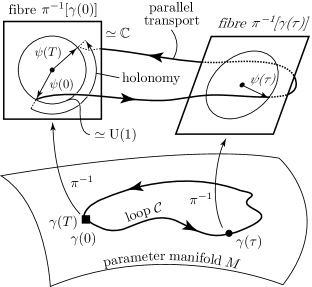
Figure 1: Illustration of the gauge structure over a parameter manifold $M$, in the Abelian case $n=1$. Parallel transport in fibres along a loop $\mathcal{C}\equiv\gamma_{T,0}$ produces a holonomy sending $\psi(0)$ to $\psi(T)$.

the parallel transport equation is

$$\dot{\psi}^{a}+A_{\mu\,b}^{a}\,\dot{x}^{\mu}\,\psi^{b}=0.$$

Its formal solution is thus

$$\psi^{a}(\tau)=W^{a}_{\;\;b}\big{[}\gamma_{\tau,0}\big{]}\,\psi^{b}(0),$$

where $\gamma_{\tau,0}\equiv\gamma|_{[0,\tau]}$ is the restriction of $\gamma$ to $[0,\tau]$, and $W$ is the Wilson operator acting on any path $\alpha$ through

$$W\big{[}\alpha\big{]}:=\mathcal{P}\,e^{-\int_{\alpha}\mathcal{A}}\in{\rm U}(n).$$ (1)

$W\big{[}\alpha\big{]}$ is commonly called a Wilson line, or, if $\alpha$ is a (based) loop, a Wilson loop [39]. Finally, one obtains the standard expression of the adiabatic wavefunction [7]:

$$|\Psi(\tau)\rangle=e^{i\eta(\tau)}W^{a}_{\;\;b}\big{[}\gamma_{\tau,0}\big{]}\,\psi^{b}(0)\,|u_{a}[p(\tau)]\rangle.$$ (2)

Let us recall how $\mathcal{A}$ and $W$ behave under a gauge transformation (i.e. a change of reference frames) generated by the smooth map $g:p\mapsto g(p)\in{\rm U}(n)$:

$$|u_{a}(p)\rangle\mapsto|\tilde{u}_{a}(p)\rangle=|u_{b}(p)\rangle\,g^{b}_{\;\;a}(p).$$ (3)

Each component $A_{\mu}$ transforms under (3) in accordance with the compatibility condition:

$$A_{\mu}(p)\mapsto\widetilde{A}_{\mu}(p)=g^{-1}(p)A_{\mu}(p)g(p)+g^{-1}(p)\,\partial_{\mu}g(p),$$ (4)

i.e. $\mathcal{A}\mapsto g^{-1}\mathcal{A}\,g+g^{-1}dg$. As for the Wilson operator, using the equality

$$A_{\mu}[\gamma(\tau)]\,\dot{x}^{\mu}(\tau)=W\big{[}\gamma_{\tau,0}\big{]}\,\partial_{\tau}W^{-1}\big{[}\gamma_{\tau,0}\big{]},$$

it is easy to check that $W\big{[}\gamma_{\tau,0}\big{]}$ transforms according to the similarity rule:

$$W\big{[}\gamma_{\tau,0}\big{]}\mapsto\widetilde{W}\big{[}\gamma_{\tau,0}\big{]}=g^{-1}\big{[}\gamma(\tau)\big{]}W\big{[}\gamma_{\tau,0}\big{]}g\big{[}\gamma(0)\big{]}.$$ (5)

Notably, if $\gamma_{T,0}$ is a loop $\mathcal{C}$, i.e. if $\gamma(T)=\gamma(0)=:p_{0}$, $W\big{[}\mathcal{C}\big{]}$ transforms covariantly with respect to its base point $p_{0}$ :

$$W\big{[}\mathcal{C}\big{]}\mapsto\widetilde{W}\big{[}\mathcal{C}\big{]}=g^{-1}(p_{0})W\big{[}\mathcal{C}\big{]}g(p_{0}).$$

Properly, in the basis $\{|u_{a}(p_{0})\rangle\}$, $W\big{[}\mathcal{C}\big{]}$ represents the parallel transport map along $\mathcal{C}$, itself an element of the BWZ holonomy group based at $p_{0}$. In particular, when $n=1$, $W\big{[}\mathcal{C}\big{]}$ reduces to Berry’s phase factor which actually depends only on the unbased loop corresponding to $\mathcal{C}$ (see figure 1). Although it is abusive, by analogy with the Abelian case, $W\big{[}\mathcal{C}\big{]}$ is often called a non-Abelian geometric phase when $n>1$. Of course, physical relevance is assigned to its eigenvalues which are gauge invariants of the parallel transport map. A good strategy consists in expressing measurable quantities as their functions (see [40] in the framework of quantum pumping). In the next section, however, it will be possible to link the pumped current to a single diagonal element of some Wilson loops.

We have not yet spoken about the BWZ curvature $\Omega$. Within a gauge fixing, it is locally represented by the 2-form field $\mathcal{F}:=d\mathcal{A}+\mathcal{A}\wedge\mathcal{A}=\frac{1}{2}\,F_{\mu\nu}\,{\rm d}x^{\mu}\wedge{\rm d}x^{\nu}$, with

$$F_{\mu\nu}=\partial_{\mu}A_{\nu}-\partial_{\nu}A_{\mu}+[A_{\mu},A_{\nu}]$$

the antisymmetric curvature tensor. It is obviously gauge covariant:

$$F_{\mu\nu}\mapsto\widetilde{F}_{\mu\nu}=g^{-1}F_{\mu\nu}\,g={\rm Ad}_{g^{-1}}\big{(}F_{\mu\nu}\big{)},$$

i.e. $\mathcal{F}\mapsto g^{-1}\mathcal{F}g$.

2.2 (Discrete) Wilson loops as fundamental ingredients of the theory

Because curvature fields and holonomies behave like observables, both are susceptible to carry some “elements of reality”, as we shall see in a while, within the framework of the pumping process. However, we will regard the latter as the most fundamental objects for two reasons.

• Any component of the curvature tensor can be expressed by means of an infinitesimal Wilson loop. Indeed, in coordinates, consider a small rectangular loop $c$ based at $x$ and oriented along the $\mu$-th then the $\nu$-th directions. Call $\ell_{\mu}$ its length in the $\mu$-th direction and $\ell_{\nu}$ in the $\nu$-th one, with $\ell_{\mu}\sim\ell_{\nu}$ (see figure 2). In the appendix, we derive the following relation:

  $$F_{\mu\nu}(x)=\frac{1}{\ell_{\mu}\ell_{\nu}}\,\Big{\{}\leavevmode\hbox{\small 1\kern-3.8pt\normalsize 1}-W\big{[}c\big{]}\Big{\}}+\Or(\ell),$$ (6)

  where the $\Or$ symbol must be here understood in a matrix norm sense, and $\ell\sim\ell_{\mu},\ell_{\nu}$ stands for the order of the “plaquette” size. The above formula can be reduced from the anti-Hermitian nature of $F_{\mu\nu}$:

  $$F_{\mu\nu}(x)=-\frac{i}{\ell_{\mu}\ell_{\nu}}\,\Im\Big{\{}W\big{[}c\big{]}\Big{\}}+\Or(\ell).$$ (7)

  

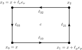
  Figure 2: The value of the curvature component $F_{\mu\nu}(x)$ is contained in Wilson loops of small oriented rectangles $c$, as defined in text. The proof given in the appendix needs a decomposition into four oriented segments $\ell_{kj}$.

• A numerical scheme can easily be implemented to compute Wilson loops arising in our context. First, note that the naive discretization of formula (1):

  $$W\big{[}\mathcal{C}\big{]}=\lim_{N\to\infty}\mathcal{P}\prod_{j=1}^{N}\Big{(}\leavevmode\hbox{\small 1\kern-3.8pt\normalsize 1}-A_{\mu}(p_{j})\Delta x^{\mu}_{j}\Big{)},$$

  with $p_{0}=p_{N}$ and $\Delta x^{\mu}_{j}:=x^{\mu}_{j}-x^{\mu}_{j-1}$, seems inapplicable since it underlies smoothness in the gauge fixing, while numerical diagonalization routines “choose” eigenvectors in a somewhat erratic manner. This difficulty is overcome by the contextual definition of $A_{\mu}$, leading to

  $$\Big{[}\leavevmode\hbox{\small 1\kern-3.8pt\normalsize 1}-A_{\mu}(p_{j})\Delta x^{\mu}_{j}\Big{]}^{a}_{\;\;b}=\langle u_{a}(p_{j})|u_{b}(p_{j-1})\rangle+\Or\big{(}N^{-2}\big{)}.$$

  After introducing the overlap matrices $S(p,q)$, whose elements are $S^{a}_{\;\;b}(p,q):=\langle u_{a}(p)|u_{b}(q)\rangle$, one obtains a formulation of great value for numerical treatments: the discrete Wilson loop

  $$W\big{[}\mathcal{C}\big{]}=\lim_{N\to\infty}\mathcal{P}\prod_{j=1}^{N}S(p_{j},p_{j-1}).$$ (8)

In the special case $n=1$, the above formula reduces to the discrete counterpart of Berry’s phase factor: it can be seen as asymptotic versions of the Pancharatnam phase factor [41] or the Bargmann invariant [42]. Covariance of (8) is easily checked. Furthermore, it allows erratic frame choices along the loop: they cancel out in pairs, whereas the geometric information is solely extracted. In fact, one has removed the rigid constraints of differentiability and continuity in frame choices, properties which in fine reveal themselves unnecessary. Building an efficient algorithm based on formula (8) is a simple task: it needs basically scalar and matrix product evaluations, and a diagonalization routine for the Hamiltonian [43]. For $n=1$, it has been already implemented in miscellaneous contexts [17, 44, 18, 45, 23]. For $n>1$, the result depends on the basis $\{|u_{a}(p_{0})\rangle\}$ chosen on input. Then, in both cases, we let the program “choose” the frame $\{|u_{a}(p)\rangle\}$ of $H(p)$ along the loop. We mainly apply formula (8) to compute $W\big{[}c\big{]}$ in (7) as

$$W\big{[}c\big{]}=\mathcal{P}\prod_{j=1}^{4}S(x_{j},x_{j-1})+\Or(\ell),$$ (9)

where $x_{0}=x_{4}=x$, $x_{1}$, $x_{2}$ and $x_{3}$ are $c$’s vertices (see figure 2).

3 Adiabatic charge pumping: a geometric viewpoint

In this section, we exhibit the geometrical significance of adiabatic charge pumping. Such a process needs a quantum system equipped with (i) a current operator $\mathcal{I}$; (ii) a Hamiltonian dependence in a controllable “pumping parameter” $\lambda\in I$, where $I$ is an interval of $\mathbb{R}$ and (iii) a suitable Hamiltonian gauge such that $\mathcal{I}$ reads $\frac{q}{\hbar}\,\partial_{\lambda}H$ [28], where $q$ is a unit of charge. Physics of pumping becomes richer in the presence of other parameters. That is why we will assume $H$ defined over an $(m+1)$-dimensional parameter manifold $M\times I$. With the current operator is naturally associated a mean transferred charge $Q$ through the relation $\dot{Q}=\langle\mathcal{I}\rangle$, that is (in units of $q$)

$$\dot{Q}(\tau):=\frac{1}{\hbar}\,\langle\Psi(\tau)|\partial_{\lambda}H[p(\tau);\lambda]|\Psi(\tau)\rangle.$$

3.1 Analytic derivation of the pumped charge

For our purpose, we keep the pumping parameter $\lambda$ constant throughout quantum evolutions. Once given a path $\gamma$ in $M$, we define the set $\{\gamma^{\scriptscriptstyle(\lambda)}\}$ of paths living in “horizontal” subregions $\lambda={\rm cst}$ by: $\gamma^{\scriptscriptstyle(\lambda)}(\tau):=(\gamma(\tau);\lambda)$. Along these, the wavefunction $\Psi$ is well defined as a differentiable function of $\tau$ and $\lambda$. Consequently, we can write

$$\langle\Psi|\partial_{\lambda}H|\Psi\rangle = \partial_{\lambda}\langle\Psi|H|\Psi\rangle-\langle\partial_{\lambda}\Psi|H|\Psi\rangle-\langle\Psi|H|\partial_{\lambda}\Psi\rangle$$ (10)

$$= \partial_{\lambda}\langle H\rangle-2\hbar\,\Im\big{\{}\langle\partial_{\tau}\Psi|\partial_{\lambda}\Psi\rangle\big{\}}\,,$$

where use has been made of the Schrödinger equation. We now assume an adiabatic evolution for a wavefunction belonging to an $n$-fold degenerate level. It is convenient to choose an initial frame such that $\psi^{a}(0;\lambda)=\delta^{ar}$, with $1\leqslant r\leqslant n$, and to set $A_{\tau}(\tau;\lambda):=A_{\mu}[\gamma^{\scriptscriptstyle(\lambda)}(\tau)]\,\dot{x}^{\mu}(\tau)$. Inserting the adiabatic approximation (2) in (10) and using the two relations below:

$$\partial_{\tau}\!W\big{[}\gamma^{\scriptscriptstyle(\lambda)}_{\tau,0}\big{]} = -\,A_{\tau}(\tau;\lambda)\,W\big{[}\gamma^{\scriptscriptstyle(\lambda)}_{\tau,0}\big{]},$$

$$\partial_{\lambda}W\big{[}\gamma^{\scriptscriptstyle(\lambda)}_{\tau,0}\big{]} = -\displaystyle\int_{0}^{\tau}\!W^{-1}\big{[}\gamma^{\scriptscriptstyle(\lambda)}_{\tau^{\prime},0}\big{]}\,\partial_{\lambda}A_{\tau}(\tau^{\prime};\lambda)W\big{[}\gamma^{\scriptscriptstyle(\lambda)}_{\tau^{\prime},0}\big{]}\,{\rm d}\tau^{\prime},$$

one obtains, after a little algebra, the instantaneous dynamical and geometrical (or pumped) contributions to the transferred charge. They are respectively

$${\rm d}Q_{\rm d}(\tau) = \frac{1}{\hbar}\,\partial_{\lambda}\mathcal{E}[\gamma^{\scriptscriptstyle(\lambda)}(\tau)]\,{\rm d}\tau\qquad{\rm and}$$ (11a)

$${\rm d}Q_{\rm g}^{\scriptscriptstyle(r)}(\tau) = i\Big{[}W^{-1}\big{[}\gamma^{\scriptscriptstyle(\lambda)}_{\tau,0}\big{]}\,F_{\tau\lambda}(\tau;\lambda)\,W\big{[}\gamma^{\scriptscriptstyle(\lambda)}_{\tau,0}\big{]}\Big{]}^{r}_{\;\,r}{\rm d}\tau,$$ (11b)

with $F_{\tau\lambda}:=\partial_{\tau}A_{\lambda}-\partial_{\lambda}A_{\tau}+[A_{\tau},A_{\lambda}]=F_{\mu\lambda}\,\dot{x}^{\mu}$.

The dynamical term (11a) is obviously gauge invariant, local, and depends on the time parametrization (i.e. the dynamics of the path). However, it is independent of the initial state in the degenerate subspace. We now turn our interest to the geometrical contribution (11b). It is clearly sensitive to the initial state ($r$-label) and relies on an effective gauge structure in two variables $\tau$ and $\lambda$. We also recognize a component of the so-called (effective) twisted curvature tensor $\mathfrak{F}$ [46]. Namely,

$$\mathfrak{F}_{\tau\lambda}(\tau;\lambda):=W^{-1}\big{[}\gamma^{\scriptscriptstyle(\lambda)}_{\tau,0}\big{]}\,F_{\tau\lambda}(\tau;\lambda)\,W\big{[}\gamma^{\scriptscriptstyle(\lambda)}_{\tau,0}\big{]}.$$ (11l)

Under a gauge transformation $g:(\tau;\lambda)\mapsto g(\tau;\lambda)$, this one behaves as a Wilson loop based at $(0;\lambda)$:

$$\mathfrak{F}_{\tau\lambda}(\tau;\lambda)\mapsto\widetilde{\mathfrak{F}}_{\tau\lambda}(\tau;\lambda)=g^{-1}(0;\lambda)\,\mathfrak{F}_{\tau\lambda}(\tau;\lambda)\,g(0;\lambda).$$

But, since one fixed $\psi^{a}(0;\lambda)=\delta^{ar}$, the initial gauge freedom is constrained by $g^{r}_{\;\;a}(0;\lambda)=g^{a}_{\;\;r}(0;\lambda)=\delta_{a,r}$ for each index $a$. That makes the right-hand side of (11b) gauge invariant. Second, anti-Hermiticity of $F_{\tau\lambda}$ (and so of $\mathfrak{F}_{\tau\lambda}$) guarantees the reality of $Q^{\scriptscriptstyle(r)}_{\rm g}$. Third, its geometrical nature is due to its invariance under any time reparameterization $\tau\mapsto\sigma(\tau)$. Indeed, Wilson loops are themselves insensitive to parametrization, and one has

$$F_{\sigma\lambda}\,{\rm d}\sigma=F_{\mu\lambda}\,\frac{{\rm d}x^{\mu}}{{\rm d}\sigma}\,\frac{{\rm d}\sigma}{{\rm d}\tau}\,{\rm d}\tau=F_{\mu\lambda}\,\frac{{\rm d}x^{\mu}}{{\rm d}\tau}\,{\rm d}\tau=F_{\tau\lambda}\,{\rm d}\tau.$$

In the Abelian case, $\mathfrak{F}\equiv F$ and ${\rm d}Q^{\scriptscriptstyle(r)}_{\rm g}$ is local, otherwise it is path dependent: the instantaneous pumped charge at any time is related to the whole history of the wavefunction. We point out that results (11a) and (11b) are easily generalizable for a vectorial current $\bm{\mathcal{I}}=\partial_{\bm{\lambda}}H$ with $\bm{\lambda}=(\lambda_{1},\lambda_{2},\dots)$.

3.2 Geometric interpretation of the pumped charge

In the previous paragraph we showed that the instantaneous pumped charge between $\tau$ and $\tau+{\rm d}\tau$ is purely geometric and relies on $\mathfrak{F}$, a tensor which behaves under a gauge transformation as a Wilson loop based at $(0;\lambda)$. These observations motivate us to search for a holonomic interpretation of $Q_{\rm g}^{\scriptscriptstyle(r)}$.

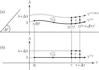
Figure 3: (a) The parameter manifold $M$ is symbolized by a horizontal plane while $\lambda$’s axis is seen in the vertical direction. The relevant paths $\gamma^{\scriptscriptstyle(\lambda)}$ are made at constant $\lambda$. It is shown in the text that the instantaneous pumped charge can be extracted from a loop $(\gamma^{\scriptscriptstyle(\lambda)}_{\tau,0})^{-1}\!\circ c\circ\gamma^{\scriptscriptstyle(\lambda)}_{\tau,0}$, where $c$ is a small rectangular loop oriented along the path and $\lambda$’s axis. (b) The effective space in variables $\tau$ and $\lambda$.

Let us first have a look at the charge pumped during an arbitrary small time interval $\Delta\tau$:

$$\Delta Q^{\scriptscriptstyle(r)}_{\rm g}(\tau)=i\,\mathfrak{F}^{\,r}_{\tau\lambda\;\,r}(\tau;\lambda)\,\Delta\tau+\Or\big{[}(\Delta\tau)^{2}\big{]}.$$

We may take advantage of formula (6) to compute the component $F_{\tau\lambda}(\tau;\lambda)$ in (11l). If we denote by $c$ the small rectangular loop pictured in figure 3, based at $(\tau;\lambda)$ with $\Delta\tau\sim\Delta\lambda\sim\Delta$, equality (11l) becomes:

$$\mathfrak{F}_{\tau\lambda}(\tau;\lambda) = W^{-1}\big{[}\gamma^{\scriptscriptstyle(\lambda)}_{\tau,0}\big{]}\frac{\leavevmode\hbox{\small 1\kern-3.8pt\normalsize 1}-W\big{[}c\big{]}}{\Delta\tau\Delta\lambda}\,W\big{[}\gamma^{\scriptscriptstyle(\lambda)}_{\tau,0}\big{]}+\Or\big{(}\Delta^{3}\big{)}$$

$$= \frac{1}{\Delta\tau\Delta\lambda}\Big{\{}\leavevmode\hbox{\small 1\kern-3.8pt\normalsize 1}\!-\!W\big{[}(\gamma^{\scriptscriptstyle(\lambda)}_{\tau,0})^{-1}\!\circ c\circ\gamma^{\scriptscriptstyle(\lambda)}_{\tau,0}\big{]}\Big{\}}\!+\!\Or\big{(}\Delta^{3}\big{)}.$$

Setting $\mathcal{C}$ the loop $(\gamma^{\scriptscriptstyle(\lambda)}_{\tau,0})^{-1}\!\circ c\circ\gamma^{\scriptscriptstyle(\lambda)}_{\tau,0}$ based at $(0;\lambda)$, one obtains an alternative formulation of the pumped charge:

$$\Delta Q^{\scriptscriptstyle(r)}_{\rm g}(\tau)=\frac{1}{\Delta\lambda}\,\Im\Big{\{}W^{\,r}_{\;\;r}\big{[}\mathcal{C}\big{]}\Big{\}}+\Or\big{(}\Delta^{2}\big{)}.$$ (11m)

Note that in the Abelian case $W\big{[}\mathcal{C}\big{]}$ is equal to $W\big{[}c\big{]}$ and the rectangle $c$ alone suffices for the computation. That represents geometrically the difference between the Abelian and non-Abelian pumpings, in terms of locality or non locality. Formula (11m), when combined with (8) and (9), is very useful for numerical purposes, as we will see later with an explicit example.

As a second step, we would like to derive a similar expression for finite $\Delta\tau$. To this end, we will consider the charge $Q_{\rm g}\big{[}\gamma^{\scriptscriptstyle(\lambda_{0})}_{\tau_{1},\tau_{0}}\big{]}$ pumped along $\gamma^{\scriptscriptstyle(\lambda_{0})}$ between any two times $\tau_{0}$ and $\tau_{1}$:

$$Q^{\scriptscriptstyle(r)}_{\rm g}\big{[}\gamma^{\scriptscriptstyle(\lambda_{0})}_{\tau_{1},\tau_{0}}\big{]}=i\int_{\tau_{0}}^{\tau_{1}}\mathfrak{F}^{\,r}_{\tau\lambda\;\,r}(\tau;\lambda_{0})\,{\rm d}\tau.$$ (11n)

Let $\{\zeta^{\scriptscriptstyle(\tau)}_{\lambda,\lambda_{0}}\,|\,(\tau,\lambda)\in[\tau_{0},\tau_{1}]\times I\}$ be the set of “vertical” segments oriented from $(\tau;\lambda_{0})$ to $(\tau;\lambda)$ in the effective space (see figure 4). Then, we define rectangular loops $c(\tau;\lambda)$ as follows:

$$c(\tau;\lambda):=(\zeta^{\scriptscriptstyle(\tau_{0})}_{\lambda,\lambda_{0}})^{-1}\circ(\gamma^{\scriptscriptstyle(\lambda)}_{\tau,\tau_{0}})^{-1}\circ\zeta^{\scriptscriptstyle(\tau)}_{\lambda,\lambda_{0}}\circ\gamma^{\scriptscriptstyle(\lambda_{0})}_{\tau,\tau_{0}}.$$

Setting $T(\tau;\lambda):=W\big{[}\gamma^{\scriptscriptstyle(\lambda)}_{\tau,\tau_{0}}\circ\zeta^{\scriptscriptstyle(\tau_{0})}_{\lambda,\lambda_{0}}\big{]}$, the Wilson loop $W\big{[}c(\tau;\lambda)\big{]}$ can be expressed as

$$W\big{[}c(\tau;\lambda)\big{]}=T^{-1}(\tau;\lambda)\,W\big{[}\zeta^{\scriptscriptstyle(\tau)}_{\lambda,\lambda_{0}}\big{]}\,T(\tau;\lambda_{0}),$$ (11o)

where we have noticed the property

$$T(\tau;\lambda_{0})=W\big{[}\gamma^{\scriptscriptstyle(\lambda_{0})}_{\tau,\tau_{0}}\big{]}.$$ (11p)

Thanks to the similarity rule (5), $W\big{[}c(\tau;\lambda)\big{]}$ in equation (11o) appears to be the image of $W\big{[}\zeta^{\scriptscriptstyle(\tau)}_{\lambda,\lambda_{0}}\big{]}$ under the gauge transformation generated by $T$ [47]. As for $A_{\lambda}$, it transforms according to the compatibility condition (4):

$$A_{\lambda}\mapsto\widetilde{A}_{\lambda}=T^{-1}A_{\lambda}\,T+T^{-1}\partial_{\lambda}T.$$

It is straightforward to verify that the partial derivative of $\widetilde{A}_{\lambda}$ with respect to $\tau$ is merely equal to $\widetilde{F}_{\tau\lambda}=T^{-1}F_{\tau\lambda}T$. Or, in the integral form:

$$\widetilde{A}_{\lambda}(\tau;\lambda)=\int_{\tau_{0}}^{\tau}T^{-1}(\tau^{\prime};\lambda)F_{\tau\lambda}(\tau^{\prime};\lambda)T(\tau^{\prime};\lambda)\,{\rm d}\tau^{\prime}.$$ (11q)

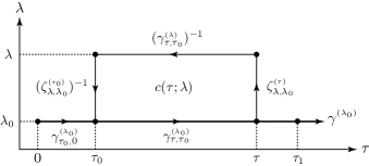
Figure 4: An illustration of the various oriented segments and loops defined in the text to compute the pumped charge between times $\tau_{0}$ and $\tau_{1}$.

The last result allows a curvature formulation of the Wilson loop $W\big{[}c(\tau;\lambda)\big{]}$, through a “$\lambda$-ordered” surface integral:

$$W\big{[}c(\tau;\lambda)\big{]} = \widetilde{W}\big{[}\zeta^{\scriptscriptstyle(\tau)}_{\lambda,\lambda_{0}}\big{]}=\mathcal{P}_{\lambda}\,e^{-\int_{\lambda_{0}}^{\lambda}\widetilde{A}_{\lambda}(\tau;\lambda^{\prime})\,{\rm d}\lambda^{\prime}}$$

$$= \mathcal{P}_{\lambda}\,\exp\Bigg{\{}\!\!-\frac{1}{2}\,\int_{\Sigma(\tau;\lambda)}\!\!\!\!\!T^{-1}F_{\tau\lambda}T\;{\rm d}\tau\wedge{\rm d}\lambda\Bigg{\}},$$

where $\Sigma(\tau;\lambda)$ is the well-oriented rectangular surface suspending the loop $c(\tau;\lambda)$ in the effective space. This is en passant an apparition of the so-called non-Abelian Stokes theorem [47, 46]. The connection between the pumped charge (11n) and our loops is established when taking $c(\tau_{1};\lambda)$ for a small difference $\Delta\lambda:=\lambda-\lambda_{0}$:

$$W\big{[}c(\tau_{1};\lambda)\big{]}=\mathcal{P}_{\lambda}\,e^{-\int_{\lambda_{0}}^{\lambda_{0}+\Delta\lambda}\widetilde{A}_{\lambda}(\tau_{1};\lambda^{\prime})\,{\rm d}\lambda^{\prime}}=\leavevmode\hbox{\small 1\kern-3.8pt\normalsize 1}-\widetilde{A}_{\lambda}(\tau_{1};\lambda_{0})\,\Delta\lambda+\Or\big{[}(\Delta\lambda)^{2}\big{]}.$$

Using equation (11q) and property (11p), one obtains

$$W\big{[}c(\tau_{1};\lambda)\big{]}=\leavevmode\hbox{\small 1\kern-3.8pt\normalsize 1}\!-\!\Delta\lambda\!\!\int_{\tau_{0}}^{\tau_{1}}\!\!\!W^{-1}\big{[}\gamma^{\scriptscriptstyle(\lambda_{0})}_{\tau,\tau_{0}}\big{]}F_{\tau\lambda}(\tau;\lambda_{0})W\big{[}\gamma^{\scriptscriptstyle(\lambda_{0})}_{\tau,\tau_{0}}\big{]}{\rm d}\tau+\Or\big{[}(\Delta\lambda)^{2}\big{]}.$$ (11r)

We set $\mathcal{C}=(\gamma^{\scriptscriptstyle(\lambda)}_{\tau_{0},0})^{-1}\circ c(\tau_{1};\lambda)\circ\gamma^{\scriptscriptstyle(\lambda)}_{\tau_{0},0}$, whose corresponding Wilson loop, deduced from (11r) and (11l), is

$$W\big{[}\mathcal{C}\big{]}=\leavevmode\hbox{\small 1\kern-3.8pt\normalsize 1}-\Delta\lambda\!\int_{\tau_{0}}^{\tau_{1}}\!\!\mathfrak{F}_{\tau\lambda}(\tau;\lambda_{0})\,{\rm d}\tau+\Or\big{[}(\Delta\lambda)^{2}\big{]}.$$ (11s)

After comparing (11s) with (11n) and using again anti-Hermiticity of $\mathfrak{F}_{\tau\lambda}$, one obtains the final expression:

$$Q^{\scriptscriptstyle(r)}_{\rm g}\big{[}\gamma_{\tau_{1},\tau_{0}}^{\scriptscriptstyle(\lambda_{0})}\big{]}=\frac{1}{\Delta\lambda}\,\Im\Big{\{}W^{\,r}_{\;\;r}\big{[}\mathcal{C}\big{]}\Big{\}}+\Or(\Delta\lambda).$$ (11t)

We achieved our purpose: computations of pumped charges need in any case a simple Wilson loop evaluation by way of relation (8). Let us conclude this section with a consideration on loops in parameter manifold: non-Abelian charge pumping will give rise to non-commuting loops in the sense that loops $\Gamma_{1}^{\scriptscriptstyle(\lambda)}$ and $\Gamma_{2}^{\scriptscriptstyle(\lambda)}$ based at the same point will generically be such that $Q^{\scriptscriptstyle(r)}_{\rm g}\big{[}\Gamma_{1}^{\scriptscriptstyle(\lambda)}\circ\Gamma_{2}^{\scriptscriptstyle(\lambda)}\big{]}\neq Q^{\scriptscriptstyle(r)}_{\rm g}\big{[}\Gamma_{2}^{\scriptscriptstyle(\lambda)}\circ\Gamma_{1}^{\scriptscriptstyle(\lambda)}\big{]}$. If $Q^{\scriptscriptstyle(r)}_{\rm g}\big{[}\Gamma_{1}^{\scriptscriptstyle(\lambda)}\big{]}$ and $Q^{\scriptscriptstyle(r)}_{\rm g}\big{[}\Gamma_{2}^{\scriptscriptstyle(\lambda)}\big{]}$ rely respectively on loops $\mathcal{C}_{1}$ and $\mathcal{C}_{2}$ in equation (11t), one can measure their “non-commutativity” through

$$Q^{\scriptscriptstyle(r)}_{\rm g}\big{[}\Gamma_{1}^{\scriptscriptstyle(\lambda)}\circ\Gamma_{2}^{\scriptscriptstyle(\lambda)}\big{]}-Q^{\scriptscriptstyle(r)}_{\rm g}\big{[}\Gamma_{2}^{\scriptscriptstyle(\lambda)}\circ\Gamma_{1}^{\scriptscriptstyle(\lambda)}\big{]}=\frac{1}{\Delta\lambda}\,\Im\Bigg{\{}\Big{[}W\big{[}\mathcal{C}_{1}\big{]},W\big{[}\mathcal{C}_{2}\big{]}\Big{]}^{r}_{\;\,r}\Bigg{\}}+\Or(\Delta\lambda).$$

Some experiments are already proposed to demonstrate the non-commutativity of pumping cycles [40, 34].

4 An illustrative example

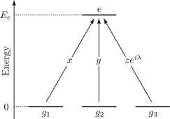
Figure 5: Relative couplings between the excited state $|e\rangle$ and the three ground states $|g_{1}\rangle$, $|g_{2}\rangle$ and $|g_{3}\rangle$, in the four-state model discussed in section 4.

We illustrate the results derived in the previous section with a well-known model appearing in atomic [9] and superconducting [34] systems. It consists of an excited state $|e\rangle$ parametrically coupled to three independent ground states $|g_{1}\rangle$, $|g_{2}\rangle$ and $|g_{3}\rangle$. In [34] the Hamiltonian reads

$$H(\bm{r};\lambda)=E_{e}|e\rangle\langle e|+x\,|e\rangle\langle g_{1}|+y\,|e\rangle\langle g_{2}|+z\,e^{i\lambda}\,|e\rangle\langle g_{3}|+{\rm h.c}.,$$

where $x$, $y$ and $z$ are three real parameters, $\bm{r}$ is the vector $(x,y,z)$ in the parameter space $\mathbb{R}^{3}$, and $E_{e}$ is the energy assigned to state $|e\rangle$ (eventually zero), while energies of the ground states are set to zero (see figure 5). In the context of [34], $H(\bm{r};\lambda)$ is a truncated Hamiltonian in the Coulomb blockade regime where $|e\rangle$, $|g_{1}\rangle$, $|g_{2}\rangle$ and $|g_{3}\rangle$ are the four relevant charge states (i.e. Cooper pairs in excess on different coupled islands). The parameters are then Josephson couplings between islands, the pumping parameter $\lambda$ is the phase bias between two superconducting leads and the current operator is the Cooper pair current from one lead to the other. Experimentally speaking, the parameters $x$, $y$ and $z$ live only in a restricted range of values. One may ask $\bm{r}$ to belong to a connected subset of $\mathbb{R}^{3}$ but this restriction is somewhat irrelevant. When $\bm{r}\neq\bm{0}$, the Hamiltonian has three distinct eigenvalues: $E_{-}$, $E_{0}\equiv 0$ and $E_{+}$, the second being doubly-degenerate over $\mathbb{R}^{3}\backslash\{\bm{0}\}$ while the non-degenerate eigenvalues $E_{\pm}$ depend only on $r:=\|\bm{r}\|=\sqrt{x^{2}+y^{2}+z^{2}}$:

$$E_{\pm}(r)=\frac{1}{2}\Big{(}E_{e}\pm\sqrt{E_{e}^{2}+4\,r^{2}}\Big{)}.$$

In the special case $\bm{r}=\bm{0}$, the level $E_{0}$ becomes at least three-fold degenerate: the origin is thus a defect for the ${\rm U}(2)$ gauge structure and we reduce the parameter space to $\mathbb{R}^{3}\backslash\{\bm{0}\}$. In order to perform non-Abelian pumping we focus on the eigenspaces associated with $E_{0}$. A smooth choice of orthonormal frame $\{|u_{1}\rangle,|u_{2}\rangle\}$ can be made over $\mathbb{R}^{3}\backslash(Oz)\times I$ as follows:

$$|u_{1}(\bm{r};\lambda)\rangle = \frac{y\,|g_{1}\rangle-x\,|g_{2}\rangle}{\sqrt{x^{2}+y^{2}}}$$ (11ua)

$$|u_{2}(\bm{r};\lambda)\rangle = \frac{-ze^{i\lambda}\big{(}x\,|g_{1}\rangle+y\,|g_{2}\rangle\big{)}+\big{(}x^{2}+y^{2}\big{)}|g_{3}\rangle}{\sqrt{(x^{2}+y^{2})(x^{2}+y^{2}+z^{2})}}\,.$$ (11ub)

A similar and compatible choice can also be found over e.g. $\mathbb{R}^{3}\backslash(Oy)\times I$ to cover entirely the parameter space:

$$|\tilde{u}_{1}(\bm{r};\lambda)\rangle = \frac{ze^{i\lambda}|g_{1}\rangle-x\,|g_{3}\rangle}{\sqrt{x^{2}+z^{2}}}$$

$$|\tilde{u}_{2}(\bm{r};\lambda)\rangle = \frac{-y\big{(}x\,|g_{1}\rangle+ze^{-i\lambda}|g_{3}\rangle\big{)}+\big{(}x^{2}+z^{2}\big{)}|g_{2}\rangle}{\sqrt{(x^{2}+z^{2})(x^{2}+y^{2}+z^{2})}}\,.$$

We note that all these states are invariant under a rescaling $\bm{r}\mapsto k\,\bm{r}$, $k>0$.

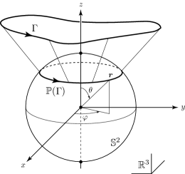
Figure 6: The charge pumped along a path $\Gamma$ in $\mathbb{R}^{3}$ is equal to the one pumped along $\Gamma$’s radial projection onto the unit sphere $\mathbb{S}^{2}$. Here, $\Gamma$ is a loop and its projection $\mathbb{P}(\Gamma)$ a circle.

Therefore, it is sufficient to retract $\mathbb{R}^{3}\backslash\{\bm{0}\}$ onto its embedded unit sphere $\mathbb{S}^{2}$: the pumped charge along a path $\gamma$ in $\mathbb{R}^{3}$ will be equal to the pumped charge along its radial projection $\mathbb{P}(\gamma)$ onto $\mathbb{S}^{2}$ (see figure 6). Using local spherical coordinates on $\mathbb{S}^{2}$: $\bm{r}=(\sin\theta\cos\varphi,\sin\theta\sin\varphi,\cos\theta)$, the eigenstates (11ua) and (11ub) read:

$$|u_{1}(\bm{r};\lambda)\rangle = \sin\varphi\,|g_{1}\rangle-\cos\varphi\,|g_{2}\rangle$$

$$|u_{2}(\bm{r};\lambda)\rangle = -e^{i\lambda}\cos\theta\big{(}\cos\varphi\,|g_{1}\rangle+\sin\varphi\,|g_{2}\rangle\big{)}+\sin\theta\,|g_{3}\rangle.$$

Within this choice, the components of the effective gauge fields have simple expressions:

$$A_{\tau}(\tau;\lambda) = -\cos[\theta(\tau)]\,\dot{\varphi}(\tau)\left(\begin{array}[]{cc}0&-e^{i\lambda}\\ e^{-i\lambda}&0\end{array}\right),$$

$$A_{\lambda}(\tau;\lambda) = i\cos^{2}[\theta(\tau)]\left(\begin{array}[]{cc}0&0\\ 0&1\end{array}\right),$$

and:

$$F_{\tau\lambda}(\tau;\lambda)=\frac{\sin[2\theta(\tau)]}{2\,i}\!\left(\begin{array}[]{cc}0&\sin[\theta(\tau)]\dot{\varphi}(\tau)e^{i\lambda}\\ \sin[\theta(\tau)]\dot{\varphi}(\tau)e^{-i\lambda}&2\dot{\theta}(\tau)\end{array}\right).$$

The simplicity of the above relations allows an exact computation of the Wilson line involved by the path followed between times 0 and $\tau$:

$$W\big{[}\gamma^{\scriptscriptstyle(\lambda)}_{\tau,0}\big{]}=\mathcal{P}_{\tau}\exp\Bigg{\{}-\int_{0}^{\tau}\!\!A_{\tau}(\tau;\lambda)\,{\rm d}\tau\Bigg{\}}=\left(\begin{array}[]{cc}\cos(\alpha_{\tau,0})&-e^{i\lambda}\sin(\alpha_{\tau,0})\\ e^{-i\lambda}\sin(\alpha_{\tau,0})&\cos(\alpha_{\tau,0})\end{array}\right)$$

where we set:

$$\alpha_{\tau,0}=\int_{0}^{\tau}\cos[\theta(\tau^{\prime})]\,\dot{\varphi}(\tau^{\prime})\,{\rm d}\tau^{\prime}=\int_{\gamma_{\tau,0}}\!\!\cos\theta\,{\rm d}\varphi.$$

One has thereby the basic ingredients to calculate via equation (11b) the transferred charges $Q^{\scriptscriptstyle(1)}_{\rm g}$ and $Q^{\scriptscriptstyle(2)}_{\rm g}$ along $\gamma^{\scriptscriptstyle(\lambda)}$. Namely,

$$Q_{\rm g}^{\scriptscriptstyle(1)}\big{[}\gamma^{\scriptscriptstyle(\lambda)}_{\tau,0}\big{]} = \sin^{2}(\alpha_{\tau,0})\sin^{2}[\theta(\tau)],$$ (11uya)

$$Q_{\rm g}^{(2)}\big{[}\gamma^{\scriptscriptstyle(\lambda)}_{\tau,0}\big{]} = \cos^{2}(\alpha_{\tau,0})\sin^{2}[\theta(\tau)]-\sin^{2}[\theta(0)].$$ (11uyb)

Note that they do not depend on $\lambda$’s magnitude; here, $\lambda$ is a pure pumping parameter with no observable effects. It is straightforward to check that, once the vertical Wilson line

$$W(\zeta^{\scriptscriptstyle(\tau)}_{\lambda+\Delta\lambda,\lambda})=\mathcal{P}_{\lambda}\exp\Bigg{\{}-\int_{\lambda}^{\lambda+\Delta\lambda}\!\!A_{\tau}(\tau;\lambda^{\prime})\,{\rm d}\lambda^{\prime}\Bigg{\}}=\left(\begin{array}[]{cc}1&0\\ 0&e^{-i\cos^{2}[\theta(\tau)]\Delta\lambda}\end{array}\right)$$

is obtained, formula (11t) yields to the same results (11uya) and (11uyb). In particular, if at time $T$ one has $\bm{r}(T)=\bm{r}(0)$, the path $\gamma^{\scriptscriptstyle(\lambda)}_{T,0}$ is a loop $\Gamma$ and the two pumped charges above are opposite: $Q_{\rm g}^{\scriptscriptstyle(1)}\big{[}\Gamma\big{]}=\sin^{2}(\alpha_{T,0})\sin^{2}[\theta(0)]=-Q_{\rm g}^{\scriptscriptstyle(2)}\big{[}\Gamma\big{]}$.

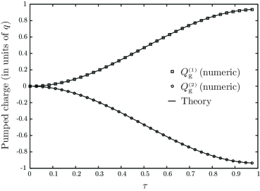
Figure 7: Analytical and numerical plots of the pumped charge in the circular example given in the text, for radius 1, $\cos\theta=1/4$ and $\lambda=0$. The algorithm is based on formulas (8) and (11m).

We conclude that section by a numerical test in the present non-Abelian example (for an Abelian case, see e.g. [23]). The algorithm is built on the discussion of subsection 2.2 applied to formula (11m). To check its validity, consider a mere situation: a circle whose axis is $(Oz)$ and such that $\cos\theta=1/4$. Whatever $\lambda$ be, if the circle is followed at constant velocity $\dot{\varphi}$ from $\tau=0$ to $\tau=1$, expressions (11uya) and (11uyb) become:

$$Q_{\rm g}^{\scriptscriptstyle(1)}\big{[}\gamma^{\scriptscriptstyle(\lambda)}_{\tau,0}\big{]}=\frac{15}{16}\,\sin^{2}\bigg{(}\frac{\pi}{2}\,\tau\bigg{)}=-Q_{\rm g}^{\scriptscriptstyle(2)}\big{[}\gamma^{\scriptscriptstyle(\lambda)}_{\tau,0}\big{]}.$$

In figure 7, the above expression together with the numerical result is plotted, and we find that they perfectly coincide.

5 Conclusion

We have shown the relevance of Wilson loops to describe adiabatic charge pumping, mainly for practical purposes. In that pure geometric approach, one may particularly take advantage of formulas (8) and (11m) to compute pumped charges in any problem. In the future, it should be interesting to investigate the geometry of this process in open systems, and to have a look at topological issues in the non-Abelian case.

Appendix. Curvature extraction from rectangles

In this appendix, we give a proof of formula (6). First of all, we denote by $x_{0}=x$, $x_{1}$, $x_{2}$ and $x_{3}$ the vertices of the oriented rectangle $c$, as depicted in figure 2, such that $x_{1}=x+\ell_{\mu}\,e_{\mu}$ and $x_{3}=x+\ell_{\nu}\,e_{\nu}$. Then, we decompose the loop into four oriented segments joining its vertices: $\ell_{10}$, $\ell_{21}$, $\ell_{32}$ and $\ell_{03}$, with $\ell_{kj}$ going from $x_{j}$ to $x_{k}$ (see figure 2). It suffices to treat $\ell_{10}$ and to apply the result to the others. This path can be parameterized as follows:

$$\ell_{10}:[0,1]\ni s\mapsto\ell_{10}(s)=x_{0}+s(x_{1}-x_{0})=x_{0}+s\,\ell_{\mu}\,e_{\mu}\in\mathbb{R}^{m}.$$

Within a gauge choice, its corresponding Wilson line reads:

$$W[\ell_{10}]=e^{-\int_{0}^{1}A_{\sigma}[\ell_{10}(s)]\frac{{\rm d}}{{\rm d}s}\big{[}\ell^{\sigma}_{10}(s)\big{]}{\rm d}s}=e^{-\ell_{\mu}\int_{0}^{1}A_{\mu}[\ell_{10}(s)]{\rm d}s}.$$

Expanding the path-ordered exponential as a usual Dyson series, one picks the expression of $W[\ell_{10}]$ up to the second order in $\ell_{\mu}$ (in a matrix norm sense):

$$W[\ell_{10}]=\leavevmode\hbox{\small 1\kern-3.8pt\normalsize 1}+\sum_{k=1}^{\infty}(-\ell_{\mu})^{k}\!\!\int_{0}^{1}\!\!{\rm d}s_{1}\!\int_{0}^{s_{1}}\!\!\!{\rm d}s_{2}\,\cdots\!\int_{0}^{s_{k-1}}\!\!\!\!{\rm d}s_{k}\Big{\{}A_{\mu}[\ell_{10}(s_{1})]A_{\mu}[\ell_{10}(s_{2})]\cdots A_{\mu}[\ell_{10}(s_{k})]\Big{\}}$$

$$\phantom{W[\ell_{10}]}=\leavevmode\hbox{\small 1\kern-3.8pt\normalsize 1}-\ell_{\mu}\int_{0}^{1}\!{\rm d}s\,A_{\mu}[\ell_{10}(s)]+\ell_{\mu}^{2}\int_{0}^{1}\!{\rm d}s\int_{0}^{s}\!{\rm d}s^{\prime}\,A_{\mu}[\ell_{10}(s)]A_{\mu}[\ell_{10}(s^{\prime})]+\Or\big{(}\ell_{\mu}^{3}\big{)}$$

$$\phantom{W[\ell_{10}]}=\leavevmode\hbox{\small 1\kern-3.8pt\normalsize 1}-A_{\mu}(x_{0})\,\ell_{\mu}+\frac{1}{2}\,\Big{\{}A^{2}_{\mu}(x_{0})-\partial_{\mu}A_{\mu}(x_{0})\Big{\}}\,\ell_{\mu}^{2}+\Or\big{(}\ell_{\mu}^{3}\big{)}\qquad{\rm or}$$

$$\phantom{W[\ell_{10}]}=\leavevmode\hbox{\small 1\kern-3.8pt\normalsize 1}-A_{\mu}(x_{1})\,\ell_{\mu}+\frac{1}{2}\,\Big{\{}A^{2}_{\mu}(x_{1})+\partial_{\mu}A_{\mu}(x_{1})\Big{\}}\,\ell_{\mu}^{2}+\Or\big{(}\ell_{\mu}^{3}\big{)}.$$

Therefore, the Wilson loop can be expressed as the product

$$W\big{[}c\big{]}=W\big{[}\ell_{03}\big{]}\cdot W\big{[}\ell_{32}\big{]}\cdot W\big{[}\ell_{21}\big{]}\cdot W\big{[}\ell_{10}\big{]}$$

$$\phantom{W\big{[}c\big{]}}=\phantom{\cdot}\,\bigg{(}\leavevmode\hbox{\small 1\kern-3.8pt\normalsize 1}+A_{\nu}(x_{0})\,\ell_{\nu}+\frac{1}{2}\,\Big{\{}A^{2}_{\nu}(x_{0})+\partial_{\nu}A_{\nu}(x_{0})\Big{\}}\,\ell_{\nu}^{2}\bigg{)}$$

$$\phantom{W\big{[}c\big{]}=}\cdot\bigg{(}\leavevmode\hbox{\small 1\kern-3.8pt\normalsize 1}+A_{\mu}(x_{3})\,\ell_{\mu}+\frac{1}{2}\,\Big{\{}A^{2}_{\mu}(x_{3})+\partial_{\mu}A_{\mu}(x_{3})\Big{\}}\,\ell_{\mu}^{2}\bigg{)}$$

$$\phantom{W\big{[}c\big{]}=}\cdot\bigg{(}\leavevmode\hbox{\small 1\kern-3.8pt\normalsize 1}-A_{\nu}(x_{1})\,\ell_{\nu}+\frac{1}{2}\,\Big{\{}A^{2}_{\nu}(x_{1})-\partial_{\nu}A_{\nu}(x_{1})\Big{\}}\,\ell_{\nu}^{2}\bigg{)}$$

$$\phantom{W\big{[}c\big{]}=}\cdot\bigg{(}\leavevmode\hbox{\small 1\kern-3.8pt\normalsize 1}-A_{\mu}(x_{0})\,\ell_{\mu}+\frac{1}{2}\,\Big{\{}A^{2}_{\mu}(x_{0})-\partial_{\mu}A_{\mu}(x_{0})\Big{\}}\,\ell_{\mu}^{2}\bigg{)}+\Or\big{(}\ell^{3}\big{)},$$

where $\ell$ stands for the order of the rectangle size: $\ell\sim\ell_{\mu},\ell_{\nu}$. Finally, using $A_{\nu}(x_{1})=A_{\nu}(x_{0})+\ell_{\nu}\partial_{\nu}A_{\nu}(x_{0})+\Or\big{(}\ell^{2}\big{)}$ and $A_{\mu}(x_{3})=A_{\mu}(x_{0})+\ell_{\mu}\partial_{\mu}A_{\mu}(x_{0})+\Or\big{(}\ell^{2}\big{)}$, one obtains

$$W\big{[}c\big{]} = \leavevmode\hbox{\small 1\kern-3.8pt\normalsize 1}-\Big{\{}\partial_{\mu}A_{\nu}(x_{0})-\partial_{\nu}A_{\mu}(x_{0})+\big{[}A_{\mu}(x_{0}),A_{\nu}(x_{0})\big{]}\Big{\}}\,\ell_{\mu}\ell_{\nu}+\Or\big{(}\ell^{3}\big{)}$$

$$= \leavevmode\hbox{\small 1\kern-3.8pt\normalsize 1}-F_{\mu\nu}(x)\,\ell_{\mu}\ell_{\nu}+\Or\big{(}\ell^{3}\big{)}.$$

References

References

- [1] Nakahara M 2003 Geometry, Topology and Physics (London: Taylor and Francis)
- [2] Berry M V 1984 Proc. R. Soc. A 392 45
- [3] Bleecker D 1981 Gauge Theory and Variational Principle (Reading, MA: Addison-Wesley)
- [4] Svetlichny G 1999 (Preprint math-ph/9902027)
- [5] Aharonov Y and Anandan J 1987 Phys. Rev. Lett. 58 1593
- [6] Simon B 1983 Phys. Rev. Lett. 51 2167
- [7] Wilczek F and Zee A 1984 Phys. Rev. Lett. 52 2111
- [8] Ekert A, Ericsson M, Hayden M, Inamori H, Jones H A, Oi D K L and Vedral V 2000 J. Mod. Opt. 47 2501 (Preprint quant-ph/0004015)
- [9] Recati A, Calarco T, Zanardi P, Cirac J I and Zoller P 2002 Phys. Rev. A 66 032309 (Preprint quant-ph/0204030)
- [10] Tomita A and Chiao R Y 1986 Phys. Rev. Lett. 57 937
- [11] Suter D, Chingas G C, Harris R A and Pines A 1987 Mol. Phys. 61 1327
- [12] Tycko R 1987 Phys. Rev. Lett. 58 2281–2284
- [13] Wernsdorfer W and Sessoli R 1999 Science 284 133
- [14] Leek P J, Fink J M, Blais A, Bianchetti R, Göppl M, Gambetta J M, Schuster D I, Frunzio L, Schoelkopf R J and Wallraff A 2007 Science 318 1889 (Preprint cond-mat/0711.0218)
- [15] Wilczek F and Shapere A 1989 Geometric Phases in Physics (Singapore: World Scientific)
- [16] Aharonov Y and Bohm D 1959 Phys. Rev. 115 485
- [17] King-Smith R D and Vanderbilt D 1993 Phys. Rev. B 47 1651
- [18] Resta R 1994 Rev. Mod. Phys. 66 899
- [19] Goryo J and Kohmoto M 2002 Phys. Rev. B 66 085118
- [20] Zak J 1989 Phys. Rev. Lett. 62 2747
- [21] Aunola M and Toppari J J 2003 Phys. Rev. B 68 020502 (Preprint cond-mat/0303176)
- [22] Möttönen M, Vartiainen J J and Pekola J P 2008 Phys. Rev. Lett. 100 177201 (Preprint cond-mat/0710.5623)
- [23] Leone R and Lévy L 2008 Phys. Rev. B 77 064524 (Preprint cond-mat/0711.0586)
- [24] Chang M C and Niu Q 1995 Phys. Rev. Lett. 75 1348 (Preprint cond-mat/9505021)
- [25] Chang M C and Niu Q 1996 Phys. Rev. B 53 7010 (Preprint cond-mat/9511014)
- [26] Sundaram G and Niu Q 1999 Phys. Rev. B 59 14915 (Preprint cond-mat/9908003)
- [27] Xiao D, Chang M C and Niu Q 2010 Rev. Mod. Phys. 82 1959 (Preprint cond-mat/0907.2021)
- [28] Goryo J and Kohmoto M 2008 Mod. Phys. Lett. B 22 303 (Preprint cond-mat/0606758)
- [29] Thouless D J 1983 Phys. Rev. B 27 6083
- [30] Thouless D J, Kohmoto M, Nightingale M P and den Nijs M 1982 Phys. Rev. Lett. 49 405
- [31] Kohmoto M 1985 Ann. Phys. 160 343
- [32] Keller M W 2008 Metrologia 102
- [33] Joye A, Brosco V and Hekking F 2010 (Preprint math-ph/1002.1223)
- [34] Brosco V, Fazio R, Hekking F W J and Joye A 2008 Phys. Rev. Lett. 100 027002 (Preprint cond-mat/0702333)
- [35] Pirkkalainen J M, Solinas P, Pekola J P and Möttönen M 2010 Phys. Rev. B 81 174506 (Preprint cond-mat/1002.0957)
- [36] Wendin G and Schumeiko V S 2005 (Preprint cond-mat/0508729)
- [37] Kato T 1950 J. Phys. Soc. Japan 5 435
- [38] Messiah A 1962 Quantum Mechanics vol 2 (Amsterdam: North-Holland)
- [39] Wilson K G 1974 Phys. Rev. D 10 2445
- [40] Zhou H Q, Cho S Y and McKenzie R H 2003 Phys. Rev. Lett. 91 186803
- [41] Pancharatnam S 1956 Proc. Ind. Acad. Sci. A 44 247–262
- [42] Bargmann V 1964 J. Math. Phys. 5 862
- [43] Press W, Flannery B, Teukolsky S and Vetterling W 1993 Numerical Recipes in Fortran 77: The Art of Scientific Computing vol 1 (Cambridge: Cambridge University Press)
- [44] Simon R and Mukunda N 1993 Phys. Rev. Lett. 70 880
- [45] Wang X, Vanderbilt D, Yates J R and Souza I 2007 Phys. Rev. B 76 195109 (Preprint cond-mat/0708.0858)
- [46] Broda B 2002 (Preprint math-ph/0012035)
- [47] Karp R L, Mansouri F and Rno J S 2000 Turk. Jour. Phys. 24 365 (Preprint hep-th/9903221)