Connecting Berry’s phase and the pumped charge in a Cooper pair pump

Abstract

The properties of the tunnelling-charging Hamiltonian of a Cooper pair pump are well understood in the regime of weak and intermediate Josephson coupling, i.e. when $E_{\mathrm{J}}\lesssim E_{\mathrm{C}}$. It is also known that Berry’s phase is related to the pumped charge induced by the adiabatical variation of the eigenstates. We show explicitly that pumped charge in Cooper pair pump can be understood as a partial derivative of Berry’s phase with respect to the phase difference $\phi$ across the array. The phase fluctuations always present in real experiments can also be taken into account, although only approximately. Thus the measurement of the pumped current gives reliable, yet indirect, information on Berry’s phase. As closing remarks, we give the differential relation between Berry’s phase and the pumped charge, and state that the mathematical results are valid for any observable expressible as a partial derivative of the Hamiltonian.

Josephson junction devices, e.g. Cooper pair box, superconducting single electron transistor (SSET) and Cooper pair pump (CPP), have been extensively studied both theoreticallyAverin (1998); Pekola et al. (1999); Makhlin et al. (1999); Averin (2000); Falci et al. (2000); Pekola and Toppari (2001) and experimentally.Eiles and Martinis (1994); Mooij et al. (1999); Nakamura et al. (1999); Orlando et al. (1999); Choi et al. (2001); Bibow et al. (2002) (For a recent review, see Ref. Makhlin et al., 2001.) Possible applications include coherent Cooper pair pumpingPekola et al. (1999) with related decoherence studiesNakamura et al. (1999); Pekola and Toppari (2001) or metrological applications,Hassel and Sepp$\ddot{\mathrm{a}}$ (1999) and the use of these devices as superconducting quantum bits (squbits) in quantum computation.Averin (1998); Mooij et al. (1999); Zhu and Wang (2002) In this paper we focus on CPP whose idealised tunnelling-charging Hamiltonian has been studied in detail in Refs. Pekola et al., 1999; Aunola et al., 2000; Aunola, 2001. For closed loops in the parameter space, we relate the pumped charge to Berry’s phase, a well-known geometrical phase attained by an adiabatically evolving eigenstate of a time-dependent Hamiltonian.Berry (1984); Simon (1983); Nakahara (1990) Some applications of geometrical phases in mesoscopic systems, are discussed in Refs. Falci et al., 2000; Chang and Simon, 1995 and the references therein. We illustrate the results both for the SSET and a CPP, and consider the effects due to phase fluctuations, present when experimentally measuring the pumped current.

In a CPP the pumping of Cooper pairs is induced by cyclic variation of the gate voltages while the evolution of the total phase difference across the array, $\phi$, is either fixed by ideal biasingPekola et al. (1999) or stochastically decoherent. Theoretical predictions are based on the adiabatic evolution of the eigenstates which splits the induced current into two parts: Pekola et al. (1999); Aunola et al. (2000) The direct supercurrent, which flows constantly and is proportional to the $\phi$-derivative of the dynamical phase of the eigenstate. The other part, the pumped charge, is explicitly induced by the action of pumping and proportional to the $\phi$-derivative of Berry’s phase for closed loops. Existence of such a relation was already implicitly stated in Ref. Pekola et al., 1999. The underlying reason for these connections is that the supercurrent operator $I_{\mathrm{S}}$ is an operator derivativeRudin (1973) of the full Hamiltonian with respect to $\phi$. This also implies that all of the results obtained in this paper are valid for any observable expressible as a partial derivative of the corresponding Hamiltonian. However, in real applications it might be reasonable to use the nonadiabatically attained geometrical phase instead of Berry’s phase.Zhu and Wang (2002)

A schematic view of a CPP is shown in Fig. 1. We assume that the gate voltages $V_{\mathrm{g},j}$ are independent and externally operated. The ideally operated bias voltage across the array, $V$, controls the total phase difference, $\phi$, according to $d\phi/dt=-2eV/\hbar$. In the absence of bias voltage, $\phi$ remains fixed and becomes a good quantum number.Ingold and Nazarov (1992); Pekola et al. (1999) Conversely, the conjugate variable $\hat{M}$, the average number of tunnelled Cooper pairs, becomes completely undetermined.

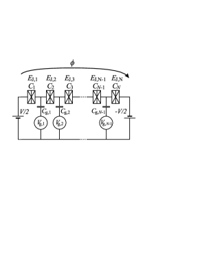
Figure 1: An ideal superconducting array of Josephson junctions (CPP). Here $C_{k}$ and $E_{\mathrm{J},k}$ are the capacitance and the Josephson energy of the $k^{\mathrm{th}}$ junction, respectively. The total phase difference across the array, $\phi$, is a constant of motion in the absence of the external bias voltage $V$.

The tunnelling-charging Hamiltonian

$$H=H_{\mathrm{C}}(\vec{q}\,)+H_{\mathrm{J}},$$ (1)

is assumed to be the correct description of the microscopic system, neglecting quasiparticle tunnelling as well as other degrees of freedom. The charging Hamiltonian $H_{\mathrm{C}}(\vec{q}\,)$ depends on the normalised gate charges, $\vec{q}:=(q_{1},\ldots,q_{N-1})$, and the number of Cooper pairs on each island, $\vec{n}=(n_{1},\ldots,n_{N-1})$, according to $\langle\vec{n}|H_{\rm C}(\vec{q}\,)|\vec{n}^{\prime}\rangle_{\phi}=E_{\rm C}(\vec{n}-\vec{q}\,)\delta_{\vec{n},\vec{n}^{\prime}}$. The function $E_{\rm C}(\vec{x})$ gives the details of the charging energy, see e.g. Ref. Aunola et al., 2000. The Josephson (tunnelling) Hamiltonian is given by

$$H_{\mathrm{J}}=-\sum_{k=1}^{N}E_{\mathrm{J},k}\cos(\phi_{k}),$$ (2)

where $E_{\mathrm{J},k}$ is the Josephson coupling energy of the $k^{\mathrm{th}}$ junction. The average supercurrent operator can be written in the form

$$I_{\mathrm{S}}=\frac{-2e}{N\hbar}\sum_{k=1}^{N}E_{\mathrm{J},k}\sin(\phi_{k})=\frac{-2e}{\hbar}\frac{\partial H}{\partial\phi},$$ (3)

where the operator derivativeRudin (1973) is defined as

$$\frac{\partial H}{\partial\phi}:=\lim_{\phi^{\prime}\rightarrow\phi}\frac{H(\phi^{\prime})-H(\phi)}{\phi^{\prime}-\phi}.$$ (4)

In the preferred representation, the parameter space is an $N$-dimensional manifold $\mathbb{R}^{N-1}\times S^{1}$, where the elements are of the form $\vec{p}=(\vec{q},\phi)$ with $\phi\in[0,2N\pi)$. For $N=2$, the system reduces to a SSET whose Hamiltonian is discussed in Ref. Tinkham, 1996. Asymptotically exact eigenvectors for strong Josephson coupling are given in Ref. Aunola, 2003.

We will study the adiabatic evolution of instantaneous energy eigenstates $|m\rangle$, while changing the gate voltages along a closed path $\Gamma:t\mapsto\vec{p}^{\,}(t)=(\vec{q}^{\,}(t),\phi(t))$ with $t\in[0,\tau]$. This induces a charge transfer $Q_{\mathrm{tot}}:=Q_{\mathrm{s}}+Q_{\mathrm{p}}$, where the pumped charge, $Q_{\mathrm{p}}$, depends only on the chosen path, $\Gamma$, determined by the gating sequence, while the charge transferred by the direct supercurrent, $Q_{\mathrm{s}}$, also depends on the rate of operation of the gate voltages, i.e., the value of $\tau$. The total transferred charge, in units of $-2e$, for state $|m\rangle$ becomesPekola et al. (1999); Aunola (2001)

$$Q_{\mathrm{tot}}=-\frac{\partial\eta_{m}}{\partial\phi}+2\oint_{\Gamma}{\rm Re}\left[\langle m|\hat{M}|dm\rangle\right].$$ (5)

Here $\hat{M}=-i\partial/\partial\phi$ is the operator for average number of tunnelled Cooper pairs, $\eta_{m}=-\int_{0}^{\tau}(E_{m}(t)/\hbar)dt$ is the dynamical phase and $|dm\rangle$ is the change in the eigenstate $|m\rangle$ due to a differential change $d\vec{p}=(d\vec{q},d\phi)$. A change $d\phi$ in the phase difference at $\vec{p}$ induces no pumped charge as we find $dQ_{p}=2{\rm Im}[\langle\hat{M}m|\hat{M}m\rangle]d\phi=0$. In other words, the bias voltage $V$ induces no pumped charge for fixed gate voltages.

The expression for $Q_{\mathrm{p}}$ is rather similar to the corresponding Berry’s phaseBerry (1984); Simon (1983)

$$\gamma_{m}(\Gamma)=i\oint_{\Gamma}\langle m|dm\rangle.$$ (6)

It should be stressed that Eqs. (5) and (6) are well defined also for open paths. The derivative $d$ in Eq. (6) is an exterior derivative so, for a closed path $\Gamma$, we may integrate Berry’s curvature over a two-surfaceNakahara (1990)

$$\gamma_{m}(\Gamma)=i\sum_{k=1}^{N}\sum_{l=1}^{N}\iint_{S_{\Gamma}}\frac{\partial\langle m|}{\partial q_{k}}\frac{\partial|m\rangle}{\partial q_{l}}dq_{k}\wedge dq_{l},$$ (7)

where the boundary of $S_{\Gamma}$ is the path $\Gamma$.int

We now construct an extended path for which Berry’s phase is proportional to the charge pumped along the path $\Gamma$. Let us define a class of closed paths $\{\Gamma_{\varphi}\}$ by $\Gamma_{\varphi}:t\mapsto\vec{p}^{\,}(t)=(\vec{q}^{\,}(t),\phi(t)+\varphi)$, where $t\in[0,\tau]$, so that $\Gamma_{0}=\Gamma$. The inverse of a path is the same path traversed in the opposite direction, which also holds for paths with distinct end points. We define an additional class of paths $\{\varphi_{\vec{p}}\}$ according to $\varphi_{\vec{p}}:t\mapsto(\vec{q},\phi+t\varphi)$, where $t\in[0,1]$. The extended path

$$\Gamma_{\mathrm{ext}}^{\varphi}:=\Gamma_{0}\circ\varphi_{\vec{p}\,(0)}\circ\Gamma_{\varphi}^{-1}\circ\varphi_{\vec{p}\,(0)}^{-1}$$ (8)

is also closed and spans a two-dimensional integration surface whose width in $\phi$-direction is $\varphi$. By traversing the boundary the contributions from $\varphi_{\vec{p}\,(0)}$ and $\varphi_{\vec{p}\,(0)}^{-1}$ naturally cancel, and we find

$$\gamma(\Gamma_{\mathrm{ext}}^{\varphi})=\gamma(\Gamma)-\gamma(\Gamma_{\varphi}).$$ (9)

Next we take the limit $\varphi\rightarrow 0$ and consider a strip of infinitesimal width $d\phi$ between $\Gamma_{d\phi}$ and $\Gamma_{0}$ as illustrated in Fig. 2.

Figure 2: A closed path $\Gamma$ has been flattened, i.e. the ends of $\Gamma$ meet. The infinitesimal pieces of length $d\phi$ are identical, but traversed in opposite directions. The two-dimensional integration surface $S_{\Gamma,d\phi}$ is spanned between orbits $\Gamma$ and $\Gamma_{d\phi}$. Berry’s phase corresponding to the boundary of $S_{\Gamma,d\phi}$ is identical to $-Q_{\mathrm{p}}(\Gamma)d\phi$, with $Q_{\mathrm{p}}(\Gamma)$ defined in Eq. (10).

This means that in Eq. (7) we have either $dq_{k}=d\phi$ or $dq_{l}=d\phi$ as the full length of integration and we can factor $d\phi$ from the expression for Berry’s phase. By rephrasing $Q_{\mathrm{p}}$ in Eq. (5) as

$$Q_{\mathrm{p}}(\Gamma)=i\sum_{k=1}^{N}\oint_{\Gamma}\left[\frac{\partial\langle m|}{\partial\phi}\frac{\partial|m\rangle}{\partial q_{k}}-\frac{\partial\langle m|}{\partial q_{k}}\frac{\partial|m\rangle}{\partial\phi}\right]dq_{k},$$ (10)

we see that it is identical to Berry’s phase in Eq. (7) apart from the factor $-d\phi$. By taking the limit from the equivalent result $\lim_{\varphi\rightarrow 0}(\gamma(\Gamma)-\gamma(\Gamma_{\varphi}))/\varphi$, we obtain the first main result

$$Q_{\mathrm{s}}+Q_{\mathrm{p}}=-\partial\eta_{m}/\partial\phi-\partial\gamma_{m}/\partial\phi.$$ (11)

This clearly shows the connection between Berry’s phase and the pumped charge, which is completely analogous with the connection between the dynamical phase and the accumulated charge due to direct supercurrent.

We now proceed in the opposite direction and consider strips of finite width instead of infinitesimal ones. By integrating the pumped charge with respect to $\phi$ over the set $\{\Gamma_{\varphi}\}$, we obtain the average pumped charge per cycle, $Q_{p,\mathrm{ave}}$, as

$$Q_{p,\mathrm{ave}}=\frac{1}{\varphi}\int_{0}^{\varphi}Q_{p}(\Gamma_{\phi})d\phi=\frac{\gamma(\Gamma_{0})-\gamma(\Gamma_{\varphi})}{\varphi}.$$ (12)

The graphical representation of this situation in a three-junction CPP and a SSET, are shown in Fig. 3 (I,II) and in Fig. 4, respectively. The cases are qualitatively different, because there is only one $q$-coordinate in a SSET.

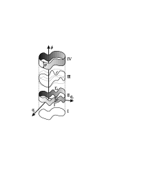
Figure 3: I) A projection of path $\Gamma$ in the $(q_{1},q_{2})$-plane. II) A strip of finite width $\varphi$ based on the path $\Gamma$. III) The fluctuations of $\phi$ on a single pumping cycle, $\ell$. IV) Ideal operation of gate voltages produces a strip bounded by the planes $\phi=\phi_{0}$ and $\phi=\phi_{0}+\varphi$. The same result is obtained approximately after many cycles with restricted, stochastic fluctuations of $\phi$.

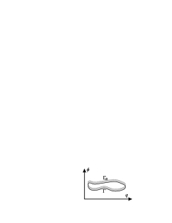
Figure 4: Pumping of Cooper pairs in SSET recuires also an ideal control of $\phi$. The projection of the path $\Gamma$ onto $q$-space is a line traversed back and forth.

We now wish to relate the above results to actual measurements of Cooper pair pumping. First, consider a closed path $\Gamma$ corresponding to a fixed value of $\phi_{0}$ as in Ref. Pekola et al., 1999. Under ideal operation of gate and bias voltages we can change $\phi$ slightly between each cycle and obtain a clean strip bounded by the planes $\phi=\phi_{0}$ and $\phi=\phi_{0}+\varphi$ as shown in Fig. 3 (IV). Combined with Eq. (12) this amounts to an important result for an ideal CPP: The measured pumped charge per cycle (i.e.  $Q_{p,\mathrm{ave}}$) yields direct information about differences of Berry’s phases.

Obtaining the same information in a real experiment is not so straightforward. Neither the phase difference, $\phi$, nor the gate voltages are ideally controlled. Nevertheless, we try to partially circumvent these problems using reasonable approximations. First, we assume that the gate voltages are operated accurately enough, so that the projections onto $q$-space nearly coincide. Additionally, $\phi$ fluctuates stochastically, but these fluctuations are restricted during time intervals shorter than the decoherence time, $\tau_{\phi}$.Pekola and Toppari (2001) For times larger than $\tau_{\phi}$ the fluctuations mount up too large and the phase coherence of the system is lost.

The decoherence is induced by any interaction between the quantum mechanical system and the environment. In a well prepared experiment, e.g. a CPP can be isolated from its surroundings so that the main contribution to $\tau_{\phi}$ is given by the electromagnetic environment in the vicinity of the sample and the effects due to finite temperature, restricting the measurements to subkelvin regime.

The decoherence time can be calculated theoretically from the fluctuation-dissipation –theorem as in Ref. Pekola and Toppari, 2001 or by looking at coherences, i.e., off-diagonal elements of the density matrix. The Hamiltonian in the presence of the electromagnetic environment reads

$$H=H_{\mathrm{C}}(q)+H_{\mathrm{J}}+H_{\mathrm{env}}+H_{\mathrm{int}},$$ (13)

where $H_{\mathrm{env}}=\sum_{j}(b_{j}^{\dagger}b_{j}+1/2)\hbar\omega_{j}$ and $b_{j}^{\dagger}$ and $b_{j}$ are the creation and annihilation operators of the bosonic environmental mode $j$ with energy $\hbar\omega_{j}$, respectively.Caldeira and Leggett (1983) As an example, we consider a SSET but it should be stressed that the result generalises for any number of junctions. We write the density matrix $\rho^{\vec{k}}=\Psi^{\vec{k}}\Psi^{\vec{k}{\dagger}}$ in the basis consisting of two SSET charge states, $\{|m\rangle\}_{m=0}^{1}$ and environmental modes $\{|\vec{k}=(k_{1},k_{2},\ldots)\rangle\}$. Then the Hamiltonian describing the interaction between SSET and the environment becomes Caldeira and Leggett (1983); Cottet et al. (2001)

$$H_{\mathrm{int}}=-i\sqrt{\pi}\sum\limits_{j}\hbar\omega_{j}\sqrt{\frac{Z_{j}}{R_{\mathrm{K}}}}\left(b_{j}-b_{j}^{\dagger}\right)\left(\begin{array}[]{cc}1&0\\ 0&-1\end{array}\right),$$ (14)

where $Z_{j}$ is the impedance of the mode $j$ and $R_{\mathrm{K}}=h/e^{2}\simeq 25.8$ k$\Omega$ is the resistance quantum.

The equation of motion for $\rho^{\vec{k}}_{\rm I}$ in the interaction picture is given by the Liouville equation, $i\hbar(d\rho^{\vec{k}}_{\mathrm{I}}(t)/dt)=[H_{\mathrm{int,I}}\,,\rho^{\vec{k}}_{\mathrm{I}}(t)]$. By solving the differential equation for the coherence matrix elements and tracing out the environmental configurations $\vec{k}$ we obtain the final result

$$\rho_{\mathrm{I},12}(t)=\rho_{\mathrm{I},12}(0)\exp\left[-2{\rm Re}J(t)\right],$$ (15)

which corresponds to the same time scale as given by the fluctuation-dissipation -6-theorem. Pekola and Toppari (2001) Here $J(t)$ is the phase-phase correlation function $J(t)=\langle\left[\varphi(t)-\varphi(0)\right]\varphi(0)\rangle$ and $\rho_{\mathrm{I}}=\langle\rho_{\mathrm{I}}^{\vec{k}}\rangle_{\vec{k}}\,$.Ingold and Nazarov (1992) In case of purely resistive electromagnetic environment, $R_{\mathrm{e}}$, Eq. (15) yields Pekola and Toppari (2001) $\tau_{\phi}\simeq[\pi\hbar/(16k_{\mathrm{B}}T)]R_{\mathrm{K}}/R_{\mathrm{e}}$, where we have assumed nonzero temperature and $\pi k_{\mathrm{B}}Tt/\hbar\gg 1$. For realistic measurement parameters, e.g. $T=10$ mK and $R_{\mathrm{e}}=10$ $\Omega$, one obtains a rather long time $\tau_{\phi}\simeq 0.4$ $\mu$s.

Returning to Berry’s phase, we assume an initial value $\phi_{0}$ and consider time intervals shorter than $\tau_{\phi}$, effectively restricting $\phi$ to a finite range $[\phi_{1},\phi_{2}]\ni\phi_{0}$. If sufficiently many (identical) cycles of gate voltages are performed during this time, the fluctuations of $\phi$ yield a relatively thick mesh of trajectories within the strip. Although the ’weights’ for different values of $\phi$ are uneven, we approximate the mesh with a uniform distribution which is a subset of the range $[\phi_{1},\phi_{2}]$. This corresponds to a well-defined strip as in the ideal case of Eq. (12) and is presented in Fig. 3 (IV). A cycle, $\ell$, with exaggerated fluctuations in $\phi$, is shown in Fig. 3 (III). Due to the stochastic nature of the fluctuations, it is impossible to predict the correct range to be used. Nevertheless, for periods that are short enough, the correspondence between Berry’s phase and the measured pumped charge exists in the sense of Eq. (12). If the end points of the full pumping cycle are sufficiently close, Eq. (11) is valid, at least in the framework of the model.

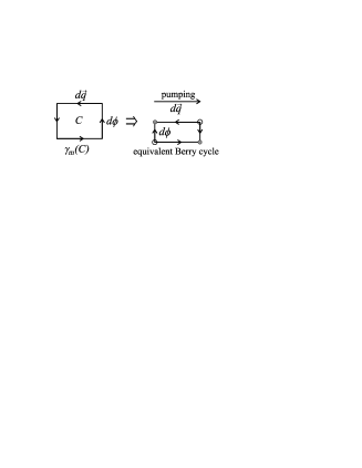
Figure 5: An infinitesimal cycle $C$ corresponding to Berry’s phase $\gamma_{m}(C)$ consists of four legs. The charge transfer $Q_{\rm p}$ for a fixed $\phi$ is identical to Berry’s phase induced by traversing the legs in the directions shown on the right-hand-side divided by $d\phi$. This path can not be continuously followed in the parameter space.

As a final note, we construct the differential relation between Berry’s phase and the pumped charge. Let us consider Berry’s phase $\gamma_{m}$ induced by an infinitesimal closed cycle $C$ at $(\vec{q},\phi)$ with sides $d\vec{q}$ and $d\phi$ as shown by the left-hand-side of Fig. 5. On the right-hand-side, the pumped charge due to $d\vec{q}$ multiplied by $d\phi$, is identical to Berry’s phase induced by the discontinuous path below it. By following any closed pumping path $\Gamma$ and integrating the pumped charge, we recover Eq. (11). If the path is not a closed one, a nontrivial integration with respect to $\phi$ remains, regardless of the width of the strip.

In conclusion, we have shown explicitly how the pumped charge in Cooper pair pump can be understood as a partial derivative of Berry’s phase with respect to the phase difference $\phi$ across the array. We have only used the fact that the supercurrent operator $I_{\mathrm{S}}$ is an operator derivative of the full Hamiltonian. Thus these results generalise for any observable with this property. We have also shown how one could obtain information about Berry’s phase by measuring the pumped current in a CPP.