On the type of the temperature phase transition in $\phi^{4}$ model

Abstract

The temperature induced phase transition is investigated in the one-component scalar field $\phi^{4}$ model on a lattice by using Monte Carlo simulations. Using the GPGPU technology a huge amount of data is collected that gives a possibility to determine the Linde-Weinberg low bound on the coupling constant $\lambda_{0}$ and investigate the type of the phase transition for a wide interval of coupling values. It is found that for the values of $\lambda$ close to this bound a weak-first-order phase transition happens. It converts into a second order phase transition with the increase of $\lambda$. A comparison with analytic calculations in continuum field theory and lattice simulations obtained by other authors is given.

Keywords: scalar model; phase transitions; GPU

1 Introduction

The temperature induced phase transition in the $O(N)$ scalar field model with a spontaneous symmetry breaking (SSB) has a long history of investigations. It was studied either by analytic methods of the quantum field theory or in lattice simulations (see Refs.[1, 2, 3] and references therein). It was recently observed by analytic calculations within the perturbation theory (PT) in the daisy, super daisy and some type beyond resummations [4] that a phase transition of the first order could occur in the $O(1)$-model. However, the lack of the expansion parameter happens near the phase transition temperature $T\sim T_{c}$ for various kind resummations. So, it is impossible to draw a reliable conclusion about the transition type even for small values of the coupling constant $\lambda$. In Ref.[5] some extended kind of resummations were used for the $O(N)$-model, and a phase transition of the second order was determined independently of the coupling value. Analogous results have been obtained in Monte Carlo (MC) simulations on a lattice. As a result, nowadays the general believe is that the phase transition is of the second order and the PT fails in this problem. However, in the $O(N)$-models, the results of PT calculations coincide with the lattice MC ones in the limit of $N\to\infty$, only [4, 6].

Recently, a new powerful computational platform – General Purpose computing on Graphics Processing Units (GPGPU) technology – has been put in force [9, 10] that gives a possibility to generate extremely large amount of MC data. Therefore the accuracy of calculations can be essentially increased and it becomes possible to shed light upon hidden peculiarities and details of different processes of interest studied by MC simulations. One of such unsolved problems is the kind of the temperature phase transition in the $O(1)$-model for small values of $\lambda$ and the reliability of the PT results. This is because there are no estimates what coupling values should be considered as small ones. As a rule, the small values are chosen to be of the order $\lambda\sim 0.1-0.01$. However, to make the correct choice some physical motivation is needed. One of possible reasons is the so-called Linde-Weinberg bound on the scalar field mass [7, 8]. Many years ago these authors observed that in models with the negative mass squared, $m^{2}\leq 0$, the SSB did not happen for the coupling values below some scale, $\lambda\leq\lambda_{0}$. The actual value $\lambda_{0}$ depends on the mass parameter entering the Lagrangian. So, it is natural to consider the values of the coupling $\lambda\sim\lambda_{0}$ as small ones. These values appear to be much smaller than the values mentioned above.

In the present paper we investigate the temperature induced phase transition in the $O(1)$-model in a wide interval of the coupling constant $\lambda$ using the GPGPU technology. We obtain the Linde-Weinberg bound $\lambda_{0}\sim 10^{-5}$. Then we compare the MC simulations with the hot and cold starts. In a narrow interval just above the Linde-Weinberg bound, $\lambda_{0}\leq\lambda~{}\leq\lambda_{1}\simeq 10^{-3}$, an order parameter shows a hysteresis behavior near the phase transition temperature. This behavior means a phase transition of the first order. With the further increasing of $\lambda$ the hysteresis behavior becomes less pronounced and disappears at all reflecting a phase transition of the second order.

The paper is organized as follows. In sect.2 we describe the model and its realization on a lattice. In sect.3 a necessary information on the MC simulations is given and the obtained results are adduced. Sect.4 summarizes the results.

2 The model

In order to construct a self-consistent lattice version of the $\phi^{4}$-model we start with quantum field theory in continuous space. The thermodynamical properties of the model are described by the generating functional

$$Z=\int D\varphi~{}e^{-S[\varphi]},$$ (1)

where $\varphi$ is a real scalar field, and the action is

$$S=\int dx\left(\frac{1}{2}\partial_{\mu}\varphi(x)\partial_{\mu}\varphi(x)-\frac{1}{2}m^{2}\varphi(x)^{2}+\frac{\lambda}{4}\varphi(x)^{4}\right).$$ (2)

The standard realization of generating functional in MC simulations on a lattice assumes a space-time discretization and the probing random values of fields in order to construct the Boltzmann ensemble of field configurations. Then any macroscopic observable can be measured by averaging the corresponding microscopic quantity over this ensemble. However, the direct lattice implementation of (1) encounters an evident problem: the field $\varphi$ is distributed uniformly in the infinite interval $(-\infty,\infty)$ and there is no random number generator to simulate it. Of course, one can try to cut the interval off, but such a procedure requires the knowledge of characteristic scales of the model in order to separate the unimportant tails from the interval of physically important values. Instead, we prefer to rewrite the initial $\phi^{4}$ model in continuum space-time in the form allowing a further self-consistent lattice realization.

First we introduce one-to-one transformation $\varphi(U)$ to a new field variable $U(x)$ defined in the finite interval $(0,1)$. Let $U=0.5$ corresponds to $\varphi=0$ and $\varphi(U)=-~{}\varphi(1-U)$. The generating functional in terms of $U$ reads

$$Z=\int DU\ \det\left(\frac{\partial\varphi}{\partial U}\right)~{}e^{-S[\varphi(U)]}.$$ (3)

The Jacobian can be included in the action as $\det A=\exp(\mathrm{Tr}\log A)$. Then the new field $U$ can be easily realized by a uniform random number generator.

The second step is the space-time discretization. For MC simulations we introduce a hypercubic lattice with hypertorous geometry. We use an anisotropic lattice with the spatial and temporal spacings $a_{s}$ and $a_{t}=a_{s}/\zeta$, $\zeta>1$. The scalar field is defined in the lattice sites. As a result, the generating functional becomes

$$Z=\int\prod_{x}dU(x)\exp{\left[-\left(S[\varphi(U(x))]-\sum_{x}\log\varphi^{\prime}[U(x)]\right)\right]},$$ (4)

where $\varphi^{\prime}(U)=d\varphi/dU$ and

$$S[\varphi(U(x))]=$$

$$\sum_{x}\frac{a_{s}^{4}}{\zeta} \left[\left(\varphi^{\prime}[U(x)]\right)^{2}\frac{\partial_{\mu}U(x)\partial_{\mu}U(x)}{2}-\frac{m^{2}}{2}\varphi^{2}[U(x)]+\frac{\lambda}{4}\varphi^{4}[U(x)]\right].$$ (5)

The lattice forward derivative is defined as usually by the finite difference operation

$$\partial_{\mu}U(x)\to\frac{U(x+a_{\mu}\hat{\mu})-U(x)}{a_{\mu}},$$ (6)

where $a_{\mu}$ is the lattice spacing in the $\mu$ direction, $\hat{\mu}$ is the unit vector in the direction indicated by $\mu$.

In the case of pure condensate field the action is determined by the potential

$$\tilde{V}[U]=\left[-\log\varphi^{\prime}[U]+\frac{a_{s}^{4}}{\zeta}\left(-\frac{1}{2}m^{2}\varphi^{2}[U]+\frac{\lambda}{4}\varphi^{4}[U]\right)\right].$$ (7)

This potential is topologically equivalent to the potential $V(\varphi)=-m^{2}\varphi^{2}/2$ $+\lambda\varphi^{4}/4$. It has one local maximum at $U=0.5$ and two symmetric global minima at $U_{0}$ and $1-U_{0}$. The spread between the values of the potential at the local maximum and the global minima is

$$\Delta_{V}=\log\frac{\varphi^{\prime}[U_{0}]}{\varphi^{\prime}[0.5]}-\frac{a_{s}^{4}}{\zeta}\left(-\frac{1}{2}m^{2}\varphi^{2}[U_{0}]+\frac{\lambda}{4}\varphi^{4}[U_{0}]\right).$$ (8)

The quantities $U_{0}$ and $\Delta_{V}$ play a crucial role in MC simulations. Being equivalent in theory, different choices of these parameters can produce drastically different results in actual simulations. The reason is the finite number of simulations in an actual computer experiment. If rare but physically important events could be missed, then the MC algorithm will not converge to the Boltzmann ensemble of configurations. In case of $\sim 10^{3}$ iterations all the important probabilities have to be greater than $10^{-3}$.

Considering the phase transition, one must guarantee that the MC algorithm meets the field values compatible with both the phases to choose. If $U_{0}\to 0.5$, then the broken phase can be missed since the corresponding field values are extremely rare events. On the other hand, in the limit $U_{0}\to 0$ (or $U_{0}\to 1$) the unbroken phase is washed out. It is also important to ensure a finite probability of the transition between those field values. The acceptance of non-zero condensate values of the field is ruled approximately by $\exp{(\Delta_{V})}$ at each lattice site. If $\Delta_{V}\gg 1$, then the unbroken phase never occurs in actual simulations. If $\Delta_{V}\to 0$, then there is no broken phase. To study the phase transition in the model, we choose the following conditions:

$$U_{0}=0.25,\qquad\Delta_{V}=1.$$ (9)

Thus, the half of generated field values will be between the global minima of the ‘effective’ potential, and no phase will be accidentally missed. The probability to prefer condensate or non-condensate values will be of order $\sim 0.5$ ensuring the fast convergence of MC algorithm. Of course, the choice (9) is not optimal for temperatures far away from the critical temperature.

To satisfy two conditions (9) we use a convenient two-parameter function,

$$\varphi[U] = m\xi\mathrm{arctanh}\left[\eta(2U-1)+(1-\eta)(2U-1)^{3}\right]$$ (10)

with $\xi>0$ and $\eta>0$. The values of $\xi$ and $\eta$ have to be found as the solution of equations $d\tilde{V}/dU|_{U=U_{0}}=0$ and (8). These equations can be written as

$$\frac{2{\cal F}[U_{0}]-{\cal G}[U_{0}]}{\left({\cal F}[U_{0}]-{\cal G}[U_{0}]\right)^{2}}=z=\frac{\lambda\zeta}{m^{4}a_{s}^{4}},$$ (11)

$$\frac{\lambda}{m^{2}z}\varphi^{2}[U_{0}]={\cal F}[U_{0}]-{\cal G}[U_{0}],$$ (12)

where $z$ is a dimensionless parameter of the model,

$${\cal K}[U] = \frac{1-\eta(2U-1)-(1-\eta)(2U-1)^{3}}{1+\eta(2U-1)+(1-\eta)(2U-1)^{3}},$$ (13)

$${\cal F}[U] = \left(\frac{{\cal K}^{\prime\prime}[U]{\cal K}[U]}{({\cal K}^{\prime}[U])^{2}}-1\right)\log{\cal K}[U],$$ (14)

$${\cal G}[U] = 4\left(\log\frac{-{\cal K}^{\prime}[U]}{4\eta{\cal K}[U]}-\Delta_{V}\right),$$ (15)

where the primes denote derivatives with respect to $U$. Eq. (11) gives $\eta(z)$, then $\xi$ can be found from (12). There is no physical solution for $z<z_{\mathrm{min}}$. This forbidden interval corresponds to low temperatures which cannot be reached within the chosen parametrization. Finally the lattice action is

$${S}[U(x)] = \sum_{x}\sum\limits_{\mu}\left[Y\sqrt{\frac{z}{\zeta\lambda}}\left(\frac{{\cal K}^{\prime}[U(x)]}{{\cal K}[U(x)]}\right)^{2}\left(\frac{U(x+a_{\mu}\hat{\mu})-U(x)}{a_{\mu}/a_{s}}\right)^{2}\right]$$

$$+ \sum_{x}\left[-\frac{1}{4}{\cal G}[U(x)]-Y\log^{2}{\cal K}[U(x)]+Y^{2}z\log^{4}{\cal K}[U(x)]+V_{0}\right],$$

$$Y = \frac{{\cal F}[U_{0}]-{\cal G}[U_{0}]}{2\log^{2}{\cal K}[U_{0}]},$$ (16)

$$V_{0} = -\Delta_{V}-\log(2m\xi\eta).$$ (17)

The constant part of the action $V_{0}$ is completely unimportant for calculations and can be omitted, since MC algorithm is based on the difference between the actions of modified and initial field configurations.

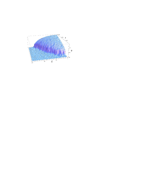
Figure 1: $|\bar{\varphi}|$ in the units of classical condensate $m/\sqrt{\lambda}$ for $\lambda=5\cdot 10^{-4}$ on lattice $16^{4}$

By varying $\zeta$ it is possible to change $a_{t}$, while keeping $a_{s}$ fixed. Consequently the temperature $T\sim\zeta$ can be changed continuously at the fixed $a_{s}$. At low temperatures the global discrete symmetry $\varphi\to-\varphi$ is expected to be broken due to a non-zero field condensate. The field condensate, $\bar{\varphi}$, can be measured directly as the average of $\varphi(x)$ over the lattice. As an example, in Fig.1 we plot $|\bar{\varphi}|$ in the units of the classical condensate $m/\sqrt{\lambda}$ for $\lambda=5\cdot 10^{-4}$ and $16^{4}$ lattice. The lower values of $\zeta$ and $z$ correspond to lower temperatures. One can see the evident phase transition with the field condensate growing with the temperature decreasing. Since the clear positive or negative values of $\bar{\varphi}$ appear in lattice configurations in the broken phase, we conclude about the absence of domains and will use $|\bar{\varphi}|$ in plots in what follows.

The field condensate is an obvious order parameter vanishing in the high-temperature phase. We can use it to determine the type of the phase transition. In case of the first-order transition the overheated and supercooled states are possible. So, the MC simulations with the hot and cold starts have to lead to different phases near the critical temperature. Combining the MC simulations for the hot and cold starts we will see a hysteresis plot. This exfoliation in the vicinity of the critical temperature has to be observed independently of the direction in the $(\zeta-z)$ plane.

We consider in details two slices of the two-dimensional function in Fig.1 at fixed $z=0.35$ and $z=0.5$. We compute the field condensate with the hot and cold starts for different $\zeta$. The hysteresis-type plots will mean a first order phase transition.

3 Monte Carlo simulation results

The exfoliation of the simulated data in the vicinity of the critical temperature is a tiny effect. A large amount of simulation data must be prepared to observe it. In this regard, achieving the highest performance of the computational hardware is a problem of great importance. To speed up essentially the simulation process we apply a GPU cluster of AMD/ATI Radeon GPUs: HD5870, HD5850, HD4870 and HD4850. The peak performance of the cluster is up to 8 Tflops. The low-level AMD Intermediate Language (AMD IL) is used in order to obtain the maximal performance of the hardware. Some technical details of MC simulations on the ATI GPUs and review of AMD Stream SDK are given in Ref. [9] and references therein.

The MC simulations are realized at hypercubic lattices up to $64^{4}$. Most of the obtained statistics come from the lattice $16^{4}$. We use the pseudo-random number generator RANLUX in the MC kernel, but all the key results are checked with RANMAR generator [10]. The lattice data are stored with the single precision. Updating the MC configurations are also performed with the single precision, whereas all the averaging measurements are carried out with the double precision to avoid the accumulation of errors.

It should be noted that for a rough estimate of the parameter space in the early stages of the work we used a pseudorandom number generator XOR128 to speed up the calculations. The condensate values obtained by this generator coincide with the correspondent points produced with the help of RANMAR and RANLUX generators. However, the generator XOR128 realized the two minima of the broken phase with an unequal frequency. Its unexpected behavior had been discovered in the first time, since good statistical properties of this generator were reported in the literature on real modeling before.

The system is thermalized by passing 5000 MC iterations for every run. For measuring we use 1024 MC configurations separated by 10 bulk updates.

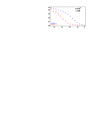
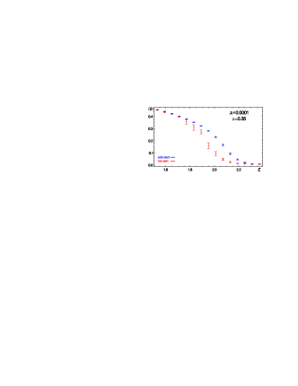
Figure 2: Temperature dependence of the absolute value of the averaged field $|\bar{\varphi}|$ for the lattice $16^{4}$ at $z=0.35$ and $z=0.5$ for $\zeta=[1.5;2.4]$.

As it was discussed in the previous section, we collect the data for the absolute value of the averaged field $|\bar{\varphi}|$ representing the field condensate. The temperature dependence of $|\bar{\varphi}|$ for the lattice $16^{4}$ at $z=0.35$ and $z=0.5$ for $\zeta=[1.5;2.5]$ is shown in Fig.2. The whole data set for every plot is divided into 15 bins. Different initial conditions are marked with different colors: the hot start is depicted in red (lower bins) and the cold start is represented in blue (upper bins). The mean values and the 95% confidence intervals are shown for each bin. Every bin contains 150 simulated points.

As it is seen from Fig.2, for $\lambda=0.01$ the temperature dependence of the field condensate is insensitive to the start configuration chosen. Both the cold and hot starts lead to the same behavior of the field condensate for various $\zeta$. This means the phase transition to be of the second order, and this result is in agreement with the common opinion on the type of the phase transition stated in Refs. [1, 2, 5]. However, therein this value of the coupling is considered as a small one.

Then, for smaller values of $\lambda$ the overheated configurations occur in the broken phase for the hot start, and the supercooled states can be found for the cold start. That is, the exfoliation of the simulated data in the vicinity of the critical temperature is observed for different start configurations. Such a hysteresis behavior corresponds to the phase transition of the first order.

With further decreasing of $\lambda$ to the values of order $\lambda_{0}\sim 10^{-5}$ the behavior of hot- and cold-started simulations becomes completely separated and independent of the temperature. This effect is plotted in Fig.3. Such type property means that the SSB does not happen even at zero temperature. The corresponding value $\lambda_{0}$ can be identified as the Linde-Weinberg low bound.

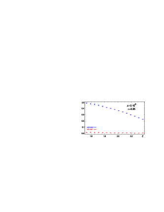
Figure 3: The Linde-Weinberg regime for the lattice $16^{4}$ at $\lambda=10^{-5},~{}5\cdot 10^{-6}$, $z=0.35$ and $\zeta=[1.5;2.4]$.

Comparing the plots for two different values of $z$ with the same set of other parameters in Fig.2, one can see that the hysteresis behavior for $z=0.5$ is similar to the case of $z=0.35$. This is the common feature for all the tested values of $\lambda$, but we adduce only one slide for brevity. The independence of $z$ is important. It means that the observed exfoliation of simulated points is stable within our parametrization of the action. Thus, the introduced approach is reliable at the transition temperature.

4 Conclusion

As it was discovered in MC simulations, the temperature phase transition in the $O(1)$ $\phi^{4}$ model is strongly dependent on a coupling value $\lambda$. There is the low bound $\lambda_{0}\sim 10^{-5}$ determining the range where the SSB is not realized. Close to this value in the interval $10^{-5}\leq\lambda\leq 10^{-3}$ the phase transition is of the first order. For larger values of $\lambda$ the second order phase transition happens. These observations, in particular, may serve as a criterium for applicability of different kind resummations in perturbation theory. In fact, we see that the daisy and super daisy resummations give qualitatively correct results for small values of $\lambda$. For larger values they become non-adequate to the second-order nature of the phase transition. In this case other more complicated resummation schemes should be used.

Acknowledgements. One of us (VD) was supported by DFG under Grant No BO1112/17-1. He also thanks Institute for Theoretical Physics of Leipzig University for kind hospitality.

References

- [1] Jean Zinn-Justin, Quantum field theory and critical phenomena, Clarendon Press, 1996.
- [2] J. Berges, N. Tetradis and C. Witterich, Phys.Rept.363, 223 (2002).
- [3] P. Cea, M. Comsoli and L. Cosmai, arXiv:hep-lat/0407024; arXiv:hep-ph/0311256; Nucl. Phys. Proc. Suppl. 106, 953 (2002) [arXiv:hep-lat/0110008].
- [4] M. Bordag and V. Skalozub, J. Phys. A 34, 461 (2001) [arXiv:hep-th/0006089]; Phys.Rev. D 65, 085025,2002, [arXiv:hep-th/0107027 v2].
- [5] J. Baacke and S. Michalski, Phys. Rev. D 67, 085006 (2003) [arXiv:hep-ph/0210060].
- [6] N. Petropoulos arXiv:hep-ph/0402136.
- [7] A. D. Linde, JETP Lett. 23, 64 (1976) [Pisma Zh. Eksp. Teor. Fiz. 23, 73 (1976)].
- [8] S. Weinberg, Phys. Rev. Lett. 36, 294 (1976).
- [9] V. Demchik and A. Strelchenko, arXiv:0903.3053 [hep-lat].
- [10] V. Demchik, Comp. Phys. Comm. 182, 692 (2011), doi: 10.1016/j.cpc.2010.12.008; arXiv:1003.1898 [hep-lat].