Berry phase, hyperorbits, and the Hofstadter spectrum
— semiclassical dynamics in magnetic Bloch bands

Abstract

We have derived a new set of semiclassical equations for electrons in magnetic Bloch bands. The velocity and energy of magnetic Bloch electrons are found to be modified by the Berry phase and magnetization. This semiclassical approach is used to study general electron transport in a DC or AC electric field. We also find a close connection between the cyclotron orbits in magnetic Bloch bands and the energy subbands in the Hofstadter spectrum. Based on this formalism, the pattern of band splitting, the distribution of Hall conductivities, and the positions of energy subbands in the Hofstadter spectrum can be understood in a simple and unified picture.

I Introduction

The semiclassical method has played a very important role in studying electron dynamics in periodic systems.[1] In this approach, the effect of a periodic potential is treated by quantum mechanical methods and yields usual band structure for energy spectrum, while an extra electromagnetic field is treated as a classical perturbation. The velocity of an electron in the one-band approximation is given by

$${\bf\dot{r}}=\frac{\partial{\cal E}_{n}({\bf k})}{\hbar\partial{\bf k}},$$ (1)

where ${\cal E}_{n}$ is the energy spectrum for the $n$-th band. The dynamics of quasi-momentum ${\bf k}$ is governed by the Lorentz-force formula

$$\hbar{\bf\dot{k}}=-e{\bf E}-e{\bf\dot{r}}\times{\bf B},$$ (2)

where ${\bf E}$ and ${\bf B}$ are the external electric and magnetic fields. These equations may be regarded as the equations of motion for the center of mass of a wave packet in the ${\bf r}$ and ${\bf k}$-spaces. Tremendous amount of work has been done to justify these simple looking formulae and to their quantization.[2]

These formulae, however, become invalid if the magnetic field is so strong that it is no longer appropriate to be treated as a perturbation. In this case, we need to solve the Schrodinger equation with the following Hamiltonian:

$$H_{0}=\frac{1}{2m}\left(-i\hbar\frac{\partial}{\partial{\bf r}}+e{\bf A}_{0}({\bf r})\right)^{2}+V({\bf r}),$$ (3)

where ${\bf A}_{0}({\bf r})$ is the vector potential of a homogeneous magnetic field,[3] and $V({\bf r})$ is a periodic potential. The eigen-energies of Eq. (1.3) will be called magnetic Bloch bands, and its energy eigenstates, magnetic Bloch states. A crucial difference between a Bloch state and a magnetic Bloch state lies in their translational properties. The Hamiltonian $H_{0}$ is not invariant under lattice translation because ${\bf A}_{0}({\bf r})$ cannot be a periodic function if the mean value of ${\bf B}$ is not zero. However, $H_{0}$ can be made invariant under “magnetic” translation operators, which are the usual translation operators multiplied by a position dependent phase factor.[4]

We first give a brief review of the magnetic translation symmetry. In order to simplify the discussion, we assume the motion of electrons is confined in a plane (${\bf r}=(x,y)$) and the magnetic field is along the $z$ direction. A magnetic Bloch state is the state that satisfies

$$H_{0}\Psi_{n{\bf k}}({\bf r})={\cal E}_{n}({{\bf k}})\Psi_{n{\bf k}}({\bf r}),$$ (4)

as well as

$${\tilde{T}}_{1}(R_{1})\Psi_{n{\bf k}}({\bf r}) = e^{ik_{1}R_{1}}\Psi_{n{\bf k}}({\bf r})$$ (5)

$${\tilde{T}}_{2}(R_{2})\Psi_{n{\bf k}}({\bf r}) = e^{ik_{2}R_{2}}\Psi_{n{\bf k}}({\bf r}),$$ (6)

where ${\tilde{T}_{1}}$ and ${\tilde{T}_{2}}$ are magnetic translation operators. Although ${\tilde{T}_{1}}$ and ${\tilde{T}_{2}}$ commute with the Hamiltonian by construction, they do not commute with each other unless there is an integer number of flux quantum $\phi_{0}$ enclosed by $|{\bf R}_{1}\times{\bf R}_{2}|$. Therefore, when the magnetic flux is a rational multiple $p/q$ of the flux quantum $\phi_{0}$ per unit cell of the lattice (plaquette), we must choose a “magnetic” unit cell containing $q$ plaquettes in order that both $k_{1}$ and $k_{2}$ be good quantum numbers. $\Psi_{n{\bf k}}$ thus defined forms a complete set and satisfies the orthogonality condition

$$\langle\Psi_{n^{\prime}{\bf k}^{\prime}}|\Psi_{n{\bf k}}\rangle=\delta_{n^{\prime}n}\delta_{{\bf k}^{\prime}{\bf k}}.$$ (7)

The domain of ${\bf k}$ is a magnetic Brillouin zone (MBZ), which is $q$ times smaller than a usual Brillouin zone. Furthermore, because of the magnetic translation symmetry, the MBZ has exactly a $q$-fold degeneracy. We will call each repetition unit a “reduced” MBZ.

One example of magnetic Bloch bands is the subbands split from Bloch bands due to a magnetic field. The number of subbands into which a band splits depends on the magnetic flux per plaquette in an intricate way.[5] If $\phi=p/q$ (in units of $\phi_{0}$), a Bloch band will split into $q$ magnetic subbands. On the other hand, if the magnetic field is very strong, it is more appropriate to treat the lattice potential as a perturbation, then a Landau level will be broadened and split into $p$ subbands.

For a usual solid with a lattice constant $a=5{\rm\AA}$, the magnetic field has to be as large as $10^{4}$ Tesla in order for $p/q$ to be of order unity. This is the reason the splitting was once considered impossible to observe. However, the field strength can be greatly reduced to a few Tesla if we use an artificial lattice with a much larger (say, $500{\rm\AA}$) lattice constant. Evidence for such splitting has appeared in recent transport measurements.[6] It is expected that more evidence will emerge in the future by using a very pure sample in a very low temperature environment. Under such circumstances, what is the dynamics for electrons in such magnetic Bloch bands?

Using the magnetic Bloch states as an unperturbed basis, we found the following semiclassical dynamics in magnetic Bloch bands:[7]

$${\bf{\dot{r}}}=\frac{\partial E_{n}({\bf k})}{\hbar\partial{\bf k}}-{\bf\dot{k}}\times{\bf\Omega}_{n}({\bf k}),$$ (8)

and

$$\hbar{\bf\dot{k}}=-e{\bf E}-e{\bf\dot{r}}\times\delta{\bf B},$$ (9)

where $E_{n}({\bf k})$ consists of a band energy ${\cal E}_{n}({\bf k})$ and a correction from the magnetic moment of the wave packet (this correction did not appear in Ref. 7). ${\bf\Omega}_{n}({\bf k})$ is the “Berry curvature”, whose integral over an area bounded by a path $C$ in ${\bf k}$-space is the Berry phase $\Gamma_{n}(C)$.[8] ${\bf E}$ and $\delta{\bf B}$ are external fields added to the already present $B_{0}$ field. These equations will be derived and explained in detail in Sec. II.

Despite the similarities between Eqs. (1.1), (1.2) and Eqs. (8), (9), there are several essential differences. See Table I for a comparison between this new semiclassical dynamics and the conventional one. The last item in Table I, about the quantization of orbits, will be explained in Sec. IV. We have to emphasize that the $\delta B$ in Eq. (9) is the field applied to the magnetic Bloch states; it is not the total magnetic field applied to the sample. This separation is particularly useful when $B(x,y)$ is composed of a large constant part $B_{0}$ and a small non-uniform part $\delta B(x,y)$. In this case, we can calculate the effect of $B_{0}$ exactly and treat $\delta B(x,y)$ as a classical perturbation.

This paper is organized as follows: Sec. II is devoted to the derivation of Eqs. (8) and (9). Their use in calculating transport properties in a DC or AC electric field is demonstrated in Sec. III. The presence of $\delta B$ will lead to formation of cyclotron orbits in magnetic Bloch bands, similar to the formation of cyclotron orbits in usual Bloch bands. This is explained in Sec. IV. In Sec. V, we explore the connection between these cyclotron orbits and the Hofstadter spectrum. In Sec. VI, we estimate the energy levels in the Hofstadter spectrum by calculating the cyclotron energies in magnetic Bloch bands. Finally, this paper is summarized in Sec. VII.

II Derivation of the new semiclassical dynamics

The method we use is to construct a wave packet out of $\Psi_{n{\bf k}}$ (hence it is already included the effect of $B_{0}$), and study its motion governed by the following Hamiltonian:

$$H=\frac{1}{2m}\left[-i\hbar\frac{\partial}{\partial{\bf r}}+e{\bf A}_{0}({\bf r})+e\delta{\bf A}({\bf r},t)\right]^{2}+V({\bf r}),$$ (10)

where $-\partial\delta{\bf A}/\partial t={\bf E}$, and $\nabla\times\delta{\bf A}=\delta{\bf B}$. For simplicity we assume both ${\bf E}$ and $\delta{\bf B}$ are uniform; the derivation is still valid if they are slowly varying in space and/or time.

A Wave packet in a magnetic Bloch band

Our derivation will be confined to one energy band by neglecting interband transitions; therefore, the band index $n$ is henceforth dropped. Consider the following wave packet centered at ${\bf r}_{c}$ which is formed from the superposition of magnetic Bloch states,

$$|W_{0}\rangle=\int_{\rm MBZ}d^{2}{\bf k}~{}w({\bf k})~{}|\Psi({\bf k})\rangle,$$ (11)

where $w({\bf k})$ is a function localized around ${\bf k}_{c}$ (see Fig. 1 for an illustration). It has to be chosen such that

$$\int d^{2}{\bf k}~{}{\bf k}~{}|w({\bf k})|^{2}={\bf k}_{c},$$ (12)

and

$$\langle W_{0}|{\bf r}|W_{0}\rangle={\bf r}_{c}.$$ (13)

By defining $u_{{\bf k}}({\bf r})=e^{-i{\bf k}\cdot{\bf r}}\Psi_{{\bf k}}({\bf r})$, the mean position of $W_{0}$ can be written as

$$\langle W_{0}|{\bf r}|W_{0}\rangle = \int d^{2}{\bf k}^{\prime}\int d^{2}{\bf k}\ w^{*}({\bf k}^{\prime})w({\bf k})\langle\Psi({\bf k}^{\prime})|\left(-i\frac{\partial}{\partial{\bf k}}e^{i{\bf k}\cdot{\bf r}}\right)|u({\bf k})\rangle$$ (14)

$$= \int d^{2}{\bf k}^{\prime}\int d^{2}{\bf k}\ w^{*}({\bf k}^{\prime})w({\bf k})\left[\left(-i\frac{\partial}{\partial{\bf k}}\right)\delta({\bf k}-{\bf k}^{\prime})+\delta({\bf k}-{\bf k}^{\prime})\langle u({\bf k})|i\frac{\partial}{\partial{\bf k}}|u({\bf k})\rangle_{\rm cell}\right]$$ (15)

$$= \int d^{2}{\bf k}\left[w^{*}({\bf k})i\frac{\partial}{\partial{\bf k}}w({\bf k})+|w({\bf k})|^{2}\langle u({\bf k})|i\frac{\partial}{\partial{\bf k}}|u({\bf k})\rangle_{\rm cell}\right],$$ (16)

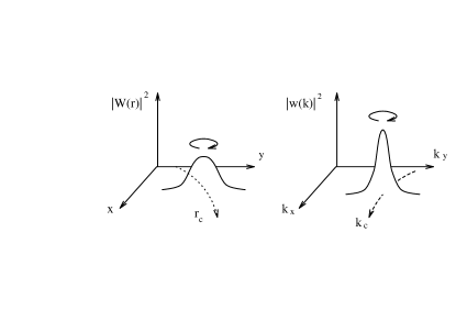
FIG. 1.: Schematic plots for the motion of wave packets in ${\bf r}$ and ${\bf k}$- space.

where we have used the identity[9]

$$\langle u({\bf k}^{\prime})|e^{i({\bf k}-{\bf k}^{\prime})\cdot{\bf r}}~{}i\frac{\partial}{\partial{\bf k}}|u({\bf k})\rangle=\delta({\bf k}-{\bf k}^{\prime})\langle u({\bf k})|i\frac{\partial}{\partial{\bf k}}|u({\bf k})\rangle_{\rm cell}.$$ (17)

The subscript means that the spatial integration is restricted to a magnetic unit cell. By defining

$$\mbox{\boldmath${\cal A}$}({\bf k})=i\langle u({\bf k})|\frac{\partial}{\partial{\bf k}}|u({\bf k})\rangle_{\rm cell},$$ (18)

Eq. (13) can be written as

$$\int d^{2}{\bf k}\left[w^{*}({\bf k})i\frac{\partial}{\partial{\bf k}}w({\bf k})+|w({\bf k})|^{2}\mbox{\boldmath${\cal A}$}({\bf k})\right]={\bf r}_{c}.$$ (19)

B Effective Lagrangian for a moving wave packet

The dynamics of a moving wave packet is governed by the following effective Lagrangian

$$L({\bf r}_{c},{\bf k}_{c},{\bf{\dot{r}}_{c}},{\bf{\dot{k}}_{c}})=\langle W|i\hbar\frac{\partial}{\partial t}|W\rangle-\langle W|H|W\rangle,$$ (20)

where $W$ is a wave packet centered at ${\bf r}_{c}$ and ${\bf k}_{c}$ in the presence of external electromagnetic fields (${\bf k}_{c}$ is treated as a generalized coordinate here). We can always choose a gauge such that the vector potential $\delta{\bf A}$ is locally gauged away at a chosen point ${\bf r}={\bf r}_{c}$. At this particular point, the moving wave packet $W$ is the same as the $W_{0}$ in Eq. (2.2).[10] The value of $W$ near ${\bf r}_{c}$ can be approximated as

$$W({\bf r})=e^{-ie/\hbar\delta{\bf A}({\bf r}_{c},t)\cdot{\bf r}}W_{0}({\bf r}).$$ (21)

First, we evaluate the energy of this wave packet, which is $\langle W|H|W\rangle=\langle W_{0}|H^{\prime}|W_{0}\rangle$, with

$$H^{\prime} = \frac{1}{2m}\left\{-i\hbar\frac{\partial}{\partial{\bf r}}+e{\bf A}_{0}({\bf r})+e\left[\delta{\bf A}({\bf r},t)-\delta{\bf A}({\bf r}_{c},t)\right]\right\}^{2}+V({\bf r})$$ (22)

$$\simeq H_{0}+\frac{e}{2m}\left\{\left[\delta{\bf A}({\bf r},t)-\delta{\bf A}({\bf r}_{c},t)\right]\cdot{\bf P}+{\rm h.c.}\right\}.$$ (23)

${\bf P}$ is the mechanical momentum operator corresponding to $H_{0}$. For simplicity, we choose the circular gauge for $\delta B$, which gives $\delta{\bf A}({\bf r},t)=-{\bf E}t+\frac{1}{2}\delta{\bf B}\times{\bf r}$, and leads to

$$H^{\prime}\simeq H_{0}+\frac{e}{2m}\delta{\bf B}\cdot{\bf L},$$ (24)

where ${\bf L}=({\bf r}-{\bf r}_{c})\times{\bf P}$ is the mechanical angular momentum of the wave packet about its center of mass. Therefore,

$$\langle W|H|W\rangle\simeq{\cal E}({\bf k}_{c})+\frac{e}{2m}\delta{\bf B}\cdot\langle W_{0}|{\bf L}|W_{0}\rangle.$$ (25)

The second term represents the energy correction due to magnetic moment of the wave packet. Notice that while a wave packet in an ordinary Bloch band does not rotate, a wave packet in a magnetic Bloch band usually does.

For the first term on the right hand side of Eq. (2.9), we have

$$\langle W_{0}|i\hbar\frac{\partial}{\partial t}|W_{0}\rangle$$ (26)

$$= \langle W_{0}|e\delta{\bf\dot{A}}({\bf r}_{c},t)\cdot{\bf r}|W_{0}\rangle+\int d^{2}{\bf k}~{}w^{*}({\bf k})i\hbar\frac{\partial}{\partial t}w({\bf k})$$ (27)

$$= e\delta{\bf\dot{A}}({\bf r}_{c},t)\cdot{\bf r}_{c}+\int d^{2}{\bf k}~{}|w({\bf k})|^{2}\hbar\frac{\partial}{\partial t}\gamma({\bf k},t)$$ (28)

$$\simeq e\delta{\bf\dot{A}}({\bf r}_{c},t)\cdot{\bf r}_{c}+\hbar\frac{\partial}{\partial t}\gamma({\bf k}_{c},t),$$ (29)

where $w({\bf k})\equiv|w({\bf k})|e^{-i\gamma({\bf k},t)}$. Up to terms of total time derivative, which have no effect on the dynamics, the last line can be written as

$$-e\delta{\bf A}\cdot{\bf\dot{r}}_{c}-\hbar{\bf\dot{k}}_{c}\cdot\frac{\partial}{\partial{\bf k}}_{c}\gamma({\bf k}_{c},t).$$ (30)

Using the condition in Eq. (19) and neglecting another term of total time derivative, we can write Eq. (30) as

$$-e\delta{\bf A}\cdot{\bf\dot{r}}_{c}+\hbar{\bf k}_{c}\cdot{\bf\dot{r}}_{c}+\hbar{\bf\dot{k}}_{c}\cdot{\mbox{\boldmath${\cal A}$}}({\bf k}_{c}).$$ (31)

Combining Eqs. (25) and (31), we have a final form for the effective Lagrangian (omitting subscript $c$)

$$L({\bf r},{\bf k},{\bf\dot{r}},{\bf\dot{k}})=-e\delta{\bf A}({\bf r},t)\cdot{\bf\dot{r}}+\hbar{\bf k}\cdot{\bf\dot{r}}+\hbar\mbox{\boldmath${\cal A}$}({\bf k})\cdot{\bf\dot{\bf k}}-E({\bf k}),$$ (32)

where $E({\bf k})\equiv{\cal E}({\bf k})+(e/2m)\delta{\bf B}\cdot{\bf L}({\bf k})$. Under a gauge transformation for ${\bf A}_{0}({\bf r})$, the Berry potential $\mbox{\boldmath${\cal A}$}({\bf k})$ will be changed by a term like $\partial_{{\bf k}_{0}}\chi({\bf k}_{0})$, and this will only change $L$ by a total time derivative. This is also true if a different gauge is chosen for $\delta{\bf B}$. Therefore, the dynamics is invariant under gauge transformation.

The dynamical equations in Eqs. (8) and (9) can be obtained straightforwardly from this Lagrangian by using the Euler-Lagrange equation. The relation between ${\bf\Omega}({\bf k})$ and $\mbox{\boldmath${\cal A}$}({\bf k})$ is

$${\bf\Omega}({\bf k})=\nabla\times\mbox{\boldmath${\cal A}$}({\bf k}),$$ (33)

which can also be written as ($z$-component)

$$\Omega({\bf k})=i\left({\langle\frac{\partial u_{n}}{\partial k_{1}}|\frac{\partial u_{n}}{\partial k_{2}}\rangle-\langle\frac{\partial u_{n}}{\partial k_{2}}|\frac{\partial u_{n}}{\partial k_{1}}\rangle}\right).$$ (34)

This is the familiar Berry curvature in the study of the quantum Hall effect.[11]

III Transport in magnetic Bloch bands

A Transport by an electric field

The next step is to combine the semiclassical equations with Boltzmann equation to study the transport properties of magnetic Bloch electrons. The Boltzmann equation is

$${\bf{\dot{r}}}\cdot\frac{\partial f}{\partial{\bf r}}+{\bf{\dot{k}}}\cdot\frac{\partial f}{\partial{\bf k}}=\left(\frac{\partial f}{\partial t}\right)_{\rm coll},$$ (35)

where $f=f({\bf r},{\bf k})$ is a distribution function. The effect of impurities is included in the collision term $\left(\partial f/\partial t\right)_{\rm coll}$. We use the relaxation time approximation to replace it by $-(f-f_{0})/\tau({\bf k})$. For a random distribution of delta impurities $v_{0}\sum_{i}\delta({\bf r}-{\bf r}_{i})$, the impurity scattering rate is

$$\tau({\cal E}_{F})^{-1}=\frac{\pi}{\hbar}\rho({\cal E}_{F})n_{i}v_{0}^{2},$$ (36)

where $n_{i}$ is the area density of impurities. This rate is proportional to the density of states $\rho({\cal E}_{F})$ at Fermi energy, which varies wildly with ${\cal E}_{F}$ because the energy spectrum is discrete. However, since the following calculation is confined to only one band, $\tau$ will be approximated by a constant.

The equations of motion of an electron subject to a uniform electric field are

$${\bf{\dot{r}}}=\frac{\partial{\cal E}({\bf k})}{\hbar\partial{\bf k}}+\frac{e}{\hbar}{\bf E}\times{\bf\Omega}({\bf k}),\ \ {\bf\dot{k}}=-e{\bf E},$$ (37)

where ${\cal E}({\bf k})$ is the reduced form of $E({\bf k})$ in the absence of $\delta B$. Substituting the expressions for ${\bf\dot{r}}$ and ${\bf\dot{k}}$ in Eq. (3.3) into Eq. (3.1), and setting $f=f_{0}$ on the left hand side of Eq. (3.1), we obtain

$$f=f_{0}-\tau\left(\frac{\partial{\cal E}}{\hbar\partial{\bf k}}\cdot\frac{\partial f_{0}}{\partial{\bf r}}+\frac{e}{\hbar}({\bf E}\times{\bf\Omega})\cdot\frac{\partial f_{0}}{\partial{\bf r}}-\frac{e}{\hbar}{\bf E}\cdot\frac{\partial f_{0}}{\partial{\bf k}}\right),$$ (38)

where $f_{0}$ is the distribution function in equilibrium. Electric current is given by

$${\bf J}=-e\int\frac{d^{2}{\bf k}}{(2\pi)^{2}}f{\bf\dot{r}}.$$ (39)

It can be decomposed into three parts, ${\bf J}^{\Omega}+{\bf J}^{\tau}+{\bf J}^{\mu}$, with the following definitions:

$${\bf J}^{\Omega} = -{\bf E}\times\frac{e^{2}}{\hbar}\int\frac{d^{2}{\bf k}}{(2\pi)^{2}}f_{0}{\bf\Omega}({\bf k}),$$ (40)

$${\bf J}^{\tau} = e^{2}\tau\int\frac{d^{2}{\bf k}}{(2\pi)^{2}}\left(-\frac{\partial f_{0}}{\partial{\cal E}}\right){\bf v_{b}}\left({\bf v_{b}}\cdot{\bf E}\right),$$ (41)

$${\bf J}^{\mu} = e\tau\int\frac{d^{2}{\bf k}}{(2\pi)^{2}}\left(-\frac{\partial f_{0}}{\partial{\cal E}}\right){\bf v}\left({\bf v}\cdot\frac{\partial\mu}{\partial{\bf r}}\right).$$ (42)

In these expressions, ${\bf v_{b}}$ is the velocity $\partial{\cal E}/\hbar\partial{\bf k}$ due to energy dispersion, and ${\bf v}$ is the total velocity in Eq. (3.3). The meaning of these currents is explained below.

First, ${\bf J}^{\Omega}$ is the Hall current. This is most evident considering a filled band with $f_{0}=1$. In this case, both ${\bf J}^{\tau}$ and ${\bf J}^{\mu}$ vanish, and only ${\bf J}^{\Omega}$ is nonzero. The integral of $\Omega({\bf k})$ over one magnetic Brillouin zone divided by $2\pi$ is always an integer, which is the topological Chern number discovered by Thouless et al. [11] Therefore we have

$${\bf J}^{\Omega}=-{\rm C}\frac{e^{2}}{h}{\bf E}\times{\hat{z}},\ \ ({\rm C}\in Z).$$ (43)

This formula represents the quantization of Hall current for a magnetic Bloch band.

Second, ${\bf J}^{\tau}$ is the diffusion current due to disorder scatterings. It can be put in the following form

$${\bf J}^{\tau}=e^{2}\int\frac{d^{2}{\bf k}}{(2\pi)^{2}}\left(-\frac{\partial f_{0}}{\partial{\cal E}}\right)\int^{\infty}_{0}dt~{}{\bf v_{b}}(t){\bf v_{b}}(0)\cdot{\bf E},$$ (44)

where ${\bf v_{b}}(t)\equiv e^{-t/\tau}{\bf v_{b}}(0)$ is the current relaxed by scatterings after time $t$. At very low temperature, it can be simplified to

$${\bf J}^{\tau}=e^{2}g({\cal E}_{F}){\bf\sf D}\cdot{\bf E},$$ (45)

where $g({\cal E}_{F})$ is the density of states at Fermi energy. ${\bf\sf D}\equiv\int_{0}^{\infty}dt\langle{\bf v_{b}}(t){\bf v_{b}}(0)\rangle$ is the diffusion tensor, and the angular bracket $\langle\ \rangle$ means averaging over the Fermi surface. [12]

Third, ${\bf J}^{\mu}$ is the current due to density gradient. It can be put in a form similar to ${\bf J}^{\tau}$ in Eq. (3.9) at low temperature, but with two changes: (1) The velocity ${\bf v_{b}}$ in ${\bf\sf D}$ is replaced by the total velocity ${\bf v}$ that includes the curvature term. (2) The driving force $e{\bf E}$ is replaced by $\partial\mu/\partial{\bf r}$. To evaluate this current, we need to know the explicit form of $\Omega({\bf k})$. This in general requires numerical calculation (see Sec. VI).

We remark that, even though the derivation of Eq. (3.8) is based on a uniform electric field, its validity goes beyond that. It is actually a kinetic formulation, first proposed by Chambers, that is also valid in the presence of a magnetic field (for magnetic Bloch bands, the magnetic field is $\delta B$).[13]

B Perturbation by an AC electric field

The semiclassical method is much simpler to use than full quantum mechanical approaches. This is most evident when the perturbation is changing in time. We illustrate this by considering a magnetic Bloch electron in an AC electric field. To simplify the discussion, we will neglect the effect of disorder and focus on the dynamics itself.

Assuming that a uniform electric field along the $x$ direction oscillates with a low frequency $\omega$, we then have

$${\bf{\dot{r}}} = \frac{\partial{\cal E}({\bf k})}{\hbar\partial{\bf k}}-\frac{e}{\hbar}E_{0}e^{i\omega t}\Omega({\bf k}){\hat{y}},$$ (46)

$$\hbar{\bf\dot{k}} = -eE_{0}e^{i\omega t}{\hat{x}}.$$ (47)

Considering a square lattice with the following energy spectrum

$${\cal E}({\bf k})=2\left[\cos(k_{1}a)+\cos(k_{2}a)\right],$$ (48)

and substituting the solution ${\bf k}(t)$ into the ${\bf\dot{r}}$ equation in (3.10), we have

$$\hbar{\dot{x}} = 2a\sin\left(\frac{eE_{0}a}{\hbar\omega}\sin(\omega t)-k_{0x}a\right)$$ (49)

$$\hbar{\dot{y}} = -2a\sin(k_{0y}a)-\frac{eE_{0}}{\hbar}\Omega({\bf k}(t))\cos(\omega t),$$ (50)

where $(k_{0x},k_{0y})$ is the initial value of ${\bf k}$. It is not difficult to see that after many cycles of oscillation, there is a net drift along the $x$ direction with average velocity

$$\langle{\dot{x}}\rangle=-\frac{2a}{\hbar}\sin(k_{0x}a)J_{0}(z),$$ (51)

where $J_{0}$ is the zeroth order Bessel function, and $z\equiv eE_{0}a/\hbar\omega$ is a ratio between two energy scales.[15] It can be seen that the original band transport velocity $-2a/\hbar\sin(k_{0x}a)$ is modified by $J_{0}(z)$ because of the AC field. The electron is immobile along the $x$ direction when $z$ is a zero of the Bessel function. This resembles the collapse of the usual Bloch band in the AC Wannier-Stark ladder problem.[16]

Finally, we comment that the use of semiclassical equations is based on the assumption that impurities do not alter the band structure. Therefore, the electron dynamics between collisions can be nicely described by Eqs. (8) and (9). This assumption is no longer valid when $q$ is large. In that case, disorder broadening tends to merge the subbands and wash out the fine structure. (This will be clearer after the discussion of hierarchical structure of the energy bands in Sec. V.) However, it was found that despite the energy spectrum has singular $B$ dependence, the density of states appears as a continuous function of the magnetic field. [14] Therefore, we divide total magnetic field $B$ into $B_{0}$ and $\delta B$, where $B_{0}$ is related to the band structure undestroyed by disorder, and $\delta B$ is a small perturbation. In this case, the semiclassical dynamics in the magnetic Bloch band of $B_{0}$, driven by $E$ and $\delta B$, will be employed in the Boltzmann equation.

IV Magnetic perturbation and hyperorbits

The usual Bloch electron will circulate around the Fermi surface along a constant energy contour in the presence of a magnetic field. It is well-known that the quantization of cyclotron orbits leads to the famous de Haas-Van Alphen effect. In this section, we study a similar type of cyclotron motion in magnetic Bloch bands. It will be seen that this investigation yields very fruitful results. In particular, it offers a very simple explanation for the complex Hofstadter spectrum, which will be shown in Sec. V and Sec. VI.

A General properties of hyperorbits

Combining the two equations in (3.3), we can eliminate ${\bf\dot{r}}$ to obtain

$$\hbar{\bf\dot{k}}=-eZ_{\delta B}({\bf k})\frac{\partial E({\bf k})}{\hbar\partial{{\bf k}}}\times\delta{\bf B}.$$ (52)

where $Z_{\delta B}({\bf k})\equiv(1+\Omega({\bf k})\delta Be/\hbar)^{-1}$ is a curvature correction factor. This equation determines the trajectories of magnetic Bloch electrons in ${\bf k}$-space. It is not difficult to see that ${\bf k}$ moves along a constant energy contour of $E({\bf k})$ (which is slightly different from ${\cal E}({\bf k})$). In a classical picture, it is the drifting-center trajectory of the tighter cyclotron orbit formed from $B_{0}$. However, we have to emphasize that, the existence of hyperorbits is of quantum origin and cannot be explained classically. To differentiate them from the usual orbits of Bloch electrons, we will call them ’hyperorbits’. [17] The hyperorbit in real space is derived from ${\bf\dot{r}}={\bf\dot{k}}\times{\hat{z}}(\hbar/e\delta B)$, which is the ${\bf k}$-orbit rotated by $\pi/2$ and scaled by the factor $\hbar/e\delta B$. It is also possible to define an effective cyclotron mass according to its frequency. However, this frequency will be very sensitive to its energy if the magnetic Bloch band is narrow, which is usually the case.

There are several ways to verify the existence of hyperorbits. One way is through the measurement of magnetoresistance oscillation that originates from the quantization of hyperorbits. This oscillation has a much shorter period than the usual de Haas-van Alphen oscillation because the effective magnetic field $\delta B$ is much smaller. The other way of verifying it is by using an electron focusing device to detect its real space orbit.[18] This method has been used to map out the shape of a Fermi surface by measuring the shape of cyclotron orbits.[19] Another possible approach is to observe the ultrasonic absorption spectrum of the sample. The energy of an ultrasonic wave will be absorbed when it is in resonance with the hyperorbits. Similar method has been used to detect the existence of composite fermions in half-filled quantum Hall systems.[20]

B Quantization of hyperorbits

In a previous paper, we have derived the quantization condition using Lagrangian formulation combined with path integral method.[7] Here, it will be rederived using a slightly different approach. Substituting ${\bf\dot{r}}={\bf\dot{k}}\times{\hat{z}}(\hbar/e\delta B)$ into the Lagrangian in Eq. (2.17), we will obtain an effective Lagrangian for the quasimomentum ${\bf k}$,

$$L({\bf k},{\bf{\dot{k}}})=\frac{\hbar^{2}}{e\delta B}(k_{1}{\dot{k}}_{2}-k_{2}{\dot{k}}_{1})+\hbar{\mbox{\boldmath{${\cal A}$}}}\cdot{{\bf\dot{k}}}-E({\bf k}).$$ (53)

It can be easily shown that Eq. (4.1) does follow from this $L$. The generalized momentum for coordinate ${\bf k}$ is equal to

$$\mbox{\boldmath$\pi$}=\frac{\partial L}{\partial{\bf\dot{k}}}=-\frac{\hbar^{2}}{2e\delta B}{\bf k}\times{\hat{z}}+\hbar\mbox{\boldmath${\cal A}$}({\bf k}).$$ (54)

This leads to the following effective Hamiltonian

$$H({\bf k},\mbox{\boldmath$\pi$})\equiv\mbox{\boldmath$\pi$}\cdot{\bf\dot{k}}-L({\bf k},{\bf\dot{k}})=E({\bf k}).$$ (55)

Notice that because $H$ does not depend on $\pi$, the coordinate ${\bf k}$ will be a constant of motion and the dynamics is trivial. A Hamiltonian that gives correct dynamics will be given in Appendix A. Since it is not central to our derivation, we will not discuss it here.

The quantization of hyperorbits is given by $\oint\mbox{\boldmath$\pi$}\cdot d{{\bf k}}=(m+\gamma)h$, where $m$ is a non-negative integer and $\gamma$ will be taken to be $1/2$. It leads to area quantization in ${\bf k}$-space

$$\frac{1}{2}\oint_{C_{m}}({\bf k}\times d{\bf k})\cdot{\hat{z}}=2\pi\left(m+\frac{1}{2}-\frac{\Gamma(C_{m})}{2\pi}\right)\frac{e\delta B}{\hbar},$$ (56)

where

$$\Gamma(C_{m})=\oint_{C_{m}}{\mbox{\boldmath{${\cal A}$}}}\cdot d{\bf k}$$ (57)

is the Berry phase for orbit $C_{m}$. The orientation of $C_{m}$ is chosen such that the sign of the area on the left hand side of Eq. (4.5) equals the sign of $\delta B$.

The total number of hyperorbits in a MBZ is determined by requiring the area of the outer-most orbit be smaller than the area of a MBZ. Assume the flux before perturbation is $B_{0}a^{2}=p/q$, then the number of hyperorbits in a MBZ is equal to $\left|1/(q\delta\phi)+\sigma\right|$,[7] where $\delta\phi\equiv\delta Ba^{2}e/h$, and $\sigma$ is the Hall conductivity of the parent band. These hyperorbits are the lowest order approximation to the split energy subbands. They will be broadened by tunnelings between degenerate orbits. Since the MBZ is $q$-fold degenerate, the above number has to be divided by $q$ to get the actual number of daughter bands,

$$D=\frac{|1/(q\delta\phi)+\sigma|}{q}.$$ (58)

This formula is essential in understanding the splitting pattern of the Hofstadter spectrum.

The Hall conductivity for a subband can be calculated in the following way: In the presence of both $\bf E$ and $\delta{\bf B}$, the velocity of a magnetic Bloch electron consists of two parts,[1]

$${\bf{\dot{r}}}=\frac{\hbar}{e\delta B}{\bf{\dot{k}}}\times{\hat{z}}+\frac{{\bf E}\times{\hat{z}}}{\delta B}.$$ (59)

The first term is the velocity of revolution, and the second term is the velocity of drifting along ${\bf E}\times{\bf B}$ direction. The current density for a filled subband is

$${\bf J}=-\int d^{2}{\bf k}\frac{\hbar}{\delta B}{\bf{\dot{k}}}\times{\hat{z}}-e\int d^{2}{\bf k}\frac{{\bf E}\times{\hat{z}}}{\delta B}.$$ (60)

The first integral is zero for a closed orbit. Therefore, the Hall conductivity is obtained from the drifting term, which leads to $\sigma_{yx}({\rm or\ simply}\ \sigma)=\rho e/\delta B$, where $\rho$ is the electron density per unit area. This will be used in the next section to determine the Hall conductivities for subbands in the Hofstadter spectrum.

V The Hofstadter spectrum

A Hierarchical structure of the spectrum

The discussion in the preceding section presumes that we know $\delta B$. But this is not apparent if the magnetic field $B$ is homogeneous. In this case, we can still divide it into two parts, but where is the dividing point between $B_{0}$ and $\delta B$? A natural way of dividing $B$ (or $\phi$) is to write it as a continuous fraction,

$$\phi={1\over\displaystyle f_{1}+{1\over\displaystyle f_{2}+{1\over\displaystyle{{f_{3}+\cdots}}}}},$$ (61)

and truncate it according to the accuracy we need. The $r$-th order approximation of $\phi$ will be written as $p_{r}/q_{r}$.[21] For example, if $\phi=1/(2+\sqrt{2})$, we will have $p_{1}/q_{1}=1/3,\ p_{2}/q_{2}=2/7,\ p_{3}/q_{3}=5/17\cdots$ etc, which are truncations of

$$\frac{1}{2+\sqrt{2}}={1\over\displaystyle 3+{1\over\displaystyle 2+{1\over\displaystyle{{2+\cdots}}}}}.$$ (62)

The $q_{r}$’s satisfy the following recursion relation

$$q_{r+1}=f_{r+1}q_{r}+q_{r-1},$$ (63)

which relates the number of subbands at neighboring orders. There is also a relation between $p$’s and $q$’s,

$$p_{r+1}q_{r}-p_{r}q_{r+1}=(-1)^{r}.$$ (64)

It follows that the extra magnetic flux between the $r$-th order and the $(r+1)$-th order truncation is

$$\delta\phi_{r}=\frac{p_{r+1}}{q_{r+1}}-\frac{p_{r}}{q_{r}}=\frac{(-1)^{r}}{q_{r+1}q_{r}}.$$ (65)

Since the sign of $\delta\phi_{r}$ alternates from one order to the next, the direction of $\delta B$ also alternates.[22]

Notice that for a chosen fraction $p_{r}/q_{r}$, the size of a MBZ is fixed. Without perturbation from the part that is truncated away, a wave packet will move on a straight line. The trajectory is curved because of $\delta\phi_{r}$. Higher the order approximation we use, smaller the $\delta\phi$ gets and larger the radius of the hyperorbit becomes. In the ideal case, without any complications due to disorder, thermal broadening $\cdots$ etc, we expect there will be a hierarchical structure of hyperorbits due to different orders of approximation. This structure finds its correspondence in the hierarchical structure of the Hofstadter spectrum.[23] (Fig. 2)

FIG. 2.: Hofstadter spectrum for a square lattice generated from a tight-binding model ($q\leq 60$). Only the $\phi\leq 1/2$ part is shown since the spectrum is symmetric with respect to $\phi=1/2$.

B Distribution of Hall conductivities and splitting of energy bands

A magnetic Bloch band carries quantized Hall current, and this current will redistribute among daughter bands in such a way that the total Hall current for subbands equals the original current.[24] We will call this the “sum rule”. The current distribution among subbands, which is also quantized in each subband, was obtained by Thouless et al.[11] In their famous paper, they found that the subband Hall conductivities are the integer-valued solutions of the Diophantine equation. Here we show that semiclassical dynamics offers an alternative and very heuristic solution to this problem. The Hall conductivities calculated will be used in Eq. (4.7) to calculate the number of magnetic subbands after splitting.

The general expression for the Hall conductivity of a “closed” subband is $\sigma=\rho e/\delta B$ (see Eq. (4.9) and below). Therefore, $\sigma$ can be determined if $\rho$ and $\delta B$ are known. Consider a subband at the $r$-th order of splitting. Since all subbands at this level share the same number of states, each subband will have $\rho_{r}=\rho_{0}/q_{r}$, where $\rho_{0}$ is the density of states for the original Bloch band. The perturbation field for a subband at this level is $\delta B_{r}=h\delta\phi_{r-1}/(ea^{2})$. Therefore, we have

$$\sigma^{\rm close}_{r}=\frac{e\rho_{r}}{\delta B_{r}}=(-1)^{r-1}q_{r-1},\ ({\rm in\ units\ of}\ e^{2}/h).$$ (66)

(Since $\sigma_{1}=1$ for a closed subband at the first level, $q_{0}$ will be set to one .) We have to emphasize that, Eq. (5.6) is valid for every closed subbands at the $r$-th order. Combining Eq. (4.7) with (5.6), we can determine the number of daughter bands being split from a $r$-th order parent band, which is

$${\cal D}^{\rm close}_{r} = \frac{|(-1)^{r}q_{r+1}+\sigma_{r}^{\rm close}|}{q_{r}}$$ (67)

$$= f_{r+1}.$$ (68)

FIG. 3.: Schematic plots of the constant energy contours in the reduced MBZ of a square lattice and a triangular lattice. Dashed lines are the open orbits.

The Hall conductivity for an open subband is more difficult to obtain. It requires the knowledge of the exact ${\bf k}$-trajectory to figure out the first integral in Eq. (4.9). However, for a square or a triangular lattice, there is an easier way of calculating it. This is so because, there is only one open orbit in every MBZ for either lattice (see Fig. 3). Therefore, there is only one open daughter band for every parent band. Its Hall conductivity can be figured out by using the “sum rule”:

$$\sigma_{\rm parent}=\sum\sigma_{\rm daughter}.$$ (69)

For example, at the first order, we have $\sigma_{1}^{\rm open}=\sigma_{0}-(f_{1}-1)\sigma_{1}^{\rm close}=-(f_{1}-1)$, where $\sigma_{0}=0$ since it is a Bloch band at the very beginning. For $r\geq 2$, the Hall conductivity of an open daughter band at the $r$-th order is

$$\sigma^{\rm open}_{r} = \sigma_{r-1}^{\rm close}-(f_{r}-1)\sigma_{r}^{\rm close}$$ (70)

$$= (-1)^{r-2}q_{r-2}-(f_{r}-1)(-1)^{r-1}q_{r-1}$$ (71)

$$= (-1)^{r-1}q_{r-1}+(-1)^{r}q_{r},$$ (72)

where we have assumed that its parent is a ’closed’ band. Using Eq. (4.7), we see that this open band (now as a parent) will split into

$${\cal D}^{\rm open}_{r}=f_{r+1}+1$$ (73)

subbands under perturbation. It can be shown that the same result as Eq. (5.9) is obtained if its parent is an ’open’ band (with $f_{r}+1$ daughters). This checks the consistency of this calculation. It is clear that the extra splitting of one subband from each open parent band (there are $q_{r-1}$ of them) accounts for the extra $q_{r-1}$ in the recursion relation Eq. (63)

We give one example to demonstrate the use of these rules. Consider a square lattice with $\phi=1/(2+\sqrt{2})$. Because $\sigma_{1}^{\rm close}=1$, and $\sigma_{1}^{\rm open}=-2$, the distribution of $\sigma$’s for the three subbands at the first order is

$$\mbox{\boldmath$\sigma_{\rm 1}$}=(1,-2,1).$$ (74)

where we have put $\sigma_{1}^{\rm open}$ in the middle since for a square lattice the open subband is located at the center of a parent band (Fig. 3).

These three bands will be split into seven subbands due to the extra flux $\delta\phi_{1}=p_{2}/q_{2}-p_{1}/q_{1}=2/7-1/3$. Since $f_{2}=2$, the pattern of splitting will be, according to Eqs. (5.7) and (5.10),

$$\mbox{\boldmath${\cal D}_{\rm 1}$}=(2,3,2).$$ (75)

Furthermore, since $\sigma^{\rm close}_{2}=-3$ and $\sigma^{\rm open}_{2}=4$ according to Eqs. (5.6) and (5.9), the Hall conductivity distribution is [25]

$$\mbox{\boldmath$\sigma_{\rm 2}$}=(-3,4,-3,4,-3,4,-3).$$ (76)

Consequently, we have

$$\mbox{\boldmath${\cal D}_{\rm 2}$}=(2,3,2,3,2,3,2).$$ (77)

The Hall conductivities we just obtained are the same as those derived from the Diophantine equation. Actual pattern of splitting is shown in Fig. 4 for comparison. The distribution in Fig. 4 for the left (or right) five subbands in Eq. (5.14) appears to be $(2,1,2)$, instead of $(2,3)$ (or $(3,2)$). However, closer examination reveals that the left (right) three subbands actually come from the same parent. In fact, slight asymmetry in the distribution is inevitable because when $\phi$ is changed by a small amount, an electron state cannot suddenly jump out of the band edge to the middle of a gap.

Eqs. (5.6)–(5.10) also apply to a triangular lattice. The only difference is that $\sigma_{\rm open}$ no longer locates at the center of a parent band. Given the same $\phi=1/(2+\sqrt{2})$, we now have

$$\sigma_{\rm 1} = (1,1,-2)$$ (78)

$${\cal D}_{\rm 1} = (2,2,3)$$ (79)

$$\sigma_{\rm 2} = (4,-3,-3,4,4,-3,-3)$$ (80)

$${\cal D}_{\rm 2} = (3,2,2,3,3,2,2).$$ (81)

This again conforms with the actual spectrum and the solutions of the Diophantine equation with subsidiary constraints suitable for a triangular lattice.[26]

FIG. 4.: Pattern of energy splitting for $\phi$ in Eq. (5.2). Different orders of approximation give 3, 7, and 17 subbands respectively.

VI Calculations of energy spectrum, curvature, magnetic moment, and cyclotron energy

In this section, we give detailed calculations of ${\cal E}_{n}({\bf k})$, $\Omega_{n}({\bf k})$, and $L_{n}({\bf k})$. They are used in calculating the cyclotron energies using the quantization formula Eq. (56). The cyclotron energies will be used to estimate the subband energies in the Hofstadter spectrum. In doing so, we not only presume the one-band approximation (on which Fig. 2 is based), but also neglect the inter-orbit transitions that broaden (and may slightly shift) the energy levels. The latter approximation leads to negligible error if the bandwidths under consideration are very small. Similar calculations have been done by Wilkinson, and his results have been very successful.[27] However, we believe that the approach proposed here is conceptually simpler, and is easier to generalize to other types of lattices.

A Calculation of energy spectrum for parent bands

The following calculation is based on the tight-binding model. We will only give a very brief explanation of this approach. For more details, we request readers to refer to Ref. (29). In the tight-binding approximation, a Bloch state is expanded as (for $\phi=p/q$)

$$\Psi({\bf k})=\sum_{l=1}^{q}a_{l}({\bf k})\psi_{l}({\bf k}),$$ (82)

where ${\bf k}$ is restricted to a reduced MBZ. The basis $\psi_{l}({\bf k})$ is defined to be $\psi(k_{1}+2\pi\phi l,k_{2})$, where $\psi({\bf k})$ is a Bloch state before the magnetic perturbation. A tight-binding Hamiltonian in the absence of $\delta B$, when being expressed on the basis of $\psi_{l}$, is a $q\times q$ matrix (the lattice constant $a$ is set to one.)

$$H_{l^{\prime},l}=-\left(\begin{array}[]{cccccc}\cos(k_{1}+2\pi/q)&e^{ik_{2}}&0&\cdot&0&e^{-ik_{2}}\\ e^{ik_{2}}&\cos(k_{1}+4\pi/q)&e^{ik_{2}}&\ddots&\ddots&0\\ 0&e^{ik_{2}}&\ddots&\ddots&\ddots&\cdot\\ \cdot&\ddots&\ddots&\ddots&e^{ik_{2}}&0\\ 0&\ddots&\ddots&e^{ik_{2}}&\cos(k_{1}+(q-1)\frac{2\pi}{q})&e^{ik_{2}}\\ e^{-ik_{2}}&0&\cdot&0&e^{ik_{2}}&\cos(k_{1})\\ \end{array}\right).$$ (83)

${\cal E}_{n}({\bf k})$ and $a^{n}_{l}({\bf k})$ are nothing but the eigenvalues and eigenvectors of this matrix. For example, if $p/q=1/3$, then a straightforward calculation shows that the ${\cal E}_{n}({\bf k})$’s are solutions of the following characteristic equation,

$$-{\cal E}^{3}+6{\cal E}=2\left[\cos(3k_{1})+\cos(3k_{2})\right].$$ (84)

There are three roots for each ${\bf k}$, and variation of ${\bf k}$ over the MBZ leads to the three energy bands for $\phi=1/3$ (see Fig. 2). It is not difficult to see that the band edges are located at (from high to low) ${\cal E}_{1}({\bf g}),{\cal E}_{1}({\bf 0}),{\cal E}_{2}({\bf 0}),{\cal E}_{2}({\bf g}),{\cal E}_{3}({\bf g})$, and ${\cal E}_{3}({\bf 0})$, where ${\bf g}=(\pi/3,\pi/3)$.

B Calculation of Berry curvature

To calculate the Berry curvature in Eq. (34), we need to know the eigenvectors of $H_{l^{\prime}l}$. Before doing that, we will try to rewrite Eq. (34) in a form suitable for the tight-binding calculation. First, we insert a complete state $\sum_{n^{\prime}}|u_{n^{\prime}}\rangle\langle u_{n^{\prime}}|$ inside the dot products that appear in Eq. (34). Since we are using the one-band approximation, $n^{\prime}$ only runs through subbands in the same parent band, and

$$\Omega_{n}({\bf k})=i\sum_{n^{\prime}=1}^{q}\ {}^{\prime}\left[{\langle\frac{\partial u_{n}}{\partial k_{1}}|u_{n^{\prime}}\rangle\langle u_{n^{\prime}}|\frac{\partial u_{n}}{\partial k_{2}}\rangle-{\rm c.c.}}\right],$$ (85)

where we have dropped a term with $n^{\prime}=n$ since $\langle u_{n}|\partial/\partial{\bf k}|u_{n}\rangle$ is purely imaginary and does not contribute to the curvature. With the help of the identity

$$\langle u_{n^{\prime}}|\frac{\partial}{\partial{\bf k}}|u_{n}\rangle=\frac{\langle u_{n^{\prime}}|\frac{\partial\tilde{H}}{\partial{\bf k}}|u_{n}\rangle}{{\cal E}_{n^{\prime}}-{\cal E}_{n}},$$ (86)

where $\tilde{H}\equiv e^{-i{\bf k}\cdot{\bf r}}He^{i{\bf k}\cdot{\bf r}}$ (this and the following $H$’s are the unperturbed Hamiltonian in Eq. (1.3); the subscript ’0’ is dropped for brevity), we can rewrite Eq. (6.4) in the form

$$\Omega_{n}({\bf k})=i\sum_{n^{\prime}}\ ^{\prime}\left[\frac{\langle u_{n}|\frac{\partial\tilde{H}}{\partial k_{1}}|u_{n^{\prime}}\rangle\langle n_{n^{\prime}}|\frac{\partial\tilde{H}}{\partial k_{2}}|u_{n}\rangle}{({\cal E}_{n^{\prime}}-{\cal E}_{n})^{2}}-{\rm c.c.}\right].$$ (87)

Expanding $u_{n}$ by $\tilde{\psi}_{l{\bf k}}({\bf r})$, which is defined to be $e^{-i{\bf k}\cdot{\bf r}}\psi_{l{\bf k}}({\bf r})$, we have

$$\langle u_{n^{\prime}}|\frac{\partial\tilde{H}}{\partial{\bf k}}|u_{n}\rangle = \sum_{l^{\prime},l}a^{n^{\prime}*}_{l^{\prime}}a^{n}_{l}\langle\tilde{\psi}_{l^{\prime}}|\frac{\partial\tilde{H}}{\partial{\bf k}}|\tilde{\psi}_{l}\rangle$$ (88)

$$= \sum_{l^{\prime},l}a^{n^{\prime}*}_{l^{\prime}}a^{n}_{l}\frac{\partial}{\partial{\bf k}}\langle\tilde{\psi}_{l^{\prime}}|\tilde{H}|\tilde{\psi}_{l}\rangle$$ (89)

$$+ ({\cal E}_{n}-{\cal E}_{n^{\prime}})\sum_{l^{\prime},l}a^{n^{\prime}*}_{l^{\prime}}a^{n}_{l}\langle\tilde{\psi}_{l^{\prime}}|\frac{\partial\tilde{\psi}_{l}}{\partial{\bf k}}\rangle.$$ (90)

The inner product $\langle\tilde{\psi}_{l^{\prime}}|\partial\tilde{\psi}_{l}/\partial{\bf k}\rangle$ is zero for a Bloch state in the absence of a magnetic field. Therefore,

$$\langle u_{n^{\prime}}|\frac{\partial\tilde{H}}{\partial{\bf k}}|u_{n}\rangle=\sum_{l}a^{n^{\prime}*}_{l}a^{n}_{l}\frac{\partial H_{l^{\prime},l}}{\partial{\bf k}}.$$ (91)

Beyond this stage, the calculation is straightforward since we only need to calculate $a^{n}_{l}$ from Eq. (83) and combine Eqs. (87) and (6.8) to obtain $\Omega_{n}({\bf k})$.

Again we choose a simple fraction $p/q=1/3$ and calculate the Berry curvature distributions for the three magnetic subbands. The result is shown in Fig. 5, in which the range of ${\bf k}$ vector is one reduced MBZ (the basic unit of repetition). Note that the curvature tends to concentrate on four inner band edges because the electron states near inner gaps are changed the most from the original Bloch states that have zero Berry curvature. The curvatures from the three bands cancel locally, that is

$$\sum_{n=1}^{3}\Omega_{n}({\bf k})=0,\ \ \forall\ {\bf k}.$$ (92)

This is in general true for any $q$ and can be easily proved from Eq. (87). Finally, integration of $\Omega_{n}({\bf k})$ over a MBZ divided by $2\pi$ gives us integers $(1,-2,1)$. These are indeed the Chern numbers we expected (see Eq. (5.11)).

FIG. 5.: Distributions of Berry curvature $\Omega_{n}({\bf k})$ (in units of $e^{2}/h$). $\Omega_{1}({\bf k})$ is equal to $\Omega_{3}({\bf k})$ shifted by $(\pi/3,\pi/3)$

C Calculation of magnetic moment

The self-rotating angular momentum of the wave packet $\langle{\bf L}\rangle_{n{\bf k}}$ in Eq. (2.13) can be written in a from that is more tractable for calculation:

$$L_{n}({\bf k})=i\frac{m}{\hbar}\left[\langle\frac{\partial u_{n}}{\partial k_{1}}|\tilde{H}-{\cal E}_{n}|\frac{\partial u_{n}}{\partial k_{2}}\rangle-{\rm c.c.}\right].$$ (93)

Derivation of this formula is given in Appendix B. Eq. (93) can also be rewritten as

$$L_{n}({\bf k})=i\frac{m}{\hbar}\sum_{n^{\prime}}\ ^{\prime}\left[\frac{\langle u_{n}|\frac{\partial\tilde{H}}{\partial k_{1}}|u_{n^{\prime}}\rangle\langle n_{n^{\prime}}|\frac{\partial\tilde{H}}{\partial k_{2}}|u_{n}\rangle}{{\cal E}_{n^{\prime}}-{\cal E}_{n}}-{\rm c.c.}\right].$$ (94)

Derivation of Eq. (94) is very similar to the derivation of Eq. (87). The only change is that the extra factor of $\tilde{H}-{\cal E}_{n}$ in the numerator cancels a ${\cal E}_{n^{\prime}}-{\cal E}_{n}$ in the denominator.

$L_{n}({\bf k})$ can be readily calculated by combining Eq. (91) with Eq. (94). The result is shown in Fig. 6 (again for $\phi=1/3$). Similar to the distribution of $\Omega_{n}({\bf k})$, $L_{n}({\bf k})$ also has peaks near inner band edges. The total magnetizations from all three bands cancel each other. However, unlike the curvature, they do not cancel locally at each ${\bf k}$ point.

We remark that this magnetization energy first appeared in a paper by Kohn[2]. Their objective was to study the effective Hamiltonian for Bloch electrons in a weak electromagnetic field. This term is in general zero for Bloch bands, but can be nonzero in the presence of spin-orbit interaction. In the latter case, it contributes an extra g-factor to Bloch electrons.[29] An expression that is the same as the right hand side of Eq. (93) has also been obtained by Rammal and Bellissard.[30] Without the $m/\hbar$ factor (and apart from a factor of two), it is called the Rammal-Wilkinson form.

FIG. 6.: Distributions of angular momentum $L_{n}({\bf k})$ (in units of $2m/\hbar$).

D Calculation of cyclotron energy

After obtaining ${\cal E}_{n}({\bf k})$, $\Omega_{n}({\bf k})$, and $L_{n}({\bf k})$, we can determine the cyclotron energies according to the quantization formula Eq. (56). In the following example, we add $\delta\phi=-1/201$ to $\phi=1/3$. This gives $\phi^{\prime}=22/67=1/(3+1/22)$. According to the simple rules derived in previous section, the original magnetic bands are expected to split to 22, 23, and 22 subbands respectively. In Table II, we compare the exact spectrum with the quantized cyclotron energies. Only part of the subbands from the parent band in the middle are shown. We show two numbers (for two band edges) in the first row when the bandwidth for $E_{\rm Hofst}$ is larger than $10^{-4}$. The $E_{\rm cyclo}$’s in the second row are obtained by fine-tuning the path $C_{m}$ in Eq. (56), with uncertainty on the order of $10^{-4}$. It can be seen that the match between $E_{\rm cyclo}$ and $E_{\rm Hofst}$ is quite satisfying. We have done calculations for subbands from other parent bands, and they also show similar accuracy.

Notice that the energy levels from fractions like $\phi=1/f$ are broadened cyclotron levels in an ordinary Bloch band. They do not split from a magnetic parent band. In this case $\Omega_{n}({\bf k})$ and $L_{n}({\bf k})$ are zero, and Eq. (56) reduces to the usual Onsager quantization formula. Numerical result based on this simplified formula for the cyclotron energies also agrees very well with the positions of subbands in Fig. 2.

VII Summary

Electron states in a lattice subject to a homogeneous magnetic field satisfy magnetic translation symmetry and have band-like energy spectrum similar to the usual Bloch band. However, to our knowledge, the semiclassical dynamics of magnetic Bloch electrons has never been an explicit subject. One reason is that the observation of band-splitting remains an experimental challenge to date; the other reason might be due to the fact that magnetic Bloch bands, unlike Bloch bands, can be changed easily by varying an external magnetic field. However, our study has shown that the inquiry of magnetic Bloch bands can be very rewarding in itself. Major findings in this paper are summarized below:

The Berry curvature of magnetic bands plays a crucial role in the dynamics. It gives electrons an extra velocity in the direction of ${\bf E}\times{\bf B}$, and this term directly relates to the quantization of Hall conductivity. This semiclassical dynamics, combined with the Boltzmann equation, is used to study electron transport in a DC or AC electric field.

In the presence of $\delta B$, the energy dispersion $E({\bf k})$ is shifted from the usual band energy because of the non-zero magnetic moment. Similar to usual Bloch electrons, magnetic Bloch electrons execute cyclotron motion on the constant energy surface of $E({\bf k})$. However, the quantization condition for cyclotron orbits has to be modified from the usual Onsager condition because of the Berry phase. Based on this modified formula, we obtain a simple rule that calculates the number of daughter bands for every parent band in the Hofstadter spectrum. Furthermore, a fairly heuristic explanation for the distribution of Hall conductivities is given using the picture of cyclotron orbit drifting.

These quantized orbits are closely related to the energy bands in the Hofstadter spectrum. We give detailed numerical calculations for $\Omega_{n}({\bf k})$ and $L_{n}({\bf k})$ based on the tight-binding model for the case of $\phi=1/3$. They are used in the calculation of cyclotron energies using the quantization condition, and the result is in very good agreement with the actual spectrum. This shows that the complex pattern of the Hofstadter spectrum is nothing more than the broadened cyclotron energy spectrum in magnetic Bloch bands.

A

Note that there is no ${\bf\dot{k}}$ dependence in $\pi$ (because there is no kinetic energy term ${\bf\dot{k}}^{2}$ in $L({\bf k},\dot{\bf k})$). In this case, it is more pertinent to treat Eq. (4.3) as a constraint on the variables ${\bf k}$ and $\pi$,

$$\mbox{\boldmath$\theta$}({\bf k},\mbox{\boldmath$\pi$})\equiv\mbox{\boldmath$\pi$}+\frac{\hbar^{2}}{2e\delta B}{\bf k}\times{\hat{z}}-\hbar\mbox{\boldmath${\cal A}$}({\bf k})\simeq 0.$$ (A1)

Strictly speaking, this constraint cannot be used before obtaining the equations of motion, therefore we use $\simeq$ to distinguish it from a real identity.[31] A general Hamiltonian for a system with constraints is given by,

$$H^{*}({\bf k},\mbox{\boldmath$\pi$})=H({\bf k},\mbox{\boldmath$\pi$})+{\mbox{\boldmath$\lambda$}}\cdot{\rm\mbox{\boldmath$\theta$}}=E({\bf k})+{\mbox{\boldmath$\lambda$}}\cdot{\rm\mbox{\boldmath$\theta$}},$$ (A2)

where $\mbox{\boldmath$\lambda$}=(\lambda_{1},\lambda_{2})$ are arbitrary functions of ${\bf k}$ and $\pi$. The dynamical equations for this new Hamiltonian are

$${\bf\dot{k}} = \frac{\partial H^{*}}{\partial\mbox{\boldmath$\pi$}}=\mbox{\boldmath$\lambda$}$$ (A3)

$${\bf\dot{\mbox{\boldmath$\pi$}}} = -\frac{\partial H^{*}}{\partial{\bf k}}=-\frac{\partial E}{\partial{\bf k}}+\frac{\hbar^{2}}{2e\delta B}\mbox{\boldmath$\lambda$}\times{\hat{z}}+\hbar\sum_{i}\lambda_{i}\frac{\partial{\cal A}_{i}}{\partial{\bf k}},$$ (A4)

where we have discarded a term $\partial\mbox{\boldmath$\lambda$}/\partial{\bf k}\cdot{\mbox{\boldmath$\theta$}}=0$. According to Eq. (4.3), we should also have

$${\bf\dot{\mbox{\boldmath$\pi$}}}=-\frac{\hbar^{2}}{2e\delta B}{\bf\dot{k}}\times{\hat{z}}+\hbar\sum_{i}{\dot{k}}_{i}\frac{\partial{\mbox{\boldmath{${\cal A}$}}}}{\partial k_{i}}.$$ (A5)

Equating (A3) to (A4), and replacing $\lambda$ by ${\bf\dot{k}}$, we will get Eq. (4.1).

B

We will rewrite the angular momentum of a wave packet in Eq. (2.13) in terms of magnetic Bloch functions. By defining $\tilde{w}({\bf k})=e^{i{\bf k}\cdot{\bf r}_{c}}w({\bf k})$, we have

$${\bf L}_{n}({\bf k}_{c}) = \int d^{2}{\bf k}^{\prime}\int d^{2}{\bf k}\ w^{*}({\bf k}^{\prime})w({\bf k})\langle\Psi_{n}({\bf k}^{\prime})|({\bf r}-{\bf r}_{c})\times{\bf P}|\Psi_{n}({\bf k})\rangle$$ (B1)

$$= \int d^{2}{\bf k}^{\prime}\int d^{2}{\bf k}\ \tilde{w}^{*}({\bf k}^{\prime})\tilde{w}({\bf k})\langle u_{n}({\bf k}^{\prime})|e^{i({\bf k}-{\bf k}^{\prime})\cdot({\bf r}-{\bf r}_{c})}({\bf r}-{\bf r}_{c})\times{\bf\tilde{P}}({\bf k})|u_{n}({\bf k})\rangle,$$ (B2)

where ${\bf\tilde{P}}$ is the momentum operator on the $|u_{n}\rangle$ basis. Since

$${\bf\tilde{P}}({\bf k})|u_{n}({\bf k})\rangle=\sum_{n^{\prime}}|u_{n^{\prime}}({\bf k})\rangle\langle u_{n^{\prime}}({\bf k})|{\bf\tilde{P}}({\bf k})|u_{n}({\bf k})\rangle,$$ (B3)

and

$$\langle u_{n}({\bf k}^{\prime})|e^{i({\bf k}-{\bf k}^{\prime})\cdot({\bf r}-{\bf r}_{c})}({\bf r}-{\bf r}_{c})|u_{n^{\prime}}({\bf k})\rangle$$ (B4)

$$= i\delta_{n,n^{\prime}}\frac{\partial}{\partial{\bf k}^{\prime}}\delta({\bf k}-{\bf k}^{\prime})-i\langle\frac{\partial u_{n}}{\partial{\bf k}^{\prime}}|e^{i({\bf k}-{\bf k}^{\prime})\cdot({\bf r}-{\bf r}_{c})}|u_{n^{\prime}}\rangle$$ (B5)

$$= i\delta_{n,n^{\prime}}\frac{\partial}{\partial{\bf k}^{\prime}}\delta({\bf k}-{\bf k}^{\prime})-i\delta({\bf k}-{\bf k}^{\prime})\langle\frac{\partial u_{n}}{\partial{\bf k}^{\prime}}|u_{n^{\prime}}\rangle,$$ (B6)

we have

$${\bf L}_{n}({\bf k}_{c})= - i\int d^{2}{\bf k}\left[\frac{\partial}{\partial{\bf k}}\tilde{w}^{*}({\bf k})\right]\tilde{w}({\bf k})\times\langle{\bf P}\rangle_{n}$$ (B7)

$$- i\int d^{2}{\bf k}~{}|\tilde{w}({\bf k})|^{2}\langle\frac{\partial u_{n}}{\partial{\bf k}}|\times{\bf\tilde{P}}({\bf k})|u_{n}\rangle.$$ (B8)

Because ${\bf\tilde{P}}({\bf k})=(m/\hbar)\partial{\tilde{H}}/\partial{\bf k}$, the integrand of the second term can be written as

$$\frac{m}{\hbar}\langle\frac{\partial u_{n}}{\partial k_{1}}|\frac{\partial\tilde{H}}{\partial k_{2}}|u_{n}\rangle-(k_{1}\leftrightarrow k_{2})$$ (B9)

$$= \frac{m}{\hbar}\frac{\partial}{\partial k_{2}}\langle\frac{\partial u_{n}}{\partial k_{1}}|\tilde{H}|u_{n}\rangle-\frac{m}{\hbar}\langle\frac{\partial u_{n}}{\partial k_{1}}|\tilde{H}|\frac{\partial u_{n}}{\partial k_{2}}\rangle-(k_{1}\leftrightarrow k_{2})$$ (B10)

$$= \frac{m}{\hbar}\langle\frac{\partial u_{n}}{\partial k_{1}}|\frac{\partial u_{n}}{\partial k_{2}}\rangle{\cal E}_{n}+\frac{m}{\hbar}\langle\frac{\partial u_{n}}{\partial k_{1}}|u_{n}\rangle\frac{\partial{\cal E}_{n}}{\partial k_{2}}-\frac{m}{\hbar}\langle\frac{\partial u_{n}}{\partial k_{1}}|\tilde{H}|\frac{\partial u_{n}}{\partial k_{2}}\rangle-(k_{1}\leftrightarrow k_{2})$$ (B11)

$$= \frac{m}{\hbar}\langle\frac{\partial u_{n}}{\partial{\bf k}}|\times({\cal E}_{n}-\tilde{H})|\frac{\partial u_{n}}{\partial{\bf k}}\rangle+\langle\frac{\partial u_{n}}{\partial{\bf k}}|u_{n}\rangle\times\langle{\bf P}\rangle_{n}.$$ (B12)

Therefore we have

$${\bf L}_{n}({\bf k}_{c}) = i\frac{m}{\hbar}\langle\frac{\partial u_{n}}{\partial{\bf k}}|\times(\tilde{H}-{\cal E}_{n})|\frac{\partial u_{n}}{\partial{\bf k}}\rangle|_{{\bf k}={\bf k}_{c}}$$ (B13)

$$- i\int d^{2}{\bf k}~{}|\tilde{w}({\bf k})|^{2}\langle\frac{\partial u_{n}}{\partial{\bf k}}|u_{n}\rangle\times\langle{\bf P}\rangle_{n}$$ (B14)

$$- i\int d^{2}{\bf k}\left[\frac{\partial}{\partial{\bf k}}\tilde{w}^{*}({\bf k})\right]\tilde{w}({\bf k})\times\langle{\bf P}\rangle_{n}.$$ (B15)

The last two terms cancel because of Eq. (19), and this leads to Eq. (93) Notice that this result is independent of the way a wave packet is constructed since there is no $w({\bf k})$-dependence in the new expression.

TABLE I.:

	Bloch band	Magnetic Bloch band ($(p/q)\phi_{0}$ per plaquette)
Unperturbed Hamiltonian	$H_{0}=\frac{1}{2m}\left(-i\hbar\frac{\partial}{\partial{\bf r}}\right)^{2}+V({\bf r})$	$H_{0}=\frac{1}{2m}\left(-i\hbar\frac{\partial}{\partial{\bf r}}+e{\bf A}_{0}({\bf r})\right)^{2}+V({\bf r})$
Translation operators	$T({\bf R})=e^{{\bf R}\cdot\partial/\partial{\bf r}}$	${\tilde{T}}({\bf R})=e^{ie/\hbar\int^{\bf R}_{\bf 0}d{\bf r}^{\prime}\cdot{\bf A}_{0}({\bf r}+{\bf r}^{\prime})}e^{{\bf R}\cdot\partial/\partial{\bf r}}$
Number of plaquettes	1 plaquette	$q$ plaquettes
per unit cell
Range of ${\bf k}$ vector	One Brillouin zone	One magnetic Brillouin zone
		(One Brillouin zone divided by $q$)
Perturbing fields	${\bf E,B}$	${\bf E},\delta{\bf B}$
Velocity of electron	${\bf\dot{r}}=\partial{\cal E}_{n}({\bf k})/\hbar\partial{\bf k}$	${\bf{\dot{r}}}=\partial E_{n}({\bf k})/\hbar\partial{\bf k}-{\bf\dot{k}}\times{\bf\Omega}_{n}({\bf k})$,
		$E_{n}({\bf k})={\cal E}_{n}^{\rm mag}({\bf k})+(e/2m)\delta{\bf B}\cdot{\bf L}_{n}({\bf k})$
Dynamics for ${\bf k}$	$\hbar{\bf\dot{k}}=-e{\bf E}-e{\bf\dot{r}}\times{\bf B}$	$\hbar{\bf\dot{k}}=-e{\bf E}-e{\bf\dot{r}}\times\delta{\bf B}$
Quantization condition	${\rm Area}(C_{m})=2\pi\left(m+\frac{1}{2}\right)eB/\hbar$	${\rm Area}(C_{m})=2\pi\left(m+\frac{1}{2}-\frac{\Gamma(C_{m})}{2\pi}\right)e\delta B/\hbar$
for cyclotron orbits

TABLE II.: Hofstadter spectrum (for $\phi=22/67$) and the cyclotron energies calculated from Eq. (4.5). Only the top ten subbands for the middle parent band are shown. The last column is the subband closest to the parent band edge ${\cal E}_{2}({\bf 0})=0.7321$.

$E_{\rm Hofst}$	0.0618	0.1067	0.1566	0.2124	0.2747	0.3443	0.4221	0.5098	0.6098	0.7266
	0.0678	0.1085	0.1570	0.2125
$E_{\rm cyclo}$	0.0632	0.1063	0.1558	0.2115	0.2738	0.3435	0.4212	0.5086	0.6082	0.7240

REFERENCES

• [1] N. W. Ashcroft and N. D. Mermin, Solid State Physics, (W. B. Saunders Co., 1976) Chapter 12.
• [2] J. M. Luttinger and W. Kohn, Phys. Rev. 97, 869 (1955); W. Kohn, Phys. Rev. 115, 1460 (1959); L. M. Roth, J. Phys. Chem. Solids. 23, 433 (1962); Phys. Rev. 145, 434 (1969); R. G. Chambers, Proc. Phys. Soc. 89, 695 (1966); J. Zak, Phys. Rev. 168, 686 (1967). A recent attempt to justify the semiclassical dynamics in a short derivation is given by A. Manohar, Phys. Rev. B 34, 1287 (1986).
• [3] In general, the magnetic field can be periodic. This would only change the band structure, but not the dynamics itself. See M. C. Chang and Q. Niu, Phys. Rev. B50, 10843 (1994).
• [4] J. Zak Phys. Rev. 136, A776 (1964); 134, A1602 (1964). Also see M. Y. Azbel, Sov. Phys. JETP 17, 665 (1963).
• [5] P. G. Harper, Proc. Phys. Soc. Lond. A68, 874 (1955); A. Rau, Phys. Status Solidi B65, K131 (1974); B69, K9 (1975).
• [6] R. R. Gerhardts, D. Weiss and U. Wulf, Phys. Rev. B43, 5192 (1991); I. N. Harris, et al., Europhys. Lett. 29, 333 (1995).
• [7] M. C. Chang and Q. Niu, Phys. Rev. Lett. 75, 1348 (1995).
• [8] M. V. Berry, Proc. Roy. Soc. London A392, 45 (1984); B. Simon, Phys. Rev. Lett. 51, 2167 (1983). Also see A. Bohm, Quantum Mechanics, 3rd ed. (Springer-Verlag, 1993) Chapter 22 for an extensive discussion.
• [9] See, for example, E. I. Blount in Solid State Physics Vol. 13, edited by F. Seitz and D. Turnbull, (Academic Press, 1962). The derivation there is for usual Bloch states, but it also applies to magnetic Bloch states.
• [10] Notice that since ${\bf r}_{c}$ is slowly varying with time (in the adiabatic sense), the gauge condition is also slowly changing with time.
• [11] D. J. Thouless, M. Kohmoto, M. P. Nightingale, and M. den Nijs, Phys. Rev. Lett. 49, 405 (1982); M. Kohmoto, Ann. Phys. 160, 343 (1985); J. Phys. Soc. Japan 62, 659 (1993).
• [12] C. W. J. Beenakker and H. van Houten in Solid State Physics Vol. 44, edited by H. Ehrenreich and D. Turnbull, (Academic Press, 1991).
• [13] R.G. Chambers, Proc. Phys. Soc. (London) A65, 458 (1952); H. Budd, Phys. Rev. 127, 4 (1962). A clear presentation is given by J. Callaway, Quantum Theory of the Solid State, 2nd ed. (Academic Press, 1991), p.651.
• [14] D. Pfannkuche and R. R. Gerhardts, Phys. Rev. 46, 12606 (1992); U. Wulf and A. H. MacDonald, Phys. Rev. B47, 6566 (1993).
• [15] Similar analysis of the oscillating part in ${\dot{y}}$ shows that the correction from $\Omega$ does not lead to a net drift in the $y$ direction.
• [16] D. H. Dunlap and V. M. Kenkre, Phys. Rev. B34, 3625 (1986); X. G. Zhao, Phys. Lett. 155, 299 (1991); J. Phys.: Cond. Matt. 6, 2751 (1994); M. Holthaus, Phys. Rev. Lett. 69, 351 (1992).
• [17] A. B. Pippard in Physics of Solids in Intense Magnetic Fields, edited by E. D. Haidemenakis, (Plenum, New York, 1969), p.370. Also in Magnetoresistance in Metals, (Cambridge Univ. Press, 1989), p.155.
• [18] H. van Houten et al., Phys. Rev. B39, 8556 (1989).
• [19] J. J. Heremans, M. B. Santos, and M. Shayegan, Surf. Sci. 305, 348 (1994).
• [20] R. .L. Willett, et al., Phys. Rev. B47, 7344 (1993).
• [21] Mathematically it can be proved that $p_{r}/q_{r}$ is the closest approximation to $\phi$ among all fractions with $q\leq q_{r}$. See A. Y. Khinchin, Continued Fractions (The Univ. of Chicago Press, 1964).
• [22] Another consequence of Eq. (5.5) is that $q_{r}$ and $q_{r+1}$ cannot both be even, for otherwise there will be a common factor of 2 for both numerator and denominator of $p_{r+1}/q_{r+1}-p_{r}/q_{r}$. This implies that the total number of daughter bands cannot be even if the total number of parent bands is even.
• [23] D. R. Hofstadter, Phys. Rev. 14, 2239 (1976); F. H. Claro and G. H. Wannier, Phys. Rev. B19, 6068 (1979). The connection between continued fraction and the hierarchical spectrum was first suggested in M. Y. Azbel, Zh. Eskp. Teor. Fiz. 46, 939 (1964) [Sov. Phys. -JETP 19, 634 (1964)].
• [24] J. E. Avron, R. Seiler, and B. Simon, Phys. Rev. Lett. 51, 51 (1983); J. E. Avron and B. Simon, J. Phys. A: Math. Gen. 18, 2199 (1985).
• [25] It is not $(4,-3,-3,4,-3,-3,4)$ because the subbands near the edges always have $\sigma_{\rm close}$.
• [26] D. J. Thouless, Surf. Sci. 142, 147 (1984). In Eq. (81) we have estimated the location of $\sigma_{\rm open}$ by the position of an open orbit in a MBB.
• [27] M. Wilkinson, Proc. Royl. Soc. Lond. A391, 305 (1984); J. Phys. A: Math. Gen. 17, 3459 (1984); 20, 4337 (1987); 23, 2529 (1990).
• [28] M. Kohmoto, Phys. Rev. B39, 11943 (1989). Y. Hatsugai and M. Kohmoto, Phys. Rev. 42, 8282 (1990).
• [29] E. H. Cohen and E.I. Blount, Phil. Mag. 5, 115 (1960); L. M. Roth, Phys. Rev.  118, 1534 (1960).
• [30] R. Rammal and J. Bellissard, J. Phys. France 51, 1803 (1990); Y. Tan, J. Phys. A: Math. Gen. 28, 4163 (1995); M.  Wilkinson and R. Kay, preprint.
• [31] P. A. M. Dirac, Lectures on Quantum Mechanics (Belfer Graduate School of Science, 1964).