Modeling the Singlet State
with Local Variables

A local-variable model yielding the statistics from the singlet state is presented for the case of inefficient detectors and/or lowered visibility. It has independent errors and the highest efficiency at perfect visibility is $77.80\%$, while the highest visibility at perfect detector-efficiency is $63.66\%$. Thus, the model cannot be refuted by measurements made to date.

1 Introduction

The singlet state

$$\left|\psi\right\rangle=\tfrac{1}{\sqrt{2}}(\left|\uparrow\downarrow\right\rangle-\left|\downarrow\uparrow\right\rangle)$$ (1)

is the most common choice of quantum state in statements concerning violations of local realism. This state is chosen for its special properties that may be used to test for such a violation using the Bell inequality [1]

$$\bigl{|}E(AB^{\prime})-E(AC^{\prime})\bigr{|}\leq 1+E(BC^{\prime}),$$ (2)

The notation is presented in Fig. 1, where the experimental setup is schematically shown.

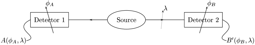
Figure 1: The experiment setup and some associated notation. The source emits a pair of spin-${}^{1}/_{2}$ particles in the singlet state, and $\lambda$ denotes the “hidden variable” to be used in the local hidden-variable model.

In ineq. (2) the notation is somewhat shortened, so that $A=A(\phi_{A},\lambda)$ and $B=B(\phi_{B},\lambda)$ pertains to the first detector while $B^{\prime}=B^{\prime}(\phi_{B},\lambda)$ and $C^{\prime}=C^{\prime}(\phi_{C},\lambda)$ pertains to the second, and the expressions $E(AB^{\prime})$, $E(AC^{\prime})$, and $E(BC^{\prime})$ are correlations of the results at detector 1 and detector 2 for different detector orientations. The results are labeled “spin up” ($\uparrow$ or $+1$) and “spin down” ($\downarrow$ or $-1$), and the key property of the singlet state in this context is the total anticorrelation of the measurement results when the detectors are equally oriented. In the notation in Fig. 1,

$$B^{\prime}(\phi_{B},\lambda)=-A(\phi_{A},\lambda)\;\text{ if }\;\phi_{B}=\phi_{A},$$ (3)

except on a set of zero probability.

If a local realistic (or “local hidden-variable”) model is possible, the inequality (2) holds, and the conclusion is that if the inequality is violated, no such model is possible. Since the derivation of the statistics of the singlet state is available in many standard textbooks on quantum mechanics, it will not be repeated here. The probabilities are (with $\theta=\phi_{B}-\phi_{A}$):

$$P_{++}^{\psi}=\frac{1-\cos(\theta)}{4}$$ (4a)

$$P_{+-}^{\psi}=\frac{1+\cos(\theta)}{4}$$ (4b)

$$P_{-+}^{\psi}=\frac{1+\cos(\theta)}{4}$$ (4c)

$$P_{--}^{\psi}=\frac{1-\cos(\theta)}{4},$$ (4d)

and the correlation obtained from this is

$$E^{\psi}(AB^{\prime})=P_{++}^{\psi}-P_{+-}^{\psi}-P_{-+}^{\psi}+P_{--}^{\psi}=-\cos(\theta).$$ (5)

Needless to say, the correlation obtained from quantum mechanics violates the Bell inequality, so there can be no local hidden-variable model (in the ideal case).

The original spin-${}^{1}/_{2}$ formulation will be retained in this paper, whereas present experiments in this context are most often performed with correlated photons which yield similar statistics for results labeled “horizontal polarization” ($\leftrightarrow$ or $+1$) and “vertical polarization” ($\updownarrow$ or $-1$). Quite a number of experiments of this kind have been performed (see e.g. Refs. [3, 4, 5, 6]), and although many experiments to date are reported to violate the Bell inequality, there are some problems, most notably detector inefficiency and lowered visibility (see e.g. Refs. [2, 7, 8, 9, 10]). The efficiency problem concerns the possibility of missing a detection altogether, while the visibility problem concerns the possibility of getting an erroneous detection, i.e., a detection that is converted from $+1$ to $-1$ or vice versa by an error. These two problems have a slightly different effect on the inequality.

Lowered efficiency does not change the correlation at all, provided the errors are independent and single events are discarded (events where both particles are missed are discarded automatically, so to speak). Therefore this would not seem to be a problem. Unfortunately, the inequality itself is influenced, as the original Bell inequality is simply not valid in an inefficient experiment. Letting $\eta$ be the efficiency of the detectors, and $E_{AB^{\prime}}(AB^{\prime})$ be the correlation where the single events (and no-detection events) have been removed, it is possible to derive the following generalized inequality [2]:

$$\bigl{|}E_{AB^{\prime}}(AB^{\prime})-E_{AC^{\prime}}(AC^{\prime})\bigr{|}\leq\frac{4}{\eta}-3+E_{BC^{\prime}}(BC^{\prime}),$$ (6)

In the form given here, the inequality is valid for constant efficiency and independent errors. As is evident from the above inequality, when $\eta$ decreases, the inequality becomes less restrictive on the correlations. The inequality is violated by the singlet state when $\eta>{}^{8}/_{9}\approx 88.89\%$, but using the Clauser-Horne-Shimony-Holt (CHSH) inequality [7] the bound is lower [2, 10]:

$$\bigl{|}E_{AC^{\prime}}(AC^{\prime})-E_{AD^{\prime}}(AD^{\prime})\bigr{|}+\bigl{|}E_{BC^{\prime}}(BC^{\prime})+E_{BD^{\prime}}(BD^{\prime})\bigr{|}\leq\frac{4}{\eta}-2.$$ (7)

Here, the bound is $\eta>2(\sqrt{2}-1)\approx 82.83\%$ (actually, this bound is necessary and sufficient [10]).

Lowered visibility is also a problem in the Bell inequality, because it needs full visibility to retain the total anticorrelation in (3). However, the CHSH inequality does not need (3) and is not changed by lowered visibility, so this inequality will be used below. The effect is instead that the amplitude of the correlation function is lowered, and using the parameter $v$ as a measure of the visibility,

$$E^{\text{nonideal}}_{AB^{\prime}}(AB^{\prime})=-v\cos(\theta),$$ (8)

which lowers the violation of the CHSH inequality. Since we have removed the single (and no-detection) events in the correlation, the efficiency $\eta$ does not appear in the above expression (but the effect of a lowered $\eta$ is included in the inequality (7)).

In the nonideal case, we have the following probabilities for constant detector efficiency and independent errors:

$$P(\text{detection of one particle})=\eta,$$ (9)

$$P(\text{detection of both particles})=\eta^{2}.$$ (10)

At either of the detectors, the single-particle probabilities are equal

$$P_{+}=P_{-}=\frac{\eta}{2},$$ (11)

and on measurement setup as a whole, the double-particle probabilities are

$$P^{\text{nonideal}}_{++}=\eta^{2}\frac{1-v\cos(\theta)}{4}$$ (12a)

$$P^{\text{nonideal}}_{+-}=\eta^{2}\frac{1+v\cos(\theta)}{4}$$ (12b)

$$P^{\text{nonideal}}_{-+}=\eta^{2}\frac{1+v\cos(\theta)}{4}$$ (12c)

$$P^{\text{nonideal}}_{--}=\eta^{2}\frac{1-v\cos(\theta)}{4}.$$ (12d)

In the construction below, the case of full visibility will be investigated as a starting point, leaving the case of lowered visibility to Section 3. In Section 4, the bounds in $\eta$ and $v$ for the model will be compared to the bounds in the Bell (or really, the CHSH) inequality. Finally, some concluding remarks will be made in Section 5.

2 Local variables: Detector inefficiency

The model is inspired by a simple type of model often seen in the literature, where the hidden variable $\lambda$ is simply an angular coordinate (e.g. [11, 12]), and the measurement results and the detection errors depend only on the orientation of the detector with respect to $\lambda$. In the below construction, an extension is made so that $\lambda$ is the pair $\lambda=(\phi,r)$ consisting of an angular variable $\phi\in[0,2\pi]$, which may be thought of as the “spin orientation”, along with another variable $r\in[0,1]$, the “detection parameter”. For each pair, the hidden variable $\lambda$ has a definite value, and the whole ensemble is taken to be an even distribution in the rectangle $(\phi,r)\in[0,2\pi]\times[0,1]$.

To visualize the model and to simplify the presentation, a series of figures will be used, where the “detector patterns” will show the experimental results for different values of $\lambda$. The sinusoidal form of the probabilities is the first aim to fulfill in the model, so initially the other desired properties will not be present in the model (see Figs. 2 and 3).

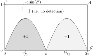
Figure 2: The detector pattern at detector 1. To get the sinusoidal form of the probabilities, the detector pattern should be sinusoidal at least at one detector.

The measurement results (and the detection errors) are given in the figures, and the procedure to obtain the measurement result is as follows: at detector 1, the value of $\phi$ is shifted to $\phi^{\prime}=\phi-\phi_{A}$ ($r$ is not changed), and the result is read off in Fig. 2.

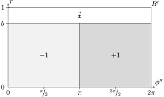
Figure 3: The pattern at detector 2.

At detector 2 the procedure is similar, but in this case the shift is $\phi^{\prime\prime}=\phi-\phi_{B}$. The result is $+1$ $(-1)$ when $\lambda$ falls in an area marked $+1$ $(-1)$, resp.. If $\lambda$ should happen to fall in an area marked $\nexists$, a measurement error (non-detection) occurs and the random variable $A$ ($B^{\prime}$) is not assigned a value (c.f. Ref. [2]).

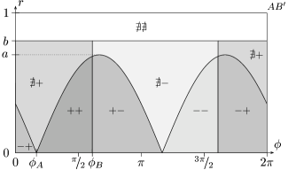
Figure 4: The detector patterns from Figs. 2 and 3 interposed in the $\lambda$-plane.

The probabilities for the coincident detections are now possible to calculate using Fig. 4, where the detector patterns have been interposed in the $\lambda$-plane with the proper shifts. E.g., the probability of getting $A=B^{\prime}=+1$ is the size of the area marked “$++$” (the size is the area divided by $2\pi$, because the total probability is one, whereas the total area is $2\pi$, also use $\theta=\phi_{B}-\phi_{A}$):

$$P_{++}=\frac{1}{2\pi}\int_{0}^{\theta}a\sin(\phi)d\phi=\frac{a(1-\cos(\theta))}{2\pi},$$ (13)

which has the sinusoidal form we want. Note that the calculation above is only valid if

$$0\leq a\leq b\leq 1,$$ (14)

and it is easy to see that the probability would not be sinusoidal if $a>b$. Thus, the model has the required form of the probabilities and constant efficiency, but an unwanted property is that the efficiencies of the detectors are different:

$$\eta_{B^{\prime}}=b,$$ (15)

while

$$\eta_{A}=\frac{2}{2\pi}\int_{0}^{\pi}a\sin(\phi)d\phi=\frac{2a}{\pi}\leq\frac{2b}{\pi}<b.$$ (16)

To resolve this, one way is to lower the efficiency of detector 2 by simply inserting random detection errors at that detector (which would yield the model described in [12]), but there is another way of resolving the problem, by symmetrizing the model (see Figs. 5 and 6).

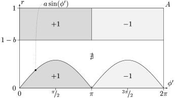
Figure 5: The detector pattern for detector 1 in the symmetrized model.

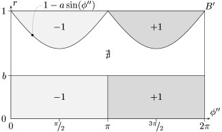
Figure 6: The detector pattern for detector 2 in the symmetrized model.

In this model, the parameters $a$ and $b$ are subject to the conditions

$$0\leq a\leq b\leq{}^{1}/_{2}.$$ (17)

The efficiency is obviously constant at

$$\eta=\eta_{A}=\eta_{B^{\prime}}=\frac{2a}{\pi}+b.$$ (18)

The errors should be independent, i.e.,

$$\eta^{2}=\frac{4a}{\pi},$$ (19)

and we have

$$\left\{\begin{split}a&=\frac{\pi\eta^{2}}{4}\\ b&=\eta-\frac{\eta^{2}}{2}.\end{split}\right.$$ (20)

Figure 7: Comparison of $a$ and $b$ (i.e., $a\leq b$).

By using (17) we arrive at the comparison of $a$ and $b$ in Fig. 7, and thus, the interval at which we may use this model is

$$0\leq\eta\leq\frac{4}{2+\pi}\approx 0.7780,$$ (21)

i.e., the model described above is usable up to $77.80\%$ efficiency. The probability of “++” in the symmetrized model is twice that in eqn. (13) by the symmetrization, which is

$$P_{++}=2\frac{a(1-\cos(\theta))}{2\pi}=\eta^{2}\frac{1-\cos(\theta)}{4},$$ (22)

as prescribed in (12a) using $v=1$, and the other probabilities are checked in the same manner.

3 Local variables: Visibility

Even though present experiments regularly have a high visibility (e.g. $97\%$ in Ref. [6]) it would be interesting to include this effect in the model presented in the previous section. The visibility is lowered in the model by adding random erroneous detections in it (see Fig. 8).

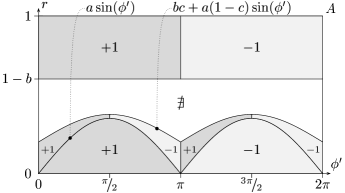
Figure 8: The detector pattern for detector 1 in the symmetrized model with lowered visibility. The detector pattern for detector 2 is symmetric in a similar fashion as in the previous section.

Also in this model, the parameters $a$ and $b$ are subject to the conditions

$$0\leq a\leq b\leq{}^{1}/_{2},$$ (23)

while the parameter $c$ is subject to the condition $0\leq c\leq 1$ and is the amount of errors added in the model, so that when $c=0$ we have full visibility. The sinusoidal pattern is not changed, in order not to change the general behavior of the probabilities. The efficiency is constant at

$$\eta=b+\bigl{(}bc+\frac{2a(1-c)}{\pi}\bigr{)}.$$ (24)

while the independence of the errors yields

$$\eta^{2}=2\bigl{(}bc+\frac{2a(1-c)}{\pi}\bigr{)}.$$ (25)

The visibility is the amount of “correct results” at equal detector orientations:

$$v=\frac{4a}{\pi}\Big{/}\eta^{2},$$ (26)

and after a simple calculation

$$\left\{\begin{split}a&=\frac{\pi v\eta^{2}}{4}\\ b&=\eta-\frac{\eta^{2}}{2}\\ c&=\frac{\eta(1-v)}{2-\eta(1+v)}.\end{split}\right.$$ (27)

The probability of the result “++” is obtained by the following expression, where the limits of the first integral is obtained by the symmetry of the model

$$\begin{split}P_{++}&=\frac{2}{2\pi}\int_{0}^{\frac{\pi}{2}}\bigl{(}bc+a(1-c)\sin(\phi)\bigr{)}-a\sin(\phi)d\phi\\ &\qquad+\frac{2}{2\pi}\int_{0}^{\theta}a\sin(\phi)d\phi\\ &=\frac{1}{2}\Bigl{(}bc+\frac{2a(1-c)}{\pi}\Bigr{)}-\frac{a}{\pi}\cos(\theta)\\ &=\frac{\eta^{2}}{4}-\frac{v\eta^{2}}{4}\cos(\theta),\end{split}$$ (28)

exactly as in (12a).

Figure 9: Comparison of $a$ and $b$ in the model including visibility (i.e., $a\leq b$).

Examining the parameters, $b$ is as before and the change in $a$ is an extra factor $v$, and comparing $a$ and $b$ (see Fig. 9) we can see that if $\eta$ is less than the $77.80\%$ discussed in the previous section, there is no restriction on the visibility. If $\eta$ is larger than this bound, the interval at which we may use this model is (use (27) in (23))

$$v\leq\frac{1}{\pi}\bigl{(}\frac{4}{\eta}-2\bigr{)}.$$ (29)

This excludes the point $\eta=1$, $v=1$, where $c$ is on the form ${}^{0}/_{0}$, and for all other values of $\eta$ and $v$, $0\leq c\leq 1$. One may especially note that if $\eta=1$, the interval is

$$v\leq\frac{2}{\pi}.$$ (30)

4 The role of the Bell inequality

In the Bell inequality (or really the CHSH inequality), the $82.83\%$ is obtained by choosing detector orientations so that the violation of the inequality is maximized:

$$\phi_{A}=0,\;\phi_{B}={}^{\pi}/_{2},\;\phi_{C}={}^{\pi}/_{4},\text{ and }\phi_{D}={}^{3\pi}/_{4}.$$ (31)

With these choices of angles in the CHSH inequality, and using $E^{\text{nonideal}}_{AB^{\prime}}$ from (8), we obtain $2\sqrt{2}v\leq 4\eta^{-1}-2,$ or

$$v\leq\frac{1}{2\sqrt{2}}\bigl{(}\frac{4}{\eta}-2\bigr{)},$$ (32)

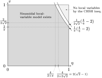
Figure 10: The region where the model is usable as compared to the region where no local hidden-variable model is possible.

In Fig. 10, there is a region where the local-variable model does not work which is not ruled out by the CHSH inequality. A reason for this may be that the correlation is not tested as a function in the CHSH inequality, but only the values at certain points are used (see Fig. 11).

Figure 11: The points where the correlation is tested in the CHSH inequality. Note the small difference between the sinusoidal curve and the dashed curve consisting of line segments.

It would be interesting to know if the straight-line correlation (the dashed line in Fig. 11) is possible to model in the empty region in Fig. 10. To construct a model for this case, one uses the procedure outlined in the previous sections, where the derivative of the correlation is used to determine the general outline of the pattern. The correlation is composed of straight lines, so therefore the pattern should be staircased (i.e., constant derivative). The derivative should be low from $0$ to ${}^{\pi}/_{4}$, then somewhat higher from ${}^{\pi}/_{4}$ to ${}^{3\pi}/_{4}$, and then again low from ${}^{3\pi}/_{4}$ to $\pi$. The relation between the derivatives is

$$\frac{1-\frac{1}{\sqrt{2}}}{\frac{\pi}{4}}\Bigg{/}\frac{\frac{1}{\sqrt{2}}}{\frac{\pi}{4}}=\sqrt{2}-1.$$ (33)

The procedure continues, and eventually yields (after addition of random errors to lower the visibility) the construction in Fig. 12.

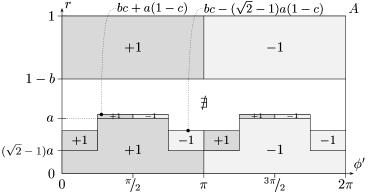
Figure 12: The detector pattern for detector 1 in the straight-line model with lowered visibility. The detector pattern for detector 2 is chosen symmetrically.

Here, our equations are

$$\eta=b+\bigl{(}bc+\frac{a(1-c)}{\sqrt{2}}\bigr{)},$$ (34)

$$\eta^{2}=2\bigl{(}bc+\frac{a(1-c)}{\sqrt{2}}\bigr{)},$$ (35)

and

$$v=\sqrt{2}a\Big{/}\eta^{2},$$ (36)

and we arrive at

$$\left\{\begin{split}a&=\frac{v\eta^{2}}{\sqrt{2}}\;\;\Bigl{(}=\frac{2\sqrt{2}v\eta^{2}}{4}\Bigr{)}\\ b&=\eta-\frac{\eta^{2}}{2}\\ c&=\frac{\eta(1-v)}{2-\eta(1+v)}.\end{split}\right.$$ (37)

Note that the only change from eqn. (27) is that the constant $\pi$ in the expression for $a$ is changed to $2\sqrt{2}$. This yields the allowed range as

$$v\leq\frac{1}{2\sqrt{2}}\bigl{(}\frac{4}{\eta}-2\bigr{)}.$$ (38)

And this is exactly the bound from the CHSH inequality.

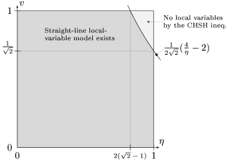
Figure 13: The region where the straight-line model is usable, as compared to the region where no local hidden-variable model is possible.

In essence, we have an explicit model proving the necessity of having $\eta>82.83\%$ to contradict local realism in the CHSH inequality. The bound was shown to be necessary and sufficient already in Ref. [10], but here an explicit counter-example is obtained below the bound. In addition, the effect of lowered visibility is included in this construction.

The same construction for the straight-line case allows a higher visibility at a given efficiency than for the sinusoidal case. It seems natural that the sinusoidal form of the correlation is somewhat more difficult to model than the straight-line form. This enables us to conjecture that the bound would be lowered if a result that utilizes the full sinusoidal form of the correlation would be used instead of the CHSH inequality.

5 Conclusions

We have a local-variable model yielding the sinusoidal probabilities obtained from quantum mechanics, valid for visibilities in the range

$$v\leq\frac{1}{\pi}\big{(}\frac{4}{\eta}-2\big{)}.$$ (29)

Experimental results to date may be described using this model by using the proper values of efficiency and visibility obtained in the experiment. Although the visibility is high in present experiments, the efficiency is still too low to yield a decisive test whether Nature violates local realism or not (if preferred, whether Nature violates the Bell inequality or not), e.g., in [6] the visibility $v\approx 97\%$ and the efficiency $\eta\approx 5\%$.

The model is well-behaved in that the efficiency does not vary and the errors are independent, and neither the non-detection errors nor the wrong-result errors depend on the detector orientation. Thus, there is no test on the properties of the errors that would invalidate local variables for the singlet state below the bound (29).

In all, we have a model which has:

QM statistics

Local variables

Independent errors

$78.80\%$ efficiency

$100\%$ visibility

or, if preferred:

QM statistics

Local variables

Independent errors

$63.66\%$ visibility

$100\%$ efficiency

and there is currently no experiment result that invalidates this model.

The question remains if there is a possibility to devise a model where the bound (29) is on the level of the CHSH inequality, while keeping the sinusoidal form of the correlation. By the result in the previous section, it is more probable that a result utilizing the whole sinusoidal form of the correlation function rather than the values at a few points, would lower the bound to (29). The efficiency bound would then be lowered to $\eta>78.80\%$ for a violation of local realism.

References

- [1] J. S. Bell. On the Einstein-Podolsky-Rosen paradox. Physics, 1:195–200, 1964.
- [2] Jan-Åke Larsson. The Bell inequality and detector inefficiency. Phys. Rev. A, 57:3304–3308, 1998.
- [3] Alain Aspect, Philippe Grangier, and Gérard Roger. Experimental tests of realistic local theories via Bell’s theorem. Phys. Rev. Lett., 47:460–463, 1981.
- [4] Alain Aspect, Philippe Grangier, and Gérard Roger. Experimental realization of Einstein-Podolsky-Rosen-Bohm Gedankenexperiment: A new violation of Bell’s inequalities. Phys. Rev. Lett., 49:91–94, 1982.
- [5] Alain Aspect, Jean Dalibard, and Gérard Roger. Experimental test of Bell’s inequalities using time-varying analyzers. Phys. Rev. Lett., 49:1804–1807, 1982.
- [6] Gregor Weihs, Thomas Jennewein, Christoph Simon, Harald Weinfurter, and Anton Zeilinger. Violation of Bell’s inequality under strict Einstein locality conditions. Phys. Rev. Lett., 81:5039–5043, 1998.
- [7] John F. Clauser, Michael A. Horne, Abner Shimony, and Richard A. Holt. Proposed experiment to test local hidden-variable theories. Phys. Rev. Lett., 23:880–884, 1969.
- [8] John F. Clauser and Michael A. Horne. Experimental consequences of objective local theories. Phys. Rev. D, 10:526–535, 1974.
- [9] John F. Clauser and Abner Shimony. Bell’s theorem: experimental tests and implications. Rep. Prog. Phys., 41:1881–1927, 1978.
- [10] Anupam Garg and N. D. Mermin. Detector inefficiencies in the Einstein-Podolsky-Rosen experiment. Phys. Rev. D, 35:3831–3835, 1987.
- [11] Jim Baggott. The meaning of quantum theory. Oxford Univ. Press, Oxford, 1992.
- [12] Emilio Santos. Unreliability of performed tests of Bell’s inequality using parametric down-converted photons. Phys. Lett. A, 212:10–14, 1996.