Excess noise for coherent radiation propagating through amplifying random media

Abstract

A general theory is presented for the photodetection statistics of coherent radiation that has been amplified by a disordered medium. The beating of the coherent radiation with the spontaneous emission increases the noise above the shot-noise level. The excess noise is expressed in terms of the transmission and reflection matrices of the medium, and evaluated using the methods of random-matrix theory. Inter-mode scattering between $N$ propagating modes increases the noise figure by up to a factor of $N$, as one approaches the laser threshold. Results are contrasted with those for an absorbing medium.

]

I Introduction

The coherent radiation emitted by a laser has a noise spectral density $P$ equal to the time-averaged photocurrent $\bar{I}$. This noise is called photon shot noise, by analogy with electronic shot noise in vacuum tubes. If the radiation is passed through an amplifying medium, $P$ increases more than $\bar{I}$ because of the excess noise due to spontaneous emission [1]. For an ideal linear amplifier, the (squared) signal-to-noise ratio $\bar{I}^{2}/P$ drops by a factor of two as one increases the gain. One says that the amplifier has a noise figure of $2$. This is a lower bound on the excess noise for a linear amplifier [2].

Most calculations of the excess noise assume that the amplification occurs in a single propagating mode. (Recent examples include work by Loudon and his group [3, 4].) The minimal noise figure of $2$ refers to this case. Generalisation to amplification in a multi-mode waveguide is straightforward if there is no scattering between the modes. The recent interest in amplifying random media [5] calls for an extension of the theory of excess noise to include inter-mode scattering. Here we present such an extension.

Our central result is an expression for the probability distribution of the photocount in terms of the transmission and reflection matrices $t$ and $r$ of the multi-mode waveguide. (The noise power $P$ is determined by the variance of this distribution.) Single-mode results in the literature are recovered for scalar $t$ and $r$. In the absence of any incident radiation our expression reduces to the known photocount distribution for amplified spontaneous emission [6]. We find that inter-mode scattering strongly increases the excess noise, resulting in a noise figure that is much larger than $2$.

We present explicit calculations for two types of geometries, waveguide and cavity, distinguishing between photodetection in transmission and in reflection. We also discuss the parallel with absorbing media. We use the method of random-matrix theory [7] to obtain the required information on the statistical properties of the transmission and reflection matrices of an ensemble of random media. Simple analytical results follow if the number of modes $N$ is large (i.e. for high-dimensional matrices). Close to the laser threshold, the noise figure ${\cal F}$ exhibits large sample-to-sample fluctuations, such that the ensemble average diverges. We compute for arbitrary $N\geq 2$ the distribution $p({\cal F})$ of ${\cal F}$ in the ensemble of disordered cavities, and show that ${\cal F}=N$ is the most probable value. This is the generalisation to multi-mode random media of the single-mode result ${\cal F}=2$ in the literature.

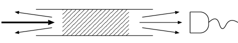
FIG. 1.: Coherent light (thick arrow) is incident on an amplifying medium (shaded), embedded in a waveguide. The transmitted radiation is measured by a photodetector.

II Formulation of the problem

We consider an amplifying disordered medium embedded in a waveguide that supports $N(\omega)$ propagating modes at frequency $\omega$ (see Fig. 1). The amplification could be due to stimulated emission by an inverted atomic population or to stimulated Raman scattering [1]. A negative temperature $T<0$ describes the degree of population inversion in the first case or the density of the material excitation in the second case [3]. A complete population inversion or vanishing density corresponds to the limit $T\to 0$ from below. The minimal noise figure mentioned in the introduction is reached in this limit. The amplification rate $1/\tau_{a}$ is obtained from the (negative) imaginary part $\epsilon^{\prime\prime}$ of the (relative) dielectric constant, $1/\tau_{a}=\omega|\epsilon^{\prime\prime}|$. Disorder causes multiple scattering with rate $1/\tau_{s}$ and (transport) mean free path $l=c\tau_{s}$ (with $c$ the velocity of light in the medium). We assume that $\tau_{s}$ and $\tau_{a}$ are both $\gg 1/\omega$, so that scattering as well as amplification occur on length scales large compared to the wavelength. The waveguide is illuminated from one end by monochromatic radiation (frequency $\omega_{0}$, mean photocurrent $I_{0}$) in a coherent state. For simplicity, we assume that the illumination is in a single propagating mode (labelled ${m_{0}}$). At the other end of the waveguide, a photodetector detects the outcoming radiation. We assume, again for simplicity, that all $N$ outgoing modes are detected with equal efficiency $\alpha$.

We denote by $p(n)$ the probability to count $n$ photons within a time $\tau$. Its first two moments determine the mean photocurrent $\bar{I}$ and the noise power $P$, according to

$$\bar{I}=\frac{1}{\tau}\overline{n},\qquad P=\lim_{\tau\to\infty}\frac{1}{\tau}\left(\overline{n^{2}}-\overline{n}^{2}\right)\;.$$ (1)

(The definition of $P$ is equivalent to $P=\int_{-\infty}^{\infty}dt\,\overline{\delta I(0)\delta I(t)}$, with $\delta I=I-\bar{I}$ the fluctuating part of the photocurrent.) It is convenient to compute the generating function $F(\xi)$ for the factorial cumulants $\kappa_{j}$, defined by

$$F(\xi)=\sum_{j=1}^{\infty}\frac{\kappa_{j}\xi^{j}}{j!}=\ln\left(\sum_{n=0}^{\infty}(1+\xi)^{n}p(n)\right)\;.$$ (2)

One has $\overline{n}=\kappa_{1},\overline{n^{2}}=\kappa_{2}+\kappa_{1}(1+\kappa_{1})$.

The outgoing radiation in mode $n$ is described by an annihilation operator $a_{n}^{{\text{out}}}(\omega)$, using the convention that modes $1,2,\ldots,N$ are on the left-hand-side of the medium and modes $N+1,\ldots,2N$ are on the right-hand-side. The vector $a^{{\text{out}}}$ consists of the operators $a_{1}^{{\text{out}}},a_{2}^{{\text{out}}},\ldots,a_{2N}^{{\text{out}}}$. Similarly, we define a vector $a^{{\text{in}}}$ for incoming radiation. These two sets of operators each satisfy the bosonic commutation relations

$$[a_{n}(\omega),a_{m}^{\dagger}(\omega^{\prime})] = \delta_{nm}\delta(\omega-\omega^{\prime})\;,$$ (4)

$${[}a_{n}(\omega),a_{m}(\omega^{\prime})] = 0\;,$$ (5)

and are related by the input-output relations [3, 8, 9]

$$a^{{\text{out}}}(\omega)=S(\omega)a^{{\text{in}}}(\omega)+V(\omega)c^{\dagger}(\omega)\;.$$ (6)

We have introduced the $2N\times 2N$ scattering matrix $S$, the $2N\times 2N$ matrix $V$, and the vector $c$ of $2N$ bosonic operators. The scattering matrix $S$ can be decomposed into four $N\times N$ reflection and transmission matrices,

$$S=\left(\begin{array}[]{cc}r^{\prime}&t^{\prime}\\ t&r\end{array}\right)\;.$$ (7)

Reciprocity imposes the conditions $t^{\prime}=t^{T}$, $r=r^{T}$, and $r^{\prime}=r^{\prime T}$.

The operators $c$ account for spontaneous emission in the amplifying medium. They satisfy the bosonic commutations relation (II), which implies that

$$VV^{\dagger}=SS^{\dagger}-{\openone}\;.$$ (8)

Their expectation values are

$$\langle c_{n}(\omega)c_{m}^{\dagger}(\omega^{\prime})\rangle=-\delta_{nm}\delta(\omega-\omega^{\prime})f(\omega,T)\;,$$ (9)

with the Bose-Einstein function

$$f(\omega,T)=\left[\exp(\hbar\omega/kT)-1\right]^{-1}$$ (10)

evaluated at negative temperature $T$ ($<0$).

III Calculation of the generating function

The probability $p(n)$ that $n$ photons are counted in a time $\tau$ is given by [10, 11]

$$p(n)=\frac{1}{n!}\langle:W^{n}e^{-W}:\rangle\;,$$ (11)

where the colons denote normal ordering with respect to $a^{{\text{out}}}$, and

$$W=\alpha\int_{0}^{\tau}dt\sum_{n=N+1}^{2N}a_{n}^{{\text{out}}\dagger}(t)a_{n}^{{\text{out}}}(t)\;,$$ (12)

$$a^{{\text{out}}}_{n}(t)=(2\pi)^{-1/2}\int_{0}^{\infty}\text{d}\omega\,e^{-i\omega t}a^{\text{out}}_{n}(\omega)\;.$$ (13)

The generating function (2) becomes

$$F(\xi)=\ln\langle:e^{\xi W}:\rangle\;.$$ (14)

Expectation values of a normally ordered expression are readily computed using the optical equivalence theorem [12]. Application of this theorem to our problem consists in discretising the frequency in infinitesimally small steps of $\Delta$ (so that $\omega_{p}=p\Delta$) and then replacing the annihilation operators $a^{\text{in}}_{n}(\omega_{p}),c_{n}(\omega_{p})$ by complex numbers $a^{\text{in}}_{np}$, $c_{np}$ (or their complex conjugates for the corresponding creation operators). The coherent state of the incident radiation corresponds to a non-fluctuating value of $a_{np}^{\text{in}}$ with $|a_{np}^{\text{in}}|^{2}=\delta_{n{m_{0}}}\delta_{pp_{0}}2\pi I_{0}/\Delta$ (with $\omega_{0}=p_{0}\Delta$). The thermal state of the spontaneous emission corresponds to uncorrelated Gaussian distributions of the real and imaginary parts of the numbers $c_{np}$, with zero mean and variance $\langle(\text{Re}\,c_{np})^{2}\rangle=\langle(\text{Im}\,c_{np})^{2}\rangle=-\frac{1}{2}f(\omega_{p},T)$. (Note that $f<0$ for $T<0$.) To evaluate the characteristic function (14) we need to perform Gaussian averages. The calculation is described in the appendix.

The result takes a simple form in the long-time regime $\omega_{c}\tau\gg 1$, where $\omega_{c}$ is the frequency within which $S(\omega)$ does not vary appreciably. We find

$$F(\xi)=F_{\text{exc}}(\xi)$$ (15)

$$\quad\mbox{}-\frac{\tau}{2\pi}\int_{0}^{\infty}\ln\|{\openone}-\alpha\xi f({\openone}-rr^{\dagger}-tt^{\dagger})\|\,d\omega\;,$$ (16)

$$F_{\text{exc}}(\xi)=\alpha\xi\tau I_{0}$$ (17)

$$\quad{}\times\left(t^{\dagger}\left[{\openone}-\alpha\xi f({\openone}-rr^{\dagger}-tt^{\dagger})\right]^{-1}t\right)_{{m_{0}}{m_{0}}}\;,$$ (18)

where $\|\cdots\|$ denotes the determinant and $(\cdots)_{{m_{0}}{m_{0}}}$ the ${m_{0}}{,}{m_{0}}$-element of a matrix. In Eq. (18) the functions $f$, $t$, and $r$ are to be evaluated at $\omega=\omega_{0}$. The integral in Eq. (16) is the generating function for the photocount due to amplified spontaneous emission obtained in Ref. [6]. It is independent of the incident radiation and can be eliminated in a measurement by filtering the output through a narrow frequency window around $\omega_{0}$. The function $F_{\text{exc}}(\xi)$ describes the excess noise due to the beating of the coherent radiation with the spontaneous emission. The expression (18) is the central result of this paper.

By expanding $F(\xi)$ in powers of $\xi$ we obtain the factorial cumulants, in view of Eq. (2). We will in what follows consider only the contribution from $F_{\text{exc}}(\xi)$, assuming that the contribution from the integral over $\omega$ has been filtered out as mentioned above. We find

$$\kappa_{k}=k!\alpha^{k}\tau f^{k-1}I_{0}[t^{\dagger}\left({\openone}-rr^{\dagger}-tt^{\dagger}\right)^{k-1}t]_{{m_{0}}{m_{0}}}\;,$$ (19)

where again $\omega=\omega_{0}$ is implied. The mean photocurrent $\bar{I}=\kappa_{1}/\tau$ and the noise power $P=(\kappa_{2}+\kappa_{1})/\tau$ become

$$\bar{I}=\alpha I_{0}\left(t^{\dagger}t\right)_{{m_{0}}{m_{0}}}\;,\quad P=\bar{I}+P_{\text{exc}}\;,$$ (20)

$$P_{\text{exc}}=2\alpha^{2}fI_{0}[t^{\dagger}\left({\openone}-rr^{\dagger}-tt^{\dagger}\right)t]_{{m_{0}}{m_{0}}}\;.$$ (21)

The noise power $P$ exceeds the shot noise $\bar{I}$ by the amount $P_{\text{exc}}$.

The formulas above are easily adapted to a measurement in reflection by making the exchange $r\rightarrow t^{\prime}$, $t\rightarrow r^{\prime}$. For example, the mean reflected photocurrent is $\bar{I}=\alpha I_{0}\left(r^{\prime\dagger}r^{\prime}\right)_{{m_{0}}{m_{0}}}$, while the excess noise is

$$P_{\text{exc}}=2\alpha^{2}fI_{0}[r^{\prime\dagger}\left({\openone}-r^{\prime}r^{\prime\dagger}-t^{\prime}t^{\prime\dagger}\right)r^{\prime}]_{{m_{0}}{m_{0}}}\;.$$ (22)

IV Noise figure

The noise figure ${\cal F}$ is defined as the (squared) signal-to-noise ratio at the input $I_{0}^{2}/P_{0}$, divided by the signal-to-noise ratio at the output, $\bar{I}^{2}/P$. Since $P_{0}=I_{0}$ for coherent radiation at the input, one has ${\cal F}=(P_{\text{exc}}+\bar{I})I_{0}/\bar{I}^{2}$, hence

$${\cal F}=-2f\frac{\left(t^{\dagger}rr^{\dagger}t+t^{\dagger}tt^{\dagger}t\right)_{{m_{0}}{m_{0}}}}{\left(t^{\dagger}t\right)_{{m_{0}}{m_{0}}}^{2}}+\frac{1+2\alpha f}{\alpha\left(t^{\dagger}t\right)_{{m_{0}}{m_{0}}}}\;.$$ (23)

The noise figure is independent of $I_{0}$. For large amplification the second term on the right-hand-side can be neglected relative to the first, and the noise figure becomes also independent of the detection efficiency $\alpha$. The minimal noise figure for given $r$ and $t$ is reached for an ideal detector ($\alpha=1$) and at complete population inversion ($f=-1$).

Since $(t^{\dagger}rr^{\dagger}t+t^{\dagger}tt^{\dagger}t)_{{m_{0}}{m_{0}}}=\sum_{k}|(t^{\dagger}r)_{{m_{0}}k}|^{2}+\sum_{k}|(t^{\dagger}t)_{{m_{0}}k}|^{2}\geq(t^{\dagger}t)_{{m_{0}}{m_{0}}}^{2}$, one has ${\cal F}\geq-2f$ for large amplification (when the second term on the right-hand-side of Eq. (23) can be neglected). The minimal noise figure ${\cal F}=2$ at complete population inversion is reached in the absence of reflection [$(t^{\dagger}r)_{{m_{0}}k}=0$] and in the absence of inter-mode scattering [$(t^{\dagger}t)_{{m_{0}}k}=0$ if $k\neq{m_{0}}$]. This is realised in the single-mode theories of Refs. [3, 4]. Our result (23) generalises these theories to include scattering between the modes, as is relevant for a random medium.

These formulas apply to detection in transmission. For detection in reflection one has instead

$${\cal F}=-2f\frac{\left(r^{\prime\dagger}t^{\prime}t^{\prime\dagger}r^{\prime}+r^{\prime\dagger}r^{\prime}r^{\prime\dagger}r^{\prime}\right)_{{m_{0}}{m_{0}}}}{\left(r^{\prime\dagger}r^{\prime}\right)_{{m_{0}}{m_{0}}}^{2}}+\frac{1+2\alpha f}{\alpha\left(r^{\prime\dagger}r^{\prime}\right)_{{m_{0}}{m_{0}}}}\;.$$ (24)

Again, for large amplification the second term on the right-hand-side may be neglected relative to the first. The noise figure then becomes smallest in the absence of transmission, when ${\cal F}=-2f(r^{\prime\dagger}r^{\prime}r^{\prime\dagger}r^{\prime})_{{m_{0}}{m_{0}}}(r^{\prime\dagger}r^{\prime})_{{m_{0}}{m_{0}}}^{-2}\geq-2f$. The minimal noise figure of $2$ at complete population inversion requires $(r^{\prime\dagger}r^{\prime}r^{\prime\dagger}r^{\prime})_{{m_{0}}{m_{0}}}=(r^{\prime\dagger}r^{\prime})_{{m_{0}}{m_{0}}}^{2}$, which is possible only in the absence of inter-mode scattering.

To make analytical progress in the evaluation of ${\cal F}$, we will consider an ensemble of random media, with different realisations of the disorder. For large $N$ and away from the laser threshold, the sample-to-sample fluctuations in numerators and denominators of Eqs. (23) and (24) are small, so we may average them separately. Furthermore, the “equivalent channel approximation” is accurate for random media [13], which says that the ensemble averages are independent of the mode index ${m_{0}}$. Summing over ${m_{0}}$, we may therefore write ${\cal F}$ as the ratio of traces, so the noise figure for a measurement in transmission becomes

$${\cal F}=-2fN\frac{\prec\text{tr}\,(t^{\dagger}rr^{\dagger}t+t^{\dagger}tt^{\dagger}t)\succ}{\prec\text{tr}\,t^{\dagger}t\succ^{2}}+N\frac{1+2\alpha f}{\alpha\prec\text{tr}\,t^{\dagger}t\succ}\;,$$ (25)

and similarly for a measurement in reflection. The brackets $\prec\cdots\succ$ denote the ensemble average.

V Applications

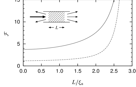
FIG. 2.: Noise figure of an amplifying disordered waveguide (length $L$, amplification length $\xi_{a}$) measured in transmission (solid line) and in reflection (dashed line). The curves are computed from Eqs. (26)–(31) for $\alpha=1$, $f=-1$, and $L/l=10$. The laser threshold is at $L/\xi_{a}=\pi$.

A Amplifying disordered waveguide

As a first example, we consider a weakly amplifying, strongly disordered waveguide of length $L$ (see inset of Fig. 2). Averages of the moments of $rr^{\dagger}$ and $tt^{\dagger}$ for this system have been computed by Brouwer [14] as a function of the number of propagating modes $N$, the mean free path $l$, and the amplification length $\xi_{a}=\sqrt{D\tau_{a}}$, where $1/\tau_{a}$ is the amplification rate and $D=cl/3$ is the diffusion constant. It is assumed that $1/N\ll l/\xi_{a}\ll 1$ but the ratio $L/\xi_{a}\equiv s$ is arbitrary. In this regime, sample-to-sample fluctuations are small, so the ensemble average is representative of a single system.

The results for a measurement in transmission are

$$\bar{I} = \frac{4\alpha l}{3L}I_{0}\frac{s}{\sin s}\;,$$ (26)

$$P_{\text{exc}} = \frac{2\alpha^{2}l}{3L}fI_{0}s\left[\frac{3}{\sin s}-\frac{2s-\,\text{cotan}\,s}{\sin^{2}s}\right.$$ (28)

$$\mbox{}\left.\quad\mbox{}+\frac{s\,\text{cotan}\,s-1}{\sin^{3}s}-\frac{s}{\sin^{4}s}\right]\;.$$

For a measurement in reflection, one finds

$$\bar{I} = \alpha I_{0}\left[1-\frac{4l}{3L}s\,\text{cotan}\,s\right]\;,$$ (29)

$$P_{\text{exc}} = \frac{2\alpha^{2}l}{3L}fI_{0}s\left[2\,\text{cotan}\,s-\frac{1}{\sin s}+\frac{\,\text{cotan}\,s}{\sin^{2}s}\right.$$ (31)

$${}\left.\quad\mbox{}+\frac{s\,\text{cotan}\,s-1}{\sin^{3}s}-\frac{s}{\sin^{4}s}\right]\;.$$

The noise figure ${\cal F}$ follows from ${\cal F}=(P_{\text{exc}}+\bar{I})I_{0}/\bar{I}^{2}$. It is plotted in Fig. 2. One notices a strong increase in ${\cal F}$ on approaching the laser threshold at $s=\pi$.

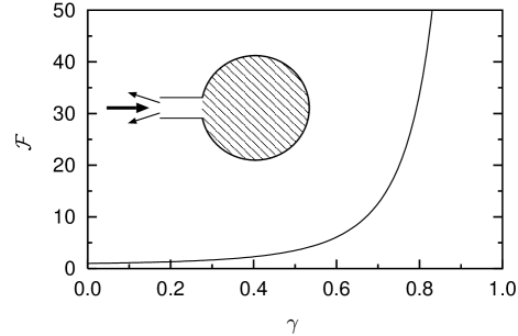
FIG. 3.: Noise figure of an amplifying disordered cavity, connected to a photodetector via an $N$-mode waveguide. The curve is the result (36), as a function of the dimensionless amplification rate $\gamma$. (Ideal detection efficiency, $\alpha=1$, and full population inversion, $f=-1$, are assumed in this plot.) The laser threshold occurs at $\gamma=1$.

B Amplifying disordered cavity

Our second example is an optical cavity filled with an amplifying random medium (see inset of Fig. 3). The radiation leaves the cavity through a waveguide supporting $N$ modes. The formulas for a measurement in reflection apply with $t=0$ because there is no transmission. The distribution of the eigenvalues of $r^{\dagger}r$ is known in the large-$N$ limit [15] as a function of the dimensionless amplification rate $\gamma=2\pi/N\tau_{a}\Delta\omega$ (with $\Delta\omega$ the spacing of the cavity modes near frequency $\omega_{0}$). The first two moments of this distribution are

$$N^{-1}\prec\text{tr}\,r^{\dagger}r\succ = \frac{1}{1-\gamma},$$ (32)

$$N^{-1}\prec\text{tr}\,r^{\dagger}rr^{\dagger}r\succ = \frac{2\gamma^{2}-2\gamma+1}{(1-\gamma)^{4}}\;.$$ (33)

The resulting photocurrent has mean and variance

$$\bar{I} = \alpha I_{0}\frac{1}{1-\gamma}\;,$$ (34)

$$P_{\text{exc}} = 2\alpha^{2}fI_{0}\gamma\frac{\gamma-\gamma^{2}-1}{(1-\gamma)^{4}}\;.$$ (35)

The resulting noise figure for $\alpha=1$ and $f=-1$,

$${\cal F}=\frac{1-\gamma+\gamma^{2}+\gamma^{3}}{\left(1-\gamma\right)^{2}}\;,$$ (36)

is plotted in Fig. 3. Again, we see a strong increase of ${\cal F}$ on approaching the laser threshold at $\gamma=1$.

VI Near the laser threshold

In the previous section we have taken the large-$N$ limit. In that limit the noise figure diverges on approaching the laser threshold. In this section we consider the vicinity of the laser threshold for arbitrary $N$.

The scattering matrix $S(\omega)$ has poles in the lower half of the complex plane. With increasing amplification, the poles shift upwards. The laser threshold is reached when a pole reaches the real axis, say at resonance frequency $\omega_{\text{th}}$. For $\omega$ near $\omega_{\text{th}}$ the scattering matrix has the generic form

$$S_{nm}=\frac{\sigma_{n}\sigma_{m}}{\omega-\omega_{\text{th}}+\frac{1}{2}i\Gamma-i/2\tau_{a}}\;,$$ (37)

where $\sigma_{n}$ is the complex coupling constant of the resonance to the $n$-th mode in the waveguide, $\Gamma$ is the decay rate, and $1/\tau_{a}$ the amplification rate. The laser threshold is at $\Gamma\tau_{a}=1$.

We assume that the incident radiation has frequency $\omega_{0}=\omega_{\text{th}}$. Substitution of Eq. (37) into Eq. (23) or (24) gives the simple result

$${\cal F}=\frac{-2f\Sigma}{|\sigma_{{m_{0}}}|^{2}},\;\Sigma=\sum_{n=1}^{2N}|\sigma_{n}|^{2}\;,$$ (38)

for the limiting value of the noise figure on approaching the laser threshold. The limit is the same for detection in transmission and in reflection. Since the coupling contant $|\sigma_{{m_{0}}}|^{2}$ to the mode ${m_{0}}$ of the incident radiation can be much smaller than the total coupling constant $\Sigma$, the noise figure (38) has large fluctuations. We need to consider the statistical distribution $p({\cal F})$ in the ensemble of random media. The typical (or modal) value of ${\cal F}$ is the value ${\cal F}_{\text{typ}}$ at which $p({\cal F})$ is maximal. We will see that this remains finite although the ensemble average $\prec{\cal F}\succ$ of ${\cal F}$ diverges.

A Waveguide geometry

We first consider the case of an amplifying disordered waveguide. The total coupling constant $\Sigma=\Sigma_{l}+\Sigma_{r}$ is the sum of the coupling constant $\Sigma_{l}=\sum_{n=1}^{N}|\sigma_{n}|^{2}$ to the left end of the waveguide and the coupling constant $\Sigma_{r}=\sum_{n=N+1}^{2N}|\sigma_{n}|^{2}$ to the right. The assumption of equivalent channels implies that

$$\prec 1/{\cal F}\succ=-\frac{1}{2fN}\prec\Sigma_{l}/\Sigma\succ=-\frac{1}{4fN}\;.$$ (39)

Since the average of $1/{\cal F}$ is finite, it is reasonable to assume that ${\cal F}_{\text{typ}}\approx\prec 1/{\cal F}\succ^{-1}=-4fN$, or ${\cal F}_{\text{typ}}\approx 4N$ for complete population inversion. The scaling with $N$ explains why the large-$N$ theory of the previous section found a divergent noise figure at the laser threshold. We conclude that the divergency of ${\cal F}$ at $L/\xi_{a}=\pi$ in Fig. 2 is cut off at a value of order $N$, if ${\cal F}$ is identified with the typical value ${\cal F}_{\text{typ}}$.

B Cavity geometry

In the case of an amplifying disordered cavity, we can make a more precise statement on $p({\cal F})$. Since there is only reflection there is only one $\Sigma=\sum_{n=1}^{N}|\sigma_{n}|^{2}$. The assumption of equivalent channels now gives

$$\prec 1/{\cal F}\succ=-\frac{1}{2fN}\;.$$ (40)

Following the same reasoning as in the case of the waveguide, we would conclude that ${\cal F}_{\text{typ}}\approx\prec 1/{\cal F}\succ^{-1}=-2fN$. We will see that this is correct within a factor of two.

To compute $p({\cal F})$ we need the distribution of the dimensionless coupling constants $u_{n}=\sigma_{n}/\sqrt{\Sigma}$. The $N$ complex numbers $u_{n}$ form a vector $\vec{u}$ of length $1$. According to random-matrix theory [7], the distribution $p(S)$ of the scattering matrix is invariant under unitary transformations $S\to USU^{T}$ (with $U$ an $N\times N$ unitary matrix). It follows that the distribution $p(\vec{u})$ of the vector $\vec{u}$ is invariant under rotations $\vec{u}\to U\vec{u}$, hence

$$p(u_{1},u_{2},\ldots,u_{N})\propto\delta\left(1-\sum_{n}|u_{n}|^{2}\right)\;.$$ (41)

In other words, the vector $\vec{u}$ has the same distribution as a column of a matrix that is uniformly distributed in the unitary group [16]. By integrating out $N-1$ of the $u_{n}$’s we find the marginal distribution of $u_{m_{0}}$,

$$p(u_{m_{0}})=\frac{N-1}{\pi}\left(1-|u_{m_{0}}|^{2}\right)^{N-2}\;,$$ (42)

for $N\geq 2$ and $|u_{m_{0}}|^{2}\leq 1$.

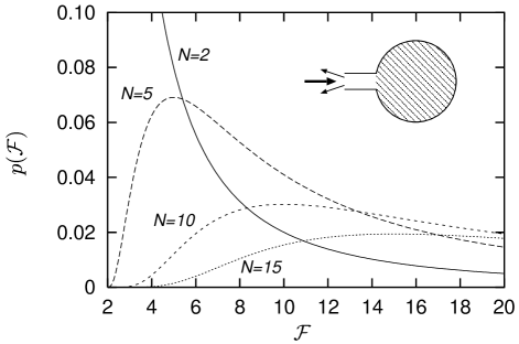
FIG. 4.: Probability distribution of the noise figure near the laser threshold for an amplifying disordered cavity, computed from Eq. (43) for $f=-1$. The most probable value is ${\cal F}=N$, while the average value diverges.

The distribution of ${\cal F}=-2f|u_{m_{0}}|^{-2}$ becomes

$$p({\cal F})=-2f(N-1)\left(1+\frac{2f}{{\cal F}}\right)^{N-2}{\cal F}^{-2}\;,$$ (43)

for $N\geq 2$ and ${\cal F}\geq-2f$. We have plotted $p({\cal F})$ in Fig. 4 for complete population inversion ($f=-1$) and several choices of $N$. It is a broad distribution, all its moments are divergent. The typical value of the noise figure is the value at which $p({\cal F})$ becomes maximal, hence

$${\cal F}_{\text{typ}}=-fN,\quad N\geq 2\;.$$ (44)

In the single-mode case, in contrast, ${\cal F}=-2f$ for every member of the ensemble [hence $p({\cal F})=\delta({\cal F}+2f)$]. We conclude that the typical value of the noise figure near the laser threshold of a disordered cavity is larger than in the single-mode case by a factor $N/2$.

VII Absorbing media

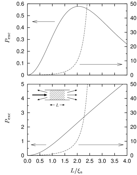
FIG. 5.: Excess noise power $P_{\text{exc}}$ for an absorbing (solid line, left axis) respectively amplifying disordered waveguide (dashed line, right axis), in units of $\alpha^{2}l|f|I_{0}/L$. The top panel is for detection in transmission, the bottom panel for detection in reflection.

The general theory of Sec. II can also be applied to an absorbing medium, in equilibrium at temperature $T>0$. Eq. (6) then has to be replaced with

$$a^{{\text{out}}}(\omega)=S(\omega)a^{{\text{in}}}(\omega)+Q(\omega)b(\omega)\;,$$ (45)

where the bosonic operator $b$ has the expectation value

$$\langle b_{n}^{\dagger}(\omega)b_{m}(\omega^{\prime})\rangle=\delta_{nm}\delta(\omega-\omega^{\prime})f(\omega,T)\;,$$ (46)

and the matrix $Q$ is related to $S$ by

$$QQ^{\dagger}={\openone}-SS^{\dagger}\;.$$ (47)

The formulas for $F(\xi)$ of Sec. III remain unchanged.

Ensemble averages for absorbing systems follow from the corresponding results for amplifying systems by substitution $\tau_{a}\to-\tau_{a}$. (This follows from a general duality theorem [17] between absorbing and amplifying systems.) The results for an absorbing disordered waveguide with detection in transmission are

$$\bar{I} = \frac{4\alpha l}{3L}I_{0}\frac{s}{\sinh s}\;,$$ (48)

$$P_{\text{exc}} = \frac{2\alpha^{2}l}{3L}fI_{0}s\left[\frac{3}{\sinh s}-\frac{2s+\,\text{cotanh}\,s}{\sinh^{2}s}\right.$$ (50)

$${}\left.\quad\mbox{}-\frac{s\,\text{cotanh}\,s-1}{\sinh^{3}s}+\frac{s}{\sinh^{4}s}\right]\;,$$

where $s=L/\xi_{a}$ with $\xi_{a}$ the absorption length. Similarly, for detection in reflection one has

$$\bar{I} = \alpha I_{0}\left[1-\frac{4l}{3L}s\,\text{cotanh}\,s\right]\;,$$ (51)

$$P_{\text{exc}} = \frac{2\alpha^{2}l}{3L}fI_{0}s\left[2\,\text{cotanh}\,s-\frac{1}{\sinh s}-\frac{\,\text{cotanh}\,s}{\sinh^{2}s}\right.$$ (53)

$${}\quad\left.\mbox{}-\frac{s\,\text{cotanh}\,s-1}{\sinh^{3}s}+\frac{s}{\sinh^{4}s}\right]\;.$$

These formulas follow from Eqs. (26)–(31) upon substitution of $s\to is$.

For an absorbing disordered cavity, we find [substituting $\gamma\to-\gamma$ in Eqs. (34)–(35)],

$$\bar{I} = \alpha I_{0}\frac{1}{1+\gamma}\;,$$ (54)

$$P_{\text{exc}} = 2\alpha^{2}fI_{0}\gamma\frac{\gamma^{2}+\gamma+1}{(1+\gamma)^{4}}\;,$$ (55)

with $\gamma$ the dimensionless absorption rate.

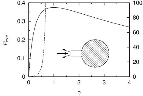
FIG. 6.: Excess noise power $P_{\text{exc}}$ for an absorbing (solid line, left axis) respectively amplifying disordered cavity (dashed line, right axis), in units of $\alpha^{2}|f|I_{0}$.

Since typically $f\ll 1$ in absorbing systems, the noise figure ${\cal F}$ is dominated by shot noise, ${\cal F}\approx I_{0}/\bar{I}$. Instead of ${\cal F}$ we therefore plot the excess noise power $P_{\text{exc}}$ in Figs. 5 and 6. In contrast to the monotonic increase of $P_{\text{exc}}$ with $1/\tau_{a}$ in amplifying systems, the absorbing systems show a maximum in $P_{\text{exc}}$ for certain geometries. The maximum occurs near $L/\xi_{a}=2$ for the disordered waveguide with detection in transmission, and near $\gamma=1$ for the disordered cavity. For larger absorption rates the excess noise power decreases because $\bar{I}$ becomes too small for appreciable beating with the spontaneous emission.

VIII Conclusion

In summary, we have studied the photodetection statistics of coherent radiation that has been transmitted or reflected by an amplifying or absorbing random medium. The cumulant generating function $F(\xi)$ is the sum of two terms. The first term is the contribution from spontaneous emission obtained in Ref. [6]. The second term $F_{\text{exc}}$ is the excess noise due to beating of the coherent radiation with the spontaneous emission. Equation (18) relates $F_{\text{exc}}$ to the transmission and reflection matrices of the medium.

In the applications of our general result for the cumulant generating function we have concentrated on the second cumulant, which gives the spectral density $P_{\text{exc}}$ of the excess noise. We have found that $P_{\text{exc}}$ increases monotonically with increasing amplification rate, while it has a maximum as a function of absorption rate in certain geometries.

In amplifying systems we studied how the noise figure ${\cal F}$ increases on approaching the laser threshold. Near the laser threshold the noise figure shows large sample-to-sample fluctuations, such that its statistical distribution in an ensemble of random media has divergent first and higher moments. The most probable value of ${\cal F}$ is of the order of the number $N$ of propagating modes in the medium, independent of material parameters such as the mean free path. It would be of interest to observe this universal limit in random lasers.

Derivation of Eq. (18)

To evaluate the Gaussian averages that lead to Eq. (18), it is convenient to use a matrix notation. We replace the summation in Eq. (12) by a multiplication of the vector $a^{\text{out}}$ with the projection ${\cal P}a^{\text{out}}$, where the projection matrix ${\cal P}$ has zero elements except ${\cal P}_{nn}=1$, $N+1\leq n\leq 2N$. We thus write

$$W=\alpha\int_{0}^{\tau}dt\,a^{{\text{out}}\dagger}(t){\cal P}a^{{\text{out}}}(t)\;.$$ (56)

Insertion of Eqs. (6) and (13) gives

$$W = \frac{\alpha}{2\pi}\int_{0}^{\tau}\!\!dt\int_{0}^{\infty}\!\!\!\!d\omega\int_{0}^{\infty}\!\!\!\!d\omega^{\prime}\!\left[a^{{\text{in}}\dagger}(\omega)S^{\dagger}(\omega)+c(\omega)V^{\dagger}(\omega)\right]$$ (58)

$$\times{\cal P}\left[S(\omega^{\prime})a^{{\text{in}}}(\omega^{\prime})+V(\omega^{\prime})c^{\dagger}(\omega^{\prime})\right]e^{i(\omega-\omega^{\prime})t}\;.$$

As explained in Sec. III we discretise the frequency as $\omega_{p}=p\Delta$, $p=1,2,3,\ldots$. The integral over frequency is then replaced with a summation,

$$\int_{0}^{\infty}d\omega\,g(\omega)\to\Delta\sum_{p=1}^{\infty}g(\omega_{p})\;.$$ (59)

We write Eq. (58) as a matrix multiplication,

$$\xi W={a}^{{\text{in}}\dagger}{A}{a}^{{\text{in}}}+{c}{B}{c}^{\dagger}+{a}^{{\text{in}}\dagger}{C}^{\dagger}{c}^{\dagger}+{c}{C}{a}^{{\text{in}}}\;,$$ (60)

with the definitions

$${A}_{np,n^{\prime}p^{\prime}} = \frac{\alpha\Delta\xi}{2\pi}\int_{0}^{\tau}dt\left(S^{\dagger}(\omega_{p}){\cal P}S(\omega_{p^{\prime}})\right)_{nn^{\prime}}e^{i\Delta(p-p^{\prime})t}\;,$$ (61)

$${B}_{np,n^{\prime}p^{\prime}} = \frac{\alpha\Delta\xi}{2\pi}\int_{0}^{\tau}dt\left(V^{\dagger}(\omega_{p}){\cal P}V(\omega_{p^{\prime}})\right)_{nn^{\prime}}e^{i\Delta(p-p^{\prime})t}\;,$$ (62)

$${C}_{np,n^{\prime}p^{\prime}} = \frac{\alpha\Delta\xi}{2\pi}\int_{0}^{\tau}dt\left(V^{\dagger}(\omega_{p}){\cal P}S(\omega_{p^{\prime}})\right)_{nn^{\prime}}e^{i\Delta(p-p^{\prime})t}\;,$$ (63)

$${a}^{{\text{in}}}_{np} = \Delta^{1/2}a^{{\text{in}}}_{n}(\omega_{p}),\qquad{c}_{np}=\Delta^{1/2}c_{n}(\omega_{p})\;.$$ (64)

We now apply the optical equivalence theorem [12], as discussed in Sec. III. The operators $a^{\text{in}}_{np}$ are replaced by constant numbers $\delta_{n{m_{0}}}\delta_{pp_{0}}(2\pi I_{0}/\Delta)^{1/2}$. The operators $c_{np}$ are replaced by independent Gaussian variables, such that the expectation value (14) takes the form of a Gaussian integral,

$$\langle:e^{\xi W}:\rangle=\int d\left\{{c}_{np}\right\}\exp\left[\xi W+\sum_{np}|c_{np}|^{2}/f(\omega_{p},T)\right]$$ (65)

$$=\int d\left\{{c}_{np}\right\}\exp\left[{a}^{{\text{in}}*}{A}{a}^{{\text{in}}}-{c}{M}{c}^{*}+{a}^{{\text{in}}*}{C}^{\dagger}{c}^{*}+{c}{C}{a}^{{\text{in}}}\right]\;,$$ (66)

where we have defined

$${M}_{np,n^{\prime}p^{\prime}}=-{B}_{np,n^{\prime}p^{\prime}}-\frac{\delta_{nn^{\prime}}\delta_{pp^{\prime}}}{f(\omega_{p})}\;.$$ (68)

We eliminate the cross-terms of ${a}^{{\text{in}}}$ and ${c}$ in Eq. (LABEL:Fxicomp2) by the substitution

$${c^{\prime}}^{*}={c}^{*}-{M}^{-1}{C}{a}^{{\text{in}}}\;,$$ (69)

leading to

$$\langle:e^{\xi W}:\rangle = \exp\left[{a}^{{\text{in}}*}({A}+{C}^{\dagger}{M}^{-1}{C}){a}^{{\text{in}}}\right]$$ (71)

$$\times\int d\left\{{c^{\prime}}_{np}\right\}\exp\left(-{c^{\prime}}{M}{c^{\prime}}^{*}\right)\;.$$

The integral is proportional to the determinant of ${M}^{-1}$, giving the generating function

$$F(\xi) = \mbox{constant}-\ln\|{M}\|+{a}^{{\text{in}}*}\left({A}+{C}^{\dagger}{M}^{-1}{C}\right){a}^{{\text{in}}}$$ (72)

$$= \mbox{constant}-\ln\|{M}\|$$ (74)

$$\mbox{}+\frac{2\pi I_{0}}{\Delta}\left({A}+{C}^{\dagger}{M}^{-1}{C}\right)_{{m_{0}}p_{0},{m_{0}}p_{0}}\;.$$

The additive constant follows from $F(0)=0$. The term $-\ln\|{M}\|$ is the contribution from amplified spontaneous emission calculated in Ref. [6]. The term proportional to $I_{0}$ is the excess noise of the coherent radiation, termed $F_{\text{exc}}$ in Sec. III.

Eq. (74) can be simplified in the long-time regime, $\omega_{c}\tau\gg 1$. We may then set $\Delta=2\pi/\tau$ and use

$$\int_{0}^{\tau}e^{i\Delta(p-p^{\prime})t}dt=\tau\delta_{pp^{\prime}}\;.$$ (75)

The matrices defined in Eq. (64) thus become diagonal in the frequency index,

$${A}_{np,n^{\prime}p^{\prime}}=\frac{\alpha\Delta\tau\xi}{2\pi}\left(S^{\dagger}(\omega_{p}){\cal P}S(\omega_{p})\right)_{nn^{\prime}}\delta_{pp^{\prime}}$$ (76)

and similarly for ${B}$ and ${C}$. We then find

$$(A+C^{\dagger}M^{-1}C)_{np,n^{\prime}p^{\prime}}=$$ (78)

$$\mbox{~{}~{}~{}~{}~{}~{}~{}}\frac{\alpha\xi\Delta\tau}{2\pi}(S^{\dagger}{\cal P}[{\openone}+\alpha\xi fVV^{\dagger}{\cal P}]^{-1}S)_{nn^{\prime}}\delta_{pp^{\prime}}\;,$$

where $f$, $S$, and $V$ are evaluated at $\omega=\omega_{p}$. Substitution into Eq. (74) gives the result (18) for $F_{\text{exc}}(\xi)$.

Simplification of Eq. (74) is also possible in the short-time regime, when $\Omega_{c}\tau\ll 1$, with $\Omega_{c}$ the frequency range over which $SS^{\dagger}$ differs appreciably from the unit matrix. The generating function then is

$$F_{\text{exc}}(\xi)=\alpha\xi\tau I_{0}\biggl{(}t^{\dagger}(\omega_{0})\Bigl{[}{\openone}-\frac{\alpha\xi\tau}{2\pi}\int_{0}^{\infty}d\omega f(\omega,T)$$ (79)

$$\times\left({\openone}-r(\omega)r^{\dagger}(\omega)-t(\omega)t^{\dagger}(\omega)\right)\Bigr{]}^{-1}t(\omega_{0})\biggr{)}_{{m_{0}}{m_{0}}}\!\!\!\;.$$ (80)

REFERENCES

- [1] C. H. Henry and R. F. Kazarinov, Rev. Mod. Phys. 68, 801 (1996).
- [2] C. M. Caves, Phys. Rev. D 26, 1817 (1982).
- [3] J. R. Jeffers, N. Imoto, and R. Loudon, Phys. Rev. A 47, 3346 (1993).
- [4] R. Matloob, R. Loudon, M. Artoni, S. Barnett, and J. Jeffers, Phys. Rev. A 55, 1623 (1997).
- [5] D. Wiersma and A. Lagendijk, Physics World, January 1997, p. 33.
- [6] C. W. J. Beenakker, Phys. Rev. Lett. 81, 1829 (1998).
- [7] C. W. J. Beenakker, Rev. Mod. Phys. 69, 731 (1997).
- [8] R. Matloob, R. Loudon, S. M. Barnett, and J. Jeffers, Phys. Rev. A 52, 4823 (1995).
- [9] T. Gruner and D.-G. Welsch, Phys. Rev. A 54, 1661 (1996).
- [10] R. J. Glauber, Phys. Rev. Lett. 10, 84 (1963).
- [11] P. L. Kelley and W. H. Kleiner, Phys. Rev. 136, A316 (1964).
- [12] L. Mandel and E. Wolf, Optical Coherence and Quantum Optics (Cambridge University Press, New York, 1995).
- [13] P. A. Mello and S. Tomsovic, Phys. Rev. B 46, 15963 (1992).
- [14] P. W. Brouwer, Phys. Rev. B 57, 10526 (1998). The formulas in this paper refer to an absorbing slab. For an amplifying slab one should replace by . Note that Equation (13c) contains a misprint: The second and third term between brackets should have, respectively, signs minus and plus instead of plus and minus.
- [15] C. W. J. Beenakker, in Diffuse Waves in Complex Media, NATO ASI Series, edited by J. P. Fouque (Kluwer, Dordrecht, 1999).
- [16] P. Pereyra and P. A. Mello, J. Phys. A: Math. Gen. 16, 237 (1983).
- [17] J. C. J. Paasschens, T. S. Misirpashaev, and C. W. J. Beenakker, Phys. Rev. B 54, 11887 (1996).