The linewidth of a non-Markovian atom laser

Abstract

We present a fully quantum mechanical treatment of a single mode atom laser including pumping and output coupling. By ignoring atom-atom interactions, we have solved this model without making the Born-Markov approximation. We find substantially less gain narrowing than is predicted under that approximation.

An atom laser is a device which produces a coherent atomic de Broglie wave analogous to the coherent light wave produced by an optical laser. Unlike optical lasers, existing experimental atom lasers are not pumped [1, 2]. Consequently they do not exhibit gain narrowing, the phenomenon whereby the output linewidth is much narrower above threshold than below threshold.

Atom laser models based on the Born-Markov approximations (BMA) predict gain narrowing, but they fail for a range of physically interesting parameter regimes [3, 4, 5]. In the BMA a laser, optical or atom, is described by a quantum optical master equation [6]. In the simplest case this models an oscillator subject to gain and loss, due to pumping and output coupling respectively. The linewidth is associated with the net dissipation in the system, which is the difference between the gain and loss. This difference decreases as the laser is pumped above threshold, giving rise to the gain-narrowed laser linewidth. This idealised Schawlow-Townes linewidth has its fundamental origin in spontaneous-emission-driven phase diffusion [7]. By analogy, Graham [8] has estimated the ultimate atom laser linewidth due to scattering of thermally excited phonons. Previous studies based on the BMA have shown that certain pumping processes, such as evaporative cooling, severely broaden the atom laser linewidth beyond this fundamental limit [9, 10].

In the following we present a quantum mechanical analysis of the atom laser which does not make the BMA. We find that the gain narrowing is several orders of magnitude less than predicted using the BMA. Our methods may be useful for other non-Markovian systems, such as spontaneous emission in optical band-gap materials [11].

Models based on the nonlinear Schrödinger equation are able to include interatomic interactions [12, 13, 14, 15]. However they implicitly assume that the lasing field is in a coherent state, which makes it impossible to calculate the linewidth of the resulting output, since no information remains about the quantum statistics. Interatomic interactions are difficult to include in a full quantum mechanical model, so our model assumes that they are negligible. This is an accurate description of very dilute systems.

We have previously shown that a simple model of atom laser output coupling produces a nondispersing state which prevents a pumped atom laser from reaching a steady state [5]. Adding gravity destroyed the non-dispersing state, overcoming the problem. Hence the atom laser modeled in this paper includes the effect of gravity on the output atom field.

We model the atom laser by separating it into three parts. The lasing mode is an atomic cavity with large energy level separation. We assume that the cavity is single mode, with annihilation operator $a$ and a Hamiltonian $H_{s}$. The external atomic field has a different electronic state, so the atoms are no longer affected by the trapping potential. We model the external modes with the field operator $\psi(x)$ and the Hamiltonian $H_{o}$. The operators $a$ and $\psi(x)$ satisfy the normal boson commutation relations. The pump reservoir is coupled to the cavity by an irreversible process. At this stage, we will describe the pump by the Hamiltonian $H_{p}$, which also couples the atoms from a pump reservoir into the system mode. The coupling between the lasing mode and the output modes is

$$H_{int}=-i\hbar\left(\xi(t)\;a_{I}^{{\dagger}}(t)-\xi^{{\dagger}}(t)\;a_{I}(t)\right),$$ (1)

where we have introduced the interaction picture operators

$$\xi(t) = \int dx\;\kappa(x)\psi_{I}(x,t),$$ (2)

$$\psi_{I}(x,t) = e^{iH_{o}(t-t_{0})/\hbar}\;\psi(x,t_{0})\;e^{-iH_{o}(t-t_{0})/\hbar},$$ (3)

$$a_{I}(t) = e^{i/\hbar(H_{s}+H_{p})(t-t_{0})}\;a(t_{0})\;e^{-i/\hbar(H_{s}+H_{p})(t-t_{0})}.$$ (4)

The shape of the coupling $\kappa(x)$ is determined largely by the spatial wavefunction of the laser mode.

Using the unitary evolution operator corresponding to the interaction Hamiltonian Eq.(1), we find in the Heisenberg picture,

$$\psi_{H}(x,t)=\psi_{I}(x,t)-\int_{t_{0}}^{t}ds\;F(x,t,s)a_{H}(s),$$ (5)

where $\psi_{H}(x,t)$ and $a_{H}(t)$ are Heisenberg operators, and

$$F(x,t,s) = [\psi_{I}(x,t),\xi^{{\dagger}}(s)]$$ (6)

$$= \int dy\;\kappa^{*}(y)[\psi_{I}(x,t),\psi_{I}^{{\dagger}}(y,s)]$$ (7)

$$= \int dy\;\kappa^{*}(y)G(x,t,y,s)$$ (8)

where $G(x,t,y,s)$ is the Green’s function propagator due to the output Hamiltonian, $H_{o}$, only. These functions can be written in closed form for several useful cases, including free space, free space with gravity, and a repulsive Gaussian potential. We may use Eq. (5) to calculate any observable of the output field, providing we know the complete history of the system, $a_{H}(s)$.

To calculate the output energy flux we transform our interaction Hamiltonian into the basis of the energy eigenstates of the output modes: $H_{o}=\int dp\;\hbar\>\omega_{p}c_{p}^{{\dagger}}c_{p}$, where $c_{p}$ is the annihilation operator associated with the eigenstate of $H_{o}$ that has a position space wavefunction $u_{p}(x)$ and energy $\hbar\omega_{p}$. Defining $\bar{\kappa}(p)=\int dx\;u_{p}(x)\>\kappa(x)$, the output energy flux in terms of the two time correlation of the system is

$$\frac{d\langle c_{p}^{{\dagger}}c_{p}\rangle}{dt}=2\;|\bar{\kappa}(p)|^{2}\;\Re{\left(\int_{0}^{t}ds\;e^{-i\omega_{p}\Delta t}\langle a^{{\dagger}}(t)a(s)\rangle\right)},$$ (9)

where $\Re$ denotes the real part, and $\Delta t=t-s$. This assumes that at time $t=0$, the output field was in the vacuum state.

When the output field is in free space and the only term in $H_{o}$ is the kinetic energy, then the eigenstates are the momentum eigenstates. In this case, $\bar{\kappa}(p)$ is just the Fourier transform of $\kappa(x)$. When there is a gravitational field, the eigenstates are Airy functions with a displacement which depends on the energy:

$$u_{p}(x)={\cal N}Ai[\beta(x-\hbar\omega_{p}/(mg))]$$ (10)

where $\mathcal{N}$ is a normalisation constant, the length scale is given by $\beta=(2m^{2}g/\hbar^{2})^{1/3}$, and $m$ is the atomic mass. In this case $\bar{\kappa}(p)$ must be calculated numerically.

Following Scully and Lamb we model pumping by the injection of a Poissonian sequence of excited atoms into the atom laser [6, 16]. These atoms may spontaneously emit a photon and make a transition either into the atom lasing mode or into other modes of the lasing cavity. For simplicity, we consider a two-mode approximation. To obtain the pumping term, we consider the effect of a single atom injected into the atom laser, and then extend this to describe the effect of a distribution of atoms. This gives the master equation [17]

$$\left(\dot{\rho}\right)_{\mbox{pump}} = r{\cal D}[a^{{\dagger}}]\left(n_{s}+{\cal A}[a^{{\dagger}}]\right)^{-1}\rho,$$ (11)

where $r$ is the rate at which atoms are injected into the cavity, and $n_{s}$ the saturation number. The superoperators ${\cal D}$ and ${\cal A}$ are defined by

$${\cal D}[c] = c\rho c^{{\dagger}}-{\cal A}[c],$$ (12)

$${\cal A}[c]\rho = \frac{1}{2}(c^{{\dagger}}c\rho+\rho c^{{\dagger}}c).$$ (13)

In our particular model $n_{s}$ depends on the ratio of the probability that an atom will spontaneously emit into the lasing mode to the probability that the atom will emit into another mode.

If we make the Born approximation, trace over the output modes, and then make the Markov approximation, we can write the damping term of the master equation as [5]

$$\left(\dot{\sigma}\right)_{\mbox{damp}} = \gamma_{BM}{\cal D}[a]\sigma,$$ (14)

where $\gamma_{BM}$ is related to the above threshold mean atom number $\bar{n}$ and saturation photon number $n_{s}$ by

$$\gamma_{BM}=r/(\bar{n}+n_{s}).$$ (15)

The full equation of motion is then

$$\frac{d\langle a^{{\dagger}}\rangle}{dt} = \left(P-\frac{\gamma_{BM}}{2}\right)\langle a^{{\dagger}}\rangle\approx-\frac{r}{4\bar{n}^{2}}\langle a^{{\dagger}}\rangle,$$ (16)

$$P \approx r/\{2(\bar{n}+n_{s})+1\},$$ (17)

which has an error term proportional to $r/\bar{n}^{3}$ if we assume that the system is close to a coherent state. The solution to this equation is an exponential decay, and the energy spectrum is therefore Lorentzian, with a width of

$$\Gamma_{BM}=r/(4\bar{n}^{2}).$$ (18)

If we do not make the Born or Markov approximations, but we do assume that the trap population is localised around some (at this stage unknown) value $\bar{n}$, we find

$$\frac{\partial}{\partial t}\ \langle a^{{\dagger}}(t)\rangle=(i\omega_{o}+P)\langle a^{{\dagger}}(t)\rangle+\int dx\;\kappa^{*}(x)\langle\psi^{{\dagger}}_{x,t}\rangle$$ (19)

well above threshold. Note that we can no longer relate $\bar{n}$ directly to the physical parameters of the problem using Eq.(15), which has used the Born approximation. Since $P$ determines $n_{s}$, we seek an iterative method to produce a self-consistent solution.

Under our assumptions the pumping is effectively linear, so we may use the quantum regression theorem. Using Eq.(5), we may derive the following Volterra convolution type integro-differential equation for the two time correlation function:

$$\frac{\partial}{\partial\tau} \langle a^{{\dagger}}(t+\tau)a(t)\rangle=(i\omega_{o}+P)\langle a^{{\dagger}}(t+\tau)a(t)\rangle$$ (20)

$$\>\>\>\;\;\;-\int_{0}^{t+\tau}du\;f^{*}(t+\tau-u)\langle a^{{\dagger}}(u)a(t)\rangle,$$ (21)

where $\tau>0$, and $f(\Delta t)$ is the memory function

$$f(\Delta t)=\int dx\;\kappa(x)F(x,\Delta t).$$ (22)

We have assumed that $F(x,t,s)$ is a function of $\Delta t=t-s$. This again assumes that at time $t=0$, the output field was in the vacuum state. This equation is not sufficient to specify the dynamics of the cavity, as it is only a single partial integro-differential equation in a two dimensional space. We also require the integro-differential equation for the intracavity number, which we can generate in a similar manner. Well above threshold, we obtain

$$\frac{d}{dt}\langle a^{{\dagger}}a\rangle(t)=r\\ -\int_{0}^{t}ds\;2\Re\{f^{*}(\Delta t)\langle a^{{\dagger}}(s)a(t)\rangle\}.$$ (23)

These equations are difficult to solve in general, but can be solved in various limits. For example, if the kernel $f(t)$ is a $\delta$-function, as in the broadband limit of the optical laser, then the equations would become local, and the solution is an exponential. Although the broadband limit can be a good approximation for the atomic case as well [4], in general the atoms will disperse, which gives the system an irreducible memory.

In order to produce analytical forms for the memory functions we assume that the coupling is Gaussian, and that there is no net momentum kick given to the atoms:

$$\kappa(x)=\sqrt{\gamma}\left(2\sigma_{k}^{2}/\pi\right)^{1/4}\exp[-(\sigma_{k}\;x)^{2}],$$ (24)

where $\hbar\sigma_{k}$ is the momentum width of the coupling and $\gamma$ is the strength of the coupling. In the presence of a gravitational field, $V=mgx$, the Green’s function in Eq.(8) can be found as a standard result [18, 19]:

$$G(x,t,y,s)=\sqrt{\frac{1}{4\pi i\lambda\Delta t}}\times$$ (25)

$$\;\;\;\exp[({\frac{i(x-y)^{2}}{4\lambda\Delta t}-\frac{ig\Delta t(x+y)}{4\lambda}-\frac{ig^{2}\Delta t^{3}}{48\lambda}})],$$ (26)

where $\lambda=\hbar/(2m)$, and $\Delta t=t-s$. This leads to the following form for the memory function,

$$f(\Delta t)=\frac{\gamma\;\;\exp({-\frac{g^{2}\>\Delta t^{2}}{32\>\lambda^{2}\>\sigma_{k}^{2}}})\;\;\exp({\frac{-i\>g^{2}\>\Delta t^{3}}{48\>\lambda}})}{\sqrt{1+2\>i\>\lambda\>\Delta t\>\sigma_{k}^{2}}}.$$ (27)

For coupling into free space, $g=0$, and $f(\Delta t)$ goes as $1/\sqrt{\Delta t}$ in the long time limit. There are no useful approximations when $g\neq 0$. This is because the broadband limit of the integrals involving $f(\Delta t)$ become unbounded in amplitude, and their convergence is due to their highly oscillatory nature.

Eq. (21) and Eq. (23) do not form a standard pair of partial integro-differential equations. The derivative in Eq. (21) is only defined for $\tau>0$, and so we cannot require that the solution obey this equation through the whole domain of the integral. This means that Eq. (21) cannot be integrated to find the solution, as we do not actually know the derivative at any point. Since the two-time correlation is Hermitian, we can we rewrite the integral so that the domain remains in the $\tau>0$ plane, but we still do not have a continuously defined derivative along the length of the integral.

We proceed by making an ansatz which uses the solution of Eq. (21) which has been extended into the region $\tau<0$. We then use the $\tau>0$ portion of this solution to substitute into the two time correlation in Eq. (23). We introduce the function $J(t)$, which is the solution of the equation

$$\frac{dJ(t)}{dt}=(i\omega_{o}+P)J(t)-\int_{0}^{t}ds\;f^{*}(\Delta t)J(s).$$ (28)

This means that

$$\langle a^{{\dagger}}(t+\tau)a(t)\rangle=\langle a^{{\dagger}}a\rangle(t)J(t+\tau)/J(t)$$ (29)

is a solution of Eq. (21) with the correct initial condition at $\tau=0$. We then substitute this result into Eq.(23):

$$\frac{d\langle a^{{\dagger}}a\rangle(t)}{dt}=r-\int_{0}^{t}ds\;\langle a^{{\dagger}}a\rangle(s)\;\Re{\left(\frac{2f(\Delta t)J(t)}{J(s)}\right)}.$$ (30)

Solving these two equations gives the two time correlation for the lasing mode, from which we may find the properties of the output field. It is only consistent with our linearisation of the pumping if the number of atoms in the trap, $\bar{n}$, converges to the value which originally produced the parameter $P$. Since we require $P$ to generate the solution, and $\bar{n}$ is simply the long time limit of Eq. (30), the effective free parameter is $n_{s}$. This threshold parameter must be much smaller than $\bar{n}$, so we search for a value of $P$ which gives the result $\bar{n}\gg n_{s}$.

Once it is established that Eq. (30) is approaching a stable steady state, a fast way of finding it is to set the derivative to zero, and assume that $\langle a^{{\dagger}}a\rangle(s)=\bar{n}$ over the support of the kernel. This gives

$$\bar{n}=r\left(\int_{0}^{t}ds\;\Re\left(\frac{2f(\Delta t)J(t)}{J(s)}\right)\right)^{-1}.$$ (31)

We transform Eq. (28) into a rotating frame by introducing the function $N(t)=J(t)\;\exp(-i\omega_{o}t-Pt)$ and rewriting it in terms of $N(t)$:

$$\frac{dN(t)}{dt}=-\int_{0}^{t}ds\;H(\Delta t)N(s)$$ (32)

where $H(\Delta t)=f^{*}(\Delta t)\exp(-[i\omega_{o}+P]\Delta t)$. An effective numerical method for solving this equation is direct integration using a second-order algorithm for both the integration and the calculation of the integral to find the derivative at each timestep [20].

We now calculate the output properties of an atom laser. We use the trap frequency $\omega_{o}=2\pi\times 123$ Hz [1], an atomic mass of $m=5\times 10^{-26}$kg, a gravitational acceleration of $g=9.8\sin(0.18)$ m s^-2, and the coupling given by Eq. (24) with a momentum width $\sigma_{k}=4.4\times 10^{5}$ m^-1. We use a damping constant of $\gamma=2.0\times 10^{4}s^{-2}$, and a threshold of $n_{s}=47$. As the pumping rate $r$ increases, the steady state number of atoms in the cavity $\bar{n}$ increases, and the modulus of the two time correlation decays more slowly. The energy spectrum of the output flux is proportional to the Fourier transform of the two time correlation through Eq. (9), so the laser shows gain narrowing.

In Table 1 we show the results of these calculations. The linewidth of the output flux, $\Gamma$, is calculated directly from the two time correlation using Eq. (9). This is compared to the linewidth given by the Born-Markov approximation $\Gamma_{BM}$, Eq. (18).

The atom laser linewidth predicted by our theory is several orders of magnitude larger than that predicted using the BMA result. We plot the spectral flux corresponding to three of these pumping rates in Fig. 1. The vertical scale is normalised to the peak height for each plot so that the width of the spectra can be easily compared. The spectra are almost Lorenztian, but have a drastically different width and are slightly shifted compared to the results under the BMA.

Our model does not include atom-atom interactions, and therefore only works when the atomic field is very dilute. The advantage of our model is that, unlike mean field models, we have avoided making the approximation that the lasing mode is perfectly coherent. Future work will involve generalising this atom laser model to include atom-atom interactions.

This work was supported by the Australian Research Council. J.H. would like to thank M.Jack, T.Ralph, H.Wiseman and M.Naraschewski for their helpful discussions.

TABLE I.: Linewidths and cavity atom number as a function of pumping rate $r$.

$r$ ($10^{3}$/s)	$\bar{n}$	$\Gamma$($s^{-1}$)	$\Gamma_{BM}$($s^{-1}$)
20	450	2.1	0.025
40	910	1.1	0.012
80	1800	0.56	0.0062
800	$1.8\times 10^{4}$	0.035	0.00062

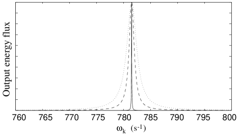
FIG. 1.: The spectra of the output energy flux for three different pumping rates. The dotted, dashed and solid lines represent $r=40s^{-1}$, $r=80s^{-1}$ and $r=800s^{-1}$ respectively. Other parameters are given in the text.

REFERENCES

- [1] M.-O. Mewes et al., Phys. Rev. Lett.78, 582 (1997), M.R. Andrews et al., Science 275, 637 (1997).
- [2] B.P. Anderson and M.A. Kasevich, Science 282, 1686 (1998).
- [3] J. Hope, Phys. Rev. A55, R2531 (1997).
- [4] G.M. Moy and C.M. Savage, Phys. Rev. A56, R1087 (1997).
- [5] G.M. Moy, J.J. Hope and C.M. Savage, Phys. Rev. A59, 667 (1999).
- [6] D.F. Walls and G.J. Milburn, Quantum Optics, Springer-Verlag (1994).
- [7] A.L. Schawlow and C.H. Townes, Phys. Rev. 112, 1940 (1958).
- [8] R. Graham, Phys. Rev. Lett.81, 5262 (1998).
- [9] H.M. Wiseman and M.J. Collett, Physics Lett. A 202, 246 (1995).
- [10] H.M. Wiseman, A. Martins and D.F. Walls, Quantum Semiclass. Opt. 8, 737 (1996).
- [11] N. Vats and S. John, Phys. Rev. A58, 4168 (1998).
- [12] M. Naraschewski, A. Schenzle, and H. Wallis, Phys. Rev. A, 56, 603 (1997).
- [13] H. Steck, M. Naraschewski and H. Wallis, Phys. Rev. Lett.80, 1 (1998).
- [14] W. Zhang and D.F. Walls, Phys. Rev. A57, 1248 (1998).
- [15] B. Kneer et al., Phys. Rev. A58, 4841 (1998).
- [16] M.O. Scully and W.E. Lamb, Phys. Rev. A159, 208 (1967).
- [17] H. Wiseman, Phys. Rev. A, 56, 2068 (1997).
- [18] M.W. Jack, M. Naraschewski, M.J. Collett and D.F. Walls, unpublished.
- [19] see e.g. L.Schulman, Techniques and Applications of Path Integration, Wiley (1981).
- [20] see, for example, Numerical Recipes, which can be found at http://www.nr.com