Non Thermal Equilibrium States of Closed Bipartite Systems

Abstract

We investigate a two-level system in resonant contact with a larger environment. The environment typically is in a canonical state with a given temperature initially. Depending on the precise spectral structure of the environment and the type of coupling between both systems, the smaller part may relax to a canonical state with the same temperature as the environment (i.e. thermal relaxation) or to some other quasi equilibrium state (non thermal relaxation). The type of the (quasi) equilibrium state can be related to the distribution of certain properties of the energy eigenvectors of the total system. We examine these distributions for several abstract and concrete (spin environment) Hamiltonian systems, the significant aspect of these distributions can be related to the relative strength of local and interaction parts of the Hamiltonian.

I Introduction

In a composite but closed quantum system in which a smaller central system S is weakly coupled to a larger environment C, most of the (pure) states of the total system for a given energy (and possibly some additional constraints) exhibit properties of thermal equilibrium states with respect to the smaller part Gemmer et al. (2004), i.e. there exists a so-called dominant region in Hilbert space in which the entropy of the central system is close to its maximum value under the given constraints. Therefore for most pure initial states of the total system, the state of the central system shows decoherence and some kind of thermalization; it typically approaches a quasi-equilibrium canonical state with a temperature given by the spectral properties of the environment Borowski et al. (2003).

If the environment initially is in a thermal state with a given temperature and consists of many bands or of a broad continuum of levels, the central system typically relaxes to a thermal state with the same temperature. This type of relaxation will be called thermal relaxation in the following. Here we investigate to what extent certain structures of the total system influence the reached (quasi) equilibrium state. We will relate this equilibrium state to the distribution of the energy eigenvectors of the system, or rather certain important aspects of this distribution. We will show that there is a close relation between the two, and how this affects the equilibrium state for different system structures.

We particularly focus on a single spin-$1/2$ particle coupled to an environment of spin-$1/2$ particles. Recently, the properties of spin systems of different structure (rings, stars, and others) have been subject of extensive interest. A lot of work has been done on the question of entanglement Briegel and Raussendorf (2001); O’Connor and Wootters (2001); Wang (2002); Hutton and Bose (2004a, b); Vidal et al. (2003), their relaxation behavior has been addressed Breuer et al. (2004); Lages et al. (2004) and various techniques were suggested to make any spin interact with any other spin Imamoḡlu et al. (1999); Makhlin et al. (1999).

Here we extend our analysis form our previous paper Schmidt and Mahler (2005) regarding the controllability of relaxation behavior within these spin systems

II Canonical and Non Canonical Relaxation

Figure 1: A two-level system S in contact with an environment C consisting of two highly degenerate levels $k$, $k^{\prime}$ with degeneracies $g_{k}$, $g_{k^{\prime}}$.

Figure 1 shows a two-level system (TLS) in resonant ($\delta_{\text{S}}=\delta_{\text{C}}=\delta$) contact with an environment consisting of two “energy bands” $k$, $k^{\prime}$ of degeneracies $g_{k}$, $g_{k^{\prime}}$, respectively (for simplicity we use $g=g_{k}$, $g^{\prime}=g_{k^{\prime}}$ in the following, typically $g^{\prime}>g$). The coupling is assumed to be weak, the total system is described by the Hamiltonian

$$\hat{H}=\hat{H}_{\text{S}}+\hat{H}_{\text{C}}+\hat{H}_{\text{int}}.$$

A non equilibrium state $\mathinner{\lvert 1\rangle}_{\text{S}}\otimes\mathinner{\lvert\phi_{k}\rangle}_{\text{C}}$ is depicted (here $\mathinner{\lvert\phi_{k}\rangle}$ denotes an arbitrary pure environmental state in band $k$).

If this state is taken as the initial state of a Schrödinger time evolution of the total system, a relaxation to an equilibrium situation is expected in which the time-averaged reduced state operator of S is given by Gemmer et al. (2004)

$$\hat{\rho}_{\text{S}}=\frac{1}{g+g^{\prime}}\bigl{(}g^{\prime}\mathinner{\lvert 0\rangle}\!\mathinner{\langle 0\rvert}+g\mathinner{\lvert 1\rangle}\!\mathinner{\langle 1\rvert}\bigr{)}$$ (1)

which can be interpreted as a canonical state operator with inverse temperature

$$\beta_{\text{S}}=\frac{1}{k_{\text{B}}T}=\frac{1}{\delta_{\text{S}}}\ln\frac{g^{\prime}}{g}.$$

For a finite environment and weak random coupling, the reduced state of the central system after relaxation still fluctuates around (1), see Borowski et al. (2003).

If the central system relaxes to state (1) for any pure state $\mathinner{\lvert\phi_{k}\rangle}$ of the environment in band $k$, it will relax to the same state for an initial state in which the environment is completely mixed within band $k$, $\hat{\rho}_{0}=\mathinner{\lvert 1\rangle}\!\mathinner{\langle 1\rvert}\otimes\frac{\hat{1}_{k}}{g}$. $\hat{1}_{k}$ denotes the projector onto band $k$ of the environment.

Assume now that the environment is given by a large number $N$ of two level systems with a homogeneous Zeeman splitting, $\hat{H}_{\text{C}}=\sum_{i=1}^{N}\delta\hat{\sigma}_{z}^{(i)}$. The environment initially is taken to be in a thermal state of temperature $\beta_{\text{C}}$,

$$\hat{\rho}_{0}=\mathinner{\lvert 1\rangle}\!\mathinner{\langle 1\rvert}\otimes\frac{1}{Z}\,\mathrm{e}^{-\beta_{\text{C}}\hat{H}_{\text{C}}}.$$

If each band of the environment separately leads to a relaxation into a state (1), the equilibrium state of the central system is given by the canonical state with $\beta_{\text{S}}=\beta_{\text{C}}$ for large $N$. For finite $N$, the population of the excited state of S after relaxation is given by

$$(\hat{\rho}_{\text{S}})_{11}=\frac{N}{N+1}\frac{1}{1+\mathrm{e}^{\delta\beta_{\text{C}}}}+\frac{1}{N+1}\;\xrightarrow[N\gg 1]{}\;\frac{1}{1+\mathrm{e}^{\delta\beta_{\text{C}}}}.$$

Because of this we call the relaxation from an initial state $\mathinner{\lvert 1\rangle}_{\text{S}}\otimes\mathinner{\lvert\phi_{k}\rangle}_{\text{C}}$ to the reduced equilibrium state (1) canonical or thermal throughout this text.

However, not all environments lead to canonical relaxation of the central system. In Schmidt and Mahler (2005) we examined several types of spin environments and showed that many of these lead to an equilibrium state that differs from (1). We call these deviations non canonical or non thermal. Figure 2 shows the relaxation behavior for different types of environments. Obviously, not all relax to the same quasi equilibrium state.

Figure 2: $z$-component of the Bloch vector of S for the initial state depicted in figure 1. The environment consists of spins, curves are for different types of intra-environmental coupling. Fluctuations are due to the finite size of the system. The black line indicates canonical equilibrium.

III Energy Eigenvector Distributions

We now correlate deviations from canonical relaxation with the distribution of the energy eigenvectors of the total system. We only consider the situation depicted in figure 1, since environments with more bands in a canonical state can simply be derived from these results. As long as the interaction is weak relative to the band splitting, the total system can be reduced to the subspace consisting of the “cross states”

$$\{{\mathinner{\lvert 0_{\text{S}},\text{environment in band }k^{\prime}\rangle}},\quad$$

$$\quad\mathinner{\lvert 1_{\text{S}},\text{environment in band }k\rangle}\}.$$ (2)

In the following we will always refer only to this $(g+g^{\prime})$-dimensional subspace.

Instead of the temperature we consider the population inversion $\operatorname{Tr}\{\hat{\sigma}_{z}\hat{\rho}_{\text{S}}\}$ of the central system for mathematical convenience. The inversion of the canonical state (1) is given by

$$\mathinner{\langle\hat{\sigma}_{z}\rangle}_{\text{can}}=\frac{g-g^{\prime}}{g+g^{\prime}}.$$

The energy eigenvectors can be written in the form

$$\mathinner{\lvert\varepsilon\rangle}\approx\alpha_{\varepsilon}\mathinner{\lvert 0,\chi_{\varepsilon}\rangle}+\beta_{\varepsilon}\mathinner{\lvert 1,\eta_{\varepsilon}\rangle},$$ (3)

where $\mathinner{\lvert\chi_{\varepsilon}\rangle}$ is a state in band $k^{\prime}$, and $\mathinner{\lvert\eta_{\varepsilon}\rangle}$ a state in band $k$ of the environment. In the following we will use $\varepsilon$ as a discrete index running from $1$ to $g+g^{\prime}$ to number the energy eigenvectors within the subspace of Hilbert space spanned by the states (2).

We expand the initial state $\hat{\rho}_{0}=\mathinner{\lvert 1\rangle}\!\mathinner{\langle 1\rvert}\otimes\frac{\hat{1}_{k}}{g}$ in terms of these eigenvectors, $\hat{\rho}_{0}=\sum_{\varepsilon,\varepsilon^{\prime}}\rho_{0,\varepsilon\varepsilon^{\prime}}\mathinner{\lvert\varepsilon\rangle}\!\mathinner{\langle\varepsilon^{\prime}\rvert}$. Averaging over all times and tracing out the environment yields the equilibrium state of the central system,

$$\bar{\rho}_{\text{S}} =\sum_{\varepsilon}\rho_{0,\varepsilon\varepsilon}\operatorname{Tr}_{\text{C}}\bigl{\{}\mathinner{\lvert\varepsilon\rangle}\!\mathinner{\langle\varepsilon\rvert}\bigr{\}}$$

$$=\sum_{\varepsilon}\lvert\beta_{\varepsilon}\rvert^{2}\bigl{(}\lvert\alpha_{\varepsilon}\rvert^{2}\mathinner{\lvert 0\rangle}\!\mathinner{\langle 0\rvert}+\lvert\beta_{\varepsilon}\rvert^{2}\mathinner{\lvert 1\rangle}\!\mathinner{\langle 1\rvert}\bigr{)}.$$

The respective inversion is

$$\mathinner{\langle\bar{\sigma}_{z}\rangle}=\sum_{\varepsilon}\lvert\beta_{\varepsilon}\rvert^{2}\bigl{(}\lvert\beta_{\varepsilon}\rvert^{2}-\lvert\alpha_{\varepsilon}\rvert^{2}\bigr{)}.$$

We notice that

$$\lambda_{\varepsilon}=\lvert\beta_{\varepsilon}\rvert^{2}-\lvert\alpha_{\varepsilon}\rvert^{2}$$ (4)

is the inversion of $\mathinner{\lvert\varepsilon\rangle}$. Since $\lvert\beta_{\varepsilon}\rvert^{2}+\lvert\alpha_{\varepsilon}\rvert^{2}=1$ we can rewrite the time-averaged inversion of the central system completely in terms of the $\lambda_{\varepsilon}$’s,

$$\mathinner{\langle\bar{\sigma}_{z}\rangle}=\frac{1}{2}\biggl{(}\sum_{\varepsilon}\lambda_{\varepsilon}+\sum_{\varepsilon}\lambda_{\varepsilon}^{2}\biggr{)}.$$

The first sum can be shown to be equal to $g-g^{\prime}$, see appendix A. If we rewrite the second sum in terms of the variance $\Delta\lambda_{\varepsilon}^{2}$ of the $\lambda_{\varepsilon}$-distribution, we finally get

$$\mathinner{\langle\bar{\sigma}_{z}\rangle}=\mathinner{\langle\hat{\sigma}_{z}\rangle}_{\text{can}}+\frac{(g+g^{\prime})}{2g}\,\Delta\lambda_{\varepsilon}^{2}.$$ (5)

The average deviation from the canonical equilibrium state is thus mainly given by the distribution of the reduced states of the energy eigenvectors, in particular by its variance.

As long as the width of the distribution is finite, there is always a deviation from the canonical inversion and therefore also from the canonical temperature. For a finite environment this is always the case. We will now consider several types of environments and interactions.

IV Eigenvectors Distribution for Different Hamiltonians

IV.1 Random Hamiltonian

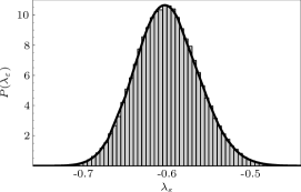
Figure 3: $\lambda_{\varepsilon}$-distribution for random Hermitian matrices from the GUE. The solid line shows the (normalized) probability density (6), the histogram is calculated form the eigenvectors of 400 different random matrices. $g=91$, $g^{\prime}=364$, $\Delta\lambda_{\varepsilon}^{2}=2/1425\approx 0.0014$, $\mathinner{\langle\hat{\sigma}_{z}\rangle}_{\text{can}}=-0.6$.

At first we assume that the two relevant bands in the environment are exactly degenerate and the transitions within S and C are exactly in resonance. In this case, $\hat{H}_{\text{S}}+\hat{H}_{\text{C}}\propto\hat{1}$ (within the relevant subspace spanned by the states (2)), thus we only need to deal with $\hat{H}_{\text{int}}$.

If the coupling $\hat{H}_{\text{int}}$ between system and environment is modeled by a random Hermitian matrix with a uniform Gaussian distribution $w(\hat{H}_{\text{int}})=C\exp(-A\operatorname{Tr}\{\hat{H}_{\text{int}}\}^{2})$ (i.e. taken from the GUE Haake (2001)), the state of the central system typically relaxes to the expected equilibrium state under Schrödinger dynamics for the total system Gemmer et al. (2004); Borowski et al. (2003); Schmidt and Mahler (2005). The state fluctuates in time, the amplitude of these fluctuations decreases with the size of the environment.

Figure 3 shows the $\lambda_{\varepsilon}$-distribution for these random Hermitian matrices. The histogram was obtained by choosing a number of random matrices with the given probability distribution and calculating the inversion of their eigenvectors. The parameters used are $g=91$ and $g^{\prime}=364$.

The probability density for the $\lambda_{\varepsilon}$’s for random Hermitian matrices from the GUE can be calculated analytically and is given by

$$P(\lambda)\propto(1-\lambda)^{g^{\prime}-1}(1+\lambda)^{g-1}.$$ (6)

This result is derived in appendix B. The solid line in figure 3 shows the distribution.

The mean value of $\lambda_{\varepsilon}$ for this distribution is given by

$$\bar{\lambda}_{\varepsilon}=\frac{g-g^{\prime}}{g+g^{\prime}}=\mathinner{\langle\hat{\sigma}_{z}\rangle}_{\text{can}},$$

as expected from the general result in appendix A. This is again the mean inversion of the equilibrium state for canonical relaxation.

The variance of this distribution is given by

$$\Delta\lambda_{\varepsilon}^{2}=4\frac{g\cdot g^{\prime}}{d^{2}(d+1)}$$

with $d=g+g^{\prime}$. Since this is finite, the reached steady state will typically deviate from the canonical equilibrium state.

For large systems, i.e. $d\rightarrow\infty$ (for constant ratio $g/g^{\prime}$), both $\Delta\lambda_{\varepsilon}^{2}$ and $\mathinner{\langle\bar{\sigma}_{z}\rangle}-\mathinner{\langle\hat{\sigma}_{z}\rangle}_{\text{can}}$ vanish. So in the thermodynamic limit, the quasi equilibrium reached equals canonical equilibrium.

IV.2 Random interaction

IV.2.1 Degenerate bands

We will now discuss a system that is not completely random, but has a random energy exchanging coupling between the central system and the environment. If the environmental bands are strictly degenerate, the Hamiltonian matrix has the form

$$\left(\begin{array}[]{@{}ccc|ccc@{}}-\varDelta/2&&&\\ &\ddots&&&\mathsf{V}^{\dagger}\\ &&-\varDelta/2\\ \hline\cr&&&\varDelta/2\\ &\mathsf{V}&&&\ddots\\ &&&&&\varDelta/2\end{array}\right),$$ (7)

where $\varDelta=\delta^{\text{S}}-\delta^{\text{C}}$ is the detuning between system and environment. The upper left block corresponds to the ground state of the central system, its therefore of dimension $g^{\prime}$, the lower right block (of dimension $g$) corresponds to the excited level. These blocks are purely diagonal.

The off diagonal block $\mathsf{V}$ (a $g\times{}g^{\prime}$ matrix), corresponding to energy exchange (canonical) coupling, is chosen randomly with normalized Gaussian distributions for the real and imaginary parts of the matrix elements.

For $\varDelta\neq 0$, system and environment are off resonance and the relaxation to the canonical equilibrium state is prohibited by energy conservation. So just $\varDelta=0$ is considered.

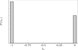
Figure 4: Random interaction, degenerate bands. The two bars represent delta-peaks of different strength. $\Delta\lambda_{\varepsilon}^{2}=6/25=0.24$.

Figure 4 shows the $\lambda_{\varepsilon}$-distribution for a matrix of type (7), again for $g=91$ and $g^{\prime}=364$. Instead of being single peaked, the distribution here is drastically different and consists of delta peaks at $\lambda_{\varepsilon}=-1$ and $\lambda_{\varepsilon}=0$, respectively. For a given Hamiltonian, there are exactly $g^{\prime}-g$ eigenstates with $\lambda_{\varepsilon}=-1$ and $2g$ eigenstates with $\lambda_{\varepsilon}=0$ (assuming $g^{\prime}>g$). The mean value still is $\bar{\lambda}_{\varepsilon}=(g-g^{\prime})/(g+g^{\prime})$, as expected.

However, the variance of the distribution is obviously considerably bigger. For the given parameters $\Delta\lambda_{\varepsilon}=0.24$ as opposed to $\Delta\lambda_{\varepsilon}\approx 0.0014$ for the completely random Hamiltonian. The deviation of the quasi equilibrium state for a Hamiltonian of type (7) from the canonical one is exactly

$$\mathinner{\langle\bar{\sigma}_{z}\rangle}-\mathinner{\langle\hat{\sigma}_{z}\rangle}_{\text{can}}=-\mathinner{\langle\hat{\sigma}_{z}\rangle}_{\text{can}}$$

which is nicely demonstrated in figure 5. Since this result is independent of the system size, going to large environments will not change the relaxation behavior other than reducing the amplitude of the fluctuations. Even in the thermodynamic limit the canonical equilibrium state is never reached.

Figure 5: Time evolution of the $z$-component of the Bloch vector of S for a random interaction and degenerate environmental bands, as described in section IV.2.1. Note that the canonical equilibrium state for the given parameters would be at $\mathinner{\langle\hat{\sigma}_{z}\rangle}=-0.6$.

IV.2.2 Non degenerate bands

Figure 6: A TLS in contact with an environment consisting of two “bands” with equidistant level spacing. Both bands have the same width $\delta\varepsilon$, the lower band consists of $g$ levels, the upper band of $g^{\prime}$ levels.

The situation, again, changes if we introduce a finite spacing between the levels within each environmental band. For simplicity we will only consider equidistant levels and equal bandwidth $\delta\varepsilon$ for both bands here. The lowest (and highest) levels of each band in the environment are in resonance with the central system. This system is depicted in figure 6 ($\delta_{\text{S}}=\delta_{\text{C}}$ is considered in the following). The Hamiltonian matrix in subspace (2) is given by.

$$\left(\begin{array}[]{@{}c|c@{}}\begin{array}[]{@{}cccc@{}}0\\ &\frac{\delta\varepsilon}{(g^{\prime}-1)}\\ &&\ddots\\ &&&\delta\varepsilon\end{array}&\mathsf{V}^{\dagger}\\ \hline\cr\mathsf{V}^{\dagger}&\begin{array}[]{@{}cccc@{}}0\\ &\frac{\delta\varepsilon}{(g-1)}\\ &&\ddots\\ &&&\delta\varepsilon\end{array}\end{array}\right)$$

By introducing a small level splitting in the environment (small compared to the interaction strength), the peaks in figure 4 get broader, especially the one at $\lambda_{\varepsilon}=0$ gets flatter considerably and is stretched towards negative $\lambda_{\varepsilon}$. The variance of the distribution gets smaller. Figure 7 shows the $\lambda_{\varepsilon}$-distribution for a relatively small level spacing.

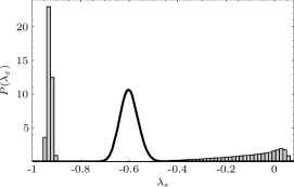
Figure 7: Random interaction, equidistant spacing, small level spacing. $\Delta\lambda_{\varepsilon}^{2}\approx 0.19$. The solid line shows the distribution for the complete random Hamiltonian.

When the level splitting is increased, the distributions becomes single peaked, with the peak close to its average and of similar height as the peak of the complete random Hamiltonian, see figure 8. A long tail towards higher $\lambda_{\varepsilon}$ prevails, therefore the variance is still considerably larger.

Figure 8: Random interaction, equidistant spacing, larger level spacing. The solid line shows the distribution for the complete random Hamiltonian. $\Delta\lambda_{\varepsilon}\approx 0.022$.

IV.3 Spin environments

We now consider a gapped spin or TLS as in figure 1 coupled to an array of spins, all with a Zeeman splitting equal to the central spin (or almost equal). Due to energy conservation, the system can be reduced to the situation shown in figure 1 for each pair of environmental bands. If the environment initially is in a canonical state, we can simply sum up over all bands, as long as the interaction between the environmental spins is small.

The $\lambda_{\varepsilon}$-distributions of several spin-environments have been discussed in Schmidt and Mahler (2005), so we will only discuss them briefly here.

IV.3.1 Spin-star configuration

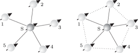
Figure 9: Schematics of the spin-star (left) and spin-ring (right) configurations. Typically, the environment consists of a lot more than five spins.

Figure 9 (left) shows schematically a spin-star configuration, i.e. a central spin coupled to an array of environmental spins without mutual interaction. A typical environment should of course consist of a lot more than 5 spins. The most general Hamiltonian describing the system-environment interaction is

$$\hat{H}_{\text{int}}=\sum_{i,j=1}^{3}\sum_{\nu=1}^{N}\gamma_{ij}^{(\nu)}\hat{\sigma}_{i}^{(\text{S})}\otimes\hat{\sigma}_{j}^{(\nu)}$$

for $N$ environmental spins.

It has been shown in Schmidt and Mahler (2005) that if the coefficients $\gamma_{ij}^{(\nu)}$ are chosen randomly, the initial state depicted in figure 4 typically does not relax to the canonical equilibrium state. The Hamiltonian matrix in this case has the form (7), however with small fluctuations on the diagonal, and the interaction part of the Hamiltonian matrix is only sparsely populated. Nevertheless, the $\lambda_{\varepsilon}$-distribution shows some similarity to the one described in section IV.2.2 for small level splitting. Figure 10 shows the $\lambda_{\varepsilon}$-distribution for this system.

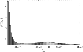
Figure 10: $\lambda_{\varepsilon}$-distribution for the spin-star configuration. 14 environmental spins, the 2nd and 3rd excited bands are considered, corresponding to $g=91$, $g^{\prime}=364$. $\Delta\lambda_{\varepsilon}^{2}\approx 0.216$.

IV.3.2 Intra-environmental coupling

If mutual coupling between the environmental spins is introduced, the situation changes. Figure 9 (right) schematically shows next neighbor coupling in the environment (spin-ring configuration), but other configurations are possible as well. As long as this coupling is weak, the system can still be considered band wise.

The interaction typically leads to a level splitting within the bands which in turn leads to a $\lambda_{\varepsilon}$-distribution similar to the one described in section IV.2.2 with bigger level splitting. Figure 11 shows the $\lambda_{\varepsilon}$-distribution for a spin-ring configuration. The shown distribution is for a $\hat{\sigma}_{x}\otimes\hat{\sigma}_{x}$ next neighbor coupling. The distributions for different kinds of coupling, e.g. Heisenberg coupling, are similar.

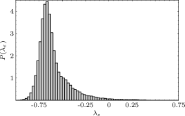
Figure 11: $\lambda_{\varepsilon}$-distribution for a spin-ring configuration. 14 environmental spins, the 2nd and 3rd excited bands are considered, corresponding to $g=91$, $g^{\prime}=364$. $\Delta\lambda_{\varepsilon}^{2}\approx 0.0295$.

IV.3.3 Inhomogeneous Zeeman splitting

If the individual environmental spins each have a different Zeeman splitting, the situation becomes similar to the one discussed in section IV.2.2. Figure 12 shows the $\lambda_{\varepsilon}$-distribution when the Zeeman splittings of the environmental spins are homogeneously distributed within a certain range. The distribution again shows a peak around the mean value $\bar{\lambda}_{\varepsilon}=\mathinner{\langle\hat{\sigma}_{z}\rangle}_{\text{can}}$, although broader than in the previous case.

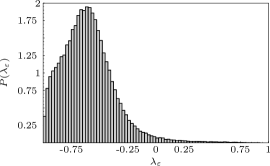
Figure 12: $\lambda_{\varepsilon}$-distribution for a spin-star configuration with inhomogeneous Zeeman splitting of the environmental spins. 14 environmental spins, the 2nd and 3rd excited bands are considered, corresponding to $g=91$, $g^{\prime}=364$. $\Delta\lambda_{\varepsilon}^{2}\approx 0.0548$.

V Width of the distribution and spectral width

Figures 4, 7, and 8 indicate that there is a continuous transition from a situation far from canonical to an almost canonical relaxation, depending on the environmental spectrum. What has been changed is the “strength” of the environmental spectrum from zero to the minimal variance of the $\lambda_{\varepsilon}$-distribution. A similar transition can be observed for many different environmental spectra.

In order to relate different types of spectra we split the Hamiltonian matrix (in the considered subspace) in its respective diagonal and off diagonal parts. The off diagonal part $\hat{H}_{\text{off}}$ ($\mathsf{V}$ and $\mathsf{V}^{\dagger}$ of (7)) describes the interaction between central system and environment, while the diagonal part $\hat{H}_{\text{diag}}$ describes the environmental spectra alone, if system and environment are in resonance. The diagonal part is always taken to be traceless. The quantity we use to compare different spectra is the relative strength of the environmental part to the interaction part,

$$V_{\text{R}}=\sqrt{\frac{\operatorname{Tr}(\hat{H}_{\text{diag}}^{2})}{\operatorname{Tr}(\hat{H}_{\text{off}}^{2})}.}$$

For a completely random matrix (GUE) this relation is given on average by

$$V_{\text{R,GUE}}=\sqrt{\frac{g^{2}+g^{\prime 2}}{2gg^{\prime}}}$$

which only depends on $g/g^{\prime}$, not on the actual size of the system.

Figure 13 shows the variance of the $\lambda_{\varepsilon}$-distribution for three different types of environmental spectra. In all three cases the environment consists of 14 spins, the 2nd and 3rd excited bands are considered, $g=91$, $g^{\prime}=364$, as described in section IV.3.

The solid line corresponds to the spin-ring configuration as described in section IV.3.2. The intra-environmental interaction is taken as a $\hat{\sigma}_{x}\otimes\hat{\sigma}_{x}+\hat{\sigma}_{y}\otimes\hat{\sigma}_{y}$ next neighbor coupling, the central system is randomly coupled to each environmental spin. The dashed line corresponds to the configuration described in section IV.3.3, there is no mutual interaction between the spins in the environment, but their Zeeman splitting is inhomogeneous. The central system is again coupled randomly to each environmental spin. The environmental spectrum for the dotted line is the same as for the dashed line. However, the interaction between the central spin and each environmental spin is modeled by $\hat{\sigma}_{x}\otimes\hat{\sigma}_{x}+\hat{\sigma}_{y}\otimes\hat{\sigma}_{y}$. The corresponding average values for a random matrix from the GUE are $\Delta\lambda_{\varepsilon}^{2}=2/1425\approx 0.0014$ and $V_{\text{R,GUE}}\approx 1.46$, respectively.

We notice that for each type of coupling and environmental spectrum there is a distinct minimum of $\Delta\lambda_{\varepsilon}^{2}$ for similar values of $V_{\text{R}}$ close to, but not exactly at the average value for the GUE matrices.

Figure 13: Variance of the $\lambda_{\varepsilon}$-distribution over the relative strength of the environmental spectrum for different types of this spectrum.

VI Conclusion

We have characterized situations under which non-thermal states should result as quasi-equilibrium states. For a spin-$1/2$ particle weakly coupled to a larger environment, there is a close relation between the quasi-equilibrium state of the small quantum system coupled to a larger environment and the distribution of certain properties of the energy eigenvectors of the total system. The equilibrium state is directly given by the width of this distribution. The spectral structure of the environment and the exact form of the coupling has a strong influence on the eigenvector distribution. To show this we have considered both abstract system Hamiltonians as well as Hamiltonians for structured spin environments.

Furthermore, there is a close relation between the width of the $\lambda_{\varepsilon}$-distribution and the strengths of both the local (diagonal) and the interaction (off diagonal) part of the Hamiltonian. By changing certain parameters within each system, there is a distinct minimum of the $\lambda_{\varepsilon}$-width for a value of the relative strength that’s close to the respective value for GUE matrices. This relative strength can thus give an indication whether for a given system relaxation to or close to a thermal state can be expected without calculating the full $\lambda_{\varepsilon}$-distribution. The relative width gives an indication how to choose the system parameters properly to achieve a certain type of equilibrium situation. This should be of help when designing a spin system for special (“non-thermal”) relaxation behavior.

We thank the Deutsche Forschungsgemeinschaft for financial support.

Appendix A Towards eq. (5)

Here we show that $\sum_{\varepsilon}\lambda_{\varepsilon}=g-g^{\prime}$.

$$\sum_{\varepsilon}\lambda_{\varepsilon} =\sum_{\varepsilon}\operatorname{Tr}_{\text{S}}\bigl{\{}\hat{\sigma}^{\text{S}}_{z}\operatorname{Tr}_{\text{C}}\mathinner{\lvert\varepsilon\rangle}\!\mathinner{\langle\varepsilon\rvert}\bigr{\}}$$

$$=\sum_{\varepsilon}\operatorname{Tr}\bigl{\{}(\hat{\sigma}^{\text{S}}_{z}\otimes\hat{1}^{\text{C}})\mathinner{\lvert\varepsilon\rangle}\!\mathinner{\langle\varepsilon\rvert}\bigr{\}}=\operatorname{Tr}\bigl{\{}(\hat{\sigma}^{\text{S}}_{z}\otimes\hat{1}^{\text{C}})\bigr{\}},$$

the last equality follows from the fact that the energy eigenvectors are a complete orthonormal basis in Hilbert space. If we now use the basis $\{\mathinner{\lvert 0,m^{\prime}\rangle},\mathinner{\lvert 1,m\rangle}\}$ to calculate the trace ($m$ and $m^{\prime}$ denote the levels in band $k$ and $k^{\prime}$, respectively), we see that the $g$ kets $\mathinner{\lvert 1,m\rangle}$ yield $1$’s, while the $g^{\prime}$ kets $\mathinner{\lvert 0,m^{\prime}\rangle}$ yield $-1$’s and the total trace equals $g-g^{\prime}$.

Appendix B Derivation of eq. (6)

If we introduce the basis $\{\mathinner{\lvert k{:}m\rangle}\}$ ($1<m\leq g_{k}$) for the band $k$ and the basis $\{\mathinner{\lvert k^{\prime}{:}m\rangle}\}$ for the band $k^{\prime}$, we can write the state of the total system as ($g=g_{k}$, $g^{\prime}=g_{k^{\prime}}$)

$$\mathinner{\lvert\psi\rangle}=\sum_{m=1}^{g^{\prime}}\psi_{0m}\mathinner{\lvert 0\rangle}\otimes\mathinner{\lvert k^{\prime}{:}m\rangle}+\sum_{m=1}^{g}\psi_{1m}\mathinner{\lvert 1\rangle}\otimes\mathinner{\lvert k{:}m\rangle}\!.$$

The reduced state of the central system becomes

$$\hat{\rho}_{\text{S}}=\operatorname{Tr}_{\text{C}}\hat{\rho}=\sum_{m=1}^{g^{\prime}}\lvert\psi_{0m}\rvert^{2}\mathinner{\lvert 0\rangle}\!\mathinner{\langle 0\rvert}+\sum_{m=1}^{g}\lvert\psi_{1m}\rvert^{2}\mathinner{\lvert 1\rangle}\!\mathinner{\langle 1\rvert}.$$

We are interested in the distribution of the inversion of the energy eigenstates of certain Hamiltonians. Since the inversion is determined by the population of each level, we will derive the distribution for the population of the ground state, $p_{0}=\sum_{m}\lvert\psi_{0m}\rvert^{2}$.

For simplicity we introduce a single index $n$ to label the amplitudes instead of the double index $0m$ or $1m$. $n$ runs from $1$ to $d=g+g^{\prime}$ (the reduced Hilbert space dimension). In this notation $p_{0}=\sum_{n=1}^{g^{\prime}}\lvert\psi_{n}\rvert^{2}$.

We now split the amplitudes into real and imaginary part, $\psi_{n}=x_{k}+\mathrm{i}{}x_{k+1}$, where $1\leq{}k\leq{}2g^{\prime}$ corresponds to $\mathinner{\lvert 0\rangle}\!\mathinner{\langle 0\rvert}$ and $2g^{\prime}+1\leq{}k\leq{}2d$ corresponds to $\mathinner{\lvert 1\rangle}\!\mathinner{\langle 1\rvert}$, therefore $p_{0}=\sum_{k=1}^{2g^{\prime}}x_{k}$. The combined probability density of the first $2g^{\prime}$ amplitudes $x_{k}$ for eigenvectors of random matrices from the GUE is given by Haake (2001)

$$P_{\text{a}}(x_{1},\ldots,x_{2g^{\prime}})=\pi^{-1/2}\frac{\varGamma(d)}{\varGamma(d-g^{\prime})}\biggl{(}1-\sum_{k=1}^{2g^{\prime}}x_{k}^{2}\biggr{)}^{d-g^{\prime}-1}.$$

The desired probability density for the population of the ground state $p_{0}$ is given by

$$P_{\text{p}}(p_{0})=\int\mathrm{d}^{2g^{\prime}}\!x\,P_{\text{a}}(x_{1},\ldots,x_{2g^{\prime}})\,\delta\biggl{(}p_{0}-\sum_{k=1}^{2g^{\prime}}x_{k}^{2}\biggr{)},$$

integrating over the unit sphere in $2g^{\prime}$-dimensional space. The integral yields

$$P_{\text{p}}(p_{0})=\frac{\varGamma(d)}{\varGamma(d-g^{\prime})\varGamma(g^{\prime})}\,p_{0}^{g^{\prime}-1}(1-p_{0})^{d-g^{\prime}-1}.$$

Transforming to $\lambda=1-2p_{0}$ finally gives the probability density (6),

$$P(\lambda)=\frac{1}{2^{d-1}}\frac{\varGamma(d)}{\varGamma(d-g^{\prime})\varGamma(g^{\prime})}(1-\lambda)^{g^{\prime}-1}(1+\lambda)^{d-g^{\prime}-1}.$$ (6’)

References

- Gemmer et al. (2004) J. Gemmer, M. Michel, and G. Mahler, Quantum Thermodynamics: The Emergence of Thermodynamical Behaviour within Composite Quantum Systems (Springer, Berlin, 2004).
- Borowski et al. (2003) P. Borowski, J. Gemmer, and G. Mahler, Eur. Phys. J. B 35, 255 (2003).
- Briegel and Raussendorf (2001) H. J. Briegel and R. Raussendorf, Phys. Rev. Lett. 86, 910 (2001).
- O’Connor and Wootters (2001) K. M. O’Connor and W. K. Wootters, Phys. Rev. A 63, 052302 (2001).
- Wang (2002) X. Wang, Phys. Rev. A 66, 034302 (2002).
- Hutton and Bose (2004a) A. Hutton and S. Bose, Phys. Rev. A 69, 042312 (2004a).
- Hutton and Bose (2004b) A. Hutton and S. Bose, quant-ph/0408077 (2004b).
- Vidal et al. (2003) G. Vidal, J. I. Latorre, E. Rico, and A. Kitaev, Phys. Rev. Lett. 90, 227902 (2003).
- Breuer et al. (2004) H.-P. Breuer, D. Burgarth, and F. Petruccione, Phys. Rev. B 70, 045323 (2004).
- Lages et al. (2004) J. Lages, V. V. Dobrovitski, and B. N. Harmon, quant-ph/0406001 (2004).
- Imamoḡlu et al. (1999) A. Imamoḡlu, D. D. Awschalom, G. Burkard, D. P. DiVincenzo, D. Loss, M. Sherwin, and A. Small, Phys. Rev. Lett. 83, 4204 (1999).
- Makhlin et al. (1999) Y. Makhlin, G. Schön, and A. Shnirman, Nature 398, 305 (1999).
- Schmidt and Mahler (2005) H. Schmidt and G. Mahler, Phys. Rev. E 72, 016117 (2005).
- Haake (2001) F. Haake, Quantum Signatures of Chaos (Springer, Berlin, 2001).