Joint Entropy of the Harmonic Oscillator with Time Dependent Mass and Frequency

Abstract

Time dependent entropy of harmonic oscillator with time dependent mass and frequency are investigated. The joint entropy so called Leipnik’s entropy is calculated by using time dependent wave function obtained by the Feynman path integral method. It is shown that, Leipnik’s entropy fluctuates with time. However in constant mass and time dependent frequency case, entropy increases monotonically with time.

Keywords: Path integral, joint entropy, harmonic oscillator with time dependent mass and frequency.

I Introduction

The information entropy plays a major role in a stronger formulation of the uncertainty relations ekrem . This relation may be mathematically defined by using the Boltzmann-Shannon information entropy and the von Neumann entropy. For both open and closed quantum systems, different information-theoretical entropy measures have been discussed Zurek ; Omnes ; Anastopoulos . The joint entropy Leipnik ; Dodonov can also be used to explain the properties of the loss of information evolving pure quantum states Trigger . The joint entropy of the physical systems were conjectured by Dunkel and Trigger Dunkel in which their systems named MACS (maximal classical states). The Leipnik entropy of the simple harmonic oscillator was determined not monotonically increase with time Garbaczewski . In this work, we give a uniform description of the complete joint entropy information for time dependent entropy of harmonic oscillator with time dependent mass and frequency. The study of harmonic oscillators with time dependent frequencies or with time dependent masses (or both simultaneously) has attracted considerable interest in past few years but the investigation of joint entropy of this system have not been studied yet. The time-dependent harmonic oscillator has invoked much attention because of its many applications in different areas of physics, such as quantum optics and plasma physics Dandas ; Abdalla ; Lemos ; Ben .

This paper is organized as follows. In section II, we explain fundamental definitions needed for the calculation. In section III, we get the results for harmonic oscillator with time dependent mass and frequency. Moreover, we obtain the analytical solution of kernel and using this, wave function in both coordinate and momentum space and its joint entropy were calculated. In this section, we also investigated same quantities for harmonic oscillator with strongly pulsating mass and inverse square time dependent frequency. Finally, we present the conclusion in section IV.

II Fundamental Definitions

We consider a classical system with $d=sN$ degrees of freedom, where N is the particle number and s is number of spatial dimensions Dunkel . The density function $g(x,p,t)=g(x_{1},...,x_{d},p_{1},...,p_{d},t)$ which is non-negative, time dependent phase space density function of the system is assuming to be normalized to unity,

$$\int dxdpg(x,p,t)=1.$$ (1)

The Gibbs-Shannon entropy is described by

$$S(t)=-\frac{1}{N!}\int dxdpg(x,p,t)ln(h^{d}g(x,p,t)),$$ (2)

where $h=2\pi\hbar$ is the Planck constant. Schrödinger wave equation with the Born interpretation Born is given by

$$i\hbar\frac{\partial\psi}{\partial t}=\hat{H}\psi.$$ (3)

The quantum probability densities are defined in position and momentum spaces as $|\psi(x,t)|^{2}$ and $|\tilde{\psi}(p,t)|^{2}$, where $|\tilde{\psi}(p,t)|^{2}$ is given as

$$\tilde{\psi}(p,t)=\int\frac{dxe^{-ipx/\hbar}}{(2\pi\hbar)^{d/2}}\psi(x,t).$$ (4)

Leipnik proposed the product function as Dunkel .

$$g_{j}(x,p,t)=|\psi(x,t)|^{2}|\tilde{\psi}(p,t)|^{2}\geq 0.$$ (5)

Substituting Eq. (5) into Eq. (2), we get the joint entropy $S_{j}(t)$ for the pure state $\psi(x,t)$ or equivalently it can be written in the following form  Dunkel

$$S_{j}(t) = -\int dx|\psi(x,t)|^{2}\ln|\psi(x,t)|^{2}-\int dp|\tilde{\psi}(p,t)|^{2}\ln|\tilde{\psi}(p,t)|^{2}-$$ (6)

$$- \ln h^{d}.$$

We find time dependent wave function by means of the Feynman path integral which has form Feynman

$$K(x^{\prime\prime},t^{\prime\prime};x^{\prime},t^{\prime}) = \int^{x^{\prime\prime}=x(t^{\prime\prime})}_{x^{\prime}=x(t^{\prime})}Dx(t)e^{\frac{i}{\hbar}S[x(t)]}$$ (7)

$$= \int^{x^{\prime\prime}}_{x^{\prime}}Dx(t)e^{\frac{i}{\hbar}\int_{t^{\prime}}^{t^{\prime\prime}}L[x,\dot{x},t]dt}.$$

The Feynman kernel can be related to the time dependent Schrödinger’s wave function

$$K(x^{\prime\prime},t^{\prime\prime};x^{\prime},t^{\prime})=\sum_{n=0}^{\infty}\psi_{n}^{*}(x^{\prime},t^{\prime})\psi_{n}(x^{\prime\prime},t^{\prime\prime}).$$ (8)

The propagator in semiclassical approximation reads

$$K(x^{\prime\prime},t^{\prime\prime};x^{\prime},t^{\prime})=\Big{[}\frac{i}{2\pi\hbar}\frac{\partial^{2}}{\partial x^{\prime}\partial x^{\prime\prime}}S_{cl}(x^{\prime\prime},t^{\prime\prime};x^{\prime},t^{\prime})\Big{]}^{1/2}e^{\frac{i}{\hbar}S_{cl}(x^{\prime\prime},t^{\prime\prime};x^{\prime},t^{\prime})}.$$ (9)

The prefactor is often referred to as the Van Vleck-Pauli-Morette determinant  Khandekar ; Kleinert . The $F(x^{\prime\prime},t^{\prime\prime};x^{\prime},t^{\prime})$ is given by

$$F(x^{\prime\prime},t^{\prime\prime};x^{\prime},t^{\prime})=\Big{[}\frac{i}{2\pi\hbar}\frac{\partial^{2}}{\partial x^{\prime}\partial x^{\prime\prime}}S_{cl}(x^{\prime\prime},t^{\prime\prime};x^{\prime},t^{\prime})\Big{]}^{1/2}.$$ (10)

III Harmonic Oscillator with Time Dependent Mass and Frequency

The Lagrangian of the harmonic oscillator with time-dependent frequency and mass are given by

$$L=\frac{1}{2}m(t)\dot{x}^{2}-\frac{1}{2}m(t)\omega^{2}(t)x^{2},$$ (11)

where $\omega(t)$ and $m(t)$ are, respectively, the frequency and mass associated with oscillator, and which are arbitrary real functions of time. The classical equation of motion for the Lagrangian is

$$\ddot{x}+2\frac{\dot{\eta}}{\eta}\dot{x}+\omega^{2}(t)x=0,$$ (12)

where $\eta(t)=\sqrt{m}$. The solution to the equation of motion is given by

$$x(t)=\frac{\alpha(t)}{\eta(t)}\Big{[}A\cos\gamma(t)+B\sin\gamma(t)\Big{]},$$ (13)

where $\frac{\alpha(t)}{\eta(t)}=\rho(t)$, $\gamma(t)$ refers to the amplitude and phase of classical oscillators and A and B are constants. The function $\rho(t)$ have to satisfy the following equation:

$$\ddot{\rho}+\frac{\dot{m}}{m}\dot{\rho}+\omega^{2}(t)\rho(t)=\frac{1}{m^{2}\rho^{3}}.$$ (14)

The constant A and B in Eq.(13) can be determined by using the boundary conditions of $x(t^{\prime})=x^{\prime}$ and $x(t^{\prime\prime})=x^{\prime\prime}$. The A and B coefficients yield as

$$A=\frac{1}{\sin(\gamma^{\prime\prime}-\gamma^{\prime})}\Big{(}\frac{x^{\prime}}{\rho^{\prime}}\sin\gamma^{\prime\prime}-\frac{x^{\prime\prime}}{\rho^{\prime\prime}}\sin\gamma^{\prime}\Big{)},$$ (15)

and

$$B=\frac{1}{\sin(\gamma^{\prime\prime}-\gamma^{\prime})}\Big{(}\frac{x^{\prime\prime}}{\rho^{\prime\prime}}\cos\gamma^{\prime}-\frac{x^{\prime}}{\rho^{\prime}}\cos\gamma^{\prime\prime}\Big{)}.$$ (16)

Substituting A and B into Eq.(13), the classical path that connects the point of $(x^{\prime},t^{\prime})$ and $(x^{\prime\prime},t^{\prime\prime})$ can be written as

$$x_{cl}=\frac{\rho}{\sin(\gamma^{\prime\prime}-\gamma^{\prime})}\Big{(}\frac{x^{\prime}}{\rho^{\prime}}\sin(\gamma^{\prime\prime}-\gamma)-\frac{x^{\prime\prime}}{\rho^{\prime\prime}}\sin(\gamma^{\prime\prime}-\gamma)\Big{)}.$$ (17)

Substituting the classical paths into action function, the classical action becomes

$$S_{cl} = \frac{m^{\prime\prime}x^{\prime\prime 2}}{2}\Big{(}\frac{\dot{\rho}^{\prime\prime}}{\rho^{\prime\prime}}\Big{)}-\frac{m^{\prime}x^{\prime 2}}{2}\Big{(}\frac{\dot{\rho}^{\prime}}{\rho^{\prime}}\Big{)}+\frac{1}{2}\Big{(}\frac{x^{\prime\prime 2}}{\rho^{\prime\prime 2}}+\frac{x^{\prime\prime 2}}{\rho^{\prime\prime 2}}\Big{)}\cot(\gamma^{\prime\prime}-\gamma^{\prime})-$$ (18)

$$- \frac{x^{\prime\prime}x^{\prime}}{\rho^{\prime\prime}\rho^{\prime}}\csc(\gamma^{\prime\prime}-\gamma^{\prime}).$$

By substituting the above action into Eq.(10), the factor can be obtained as

$$F(x^{\prime\prime},t^{\prime\prime};x^{\prime},t^{\prime})=\Big{[}\frac{1}{2i\pi\hbar\rho^{\prime}\rho^{\prime\prime}\sin(\gamma^{\prime\prime}-\gamma^{\prime})}\Big{]}^{1/2}.$$ (19)

Therefore the propagator for the harmonic oscillator with a time dependent mass and frequency can be obtained by

$$K(x^{\prime\prime},t^{\prime\prime};x^{\prime},t^{\prime}) = \Big{[}\frac{1}{2i\pi\hbar\rho^{\prime}\rho^{\prime\prime}\sin(\gamma^{\prime\prime}-\gamma^{\prime})}\Big{]}^{1/2}\exp\Big{[}\frac{i}{2\hbar}\Big{[}\frac{m^{\prime\prime}x^{\prime\prime 2}}{2}\Big{(}\frac{\dot{\rho}^{\prime\prime}}{\rho^{\prime\prime}}\Big{)}-$$ (20)

$$- \frac{m^{\prime}x^{\prime 2}}{2}\Big{(}\frac{\dot{\rho}^{\prime}}{\rho^{\prime}}\Big{)}\Big{]}\Big{]}\exp\Big{[}\frac{i}{2\hbar\sin(\gamma^{\prime\prime}-\gamma^{\prime})}\Big{(}\frac{x^{\prime\prime 2}}{\rho^{\prime\prime 2}}+\frac{x^{\prime 2}}{\rho^{\prime 2}}\Big{)}\times$$

$$\times \cos(\gamma^{\prime\prime}-\gamma^{\prime})-\frac{2x^{\prime\prime}x^{\prime}}{\rho^{\prime}\rho^{\prime\prime}}\Big{]}.$$

By the use of the Mehler-formula

$$e^{-(x^{2}+y^{2})/2}\sum_{n=0}^{\infty}\frac{1}{n!}(\frac{z}{2})^{2}H_{n}(x)H_{n}(y) = \frac{1}{\sqrt{1-z^{2}}}\exp[\frac{4xyz}{2(1-z^{2})}-$$ (21)

$$- \frac{(x^{2}+y^{2})(1+z^{2})}{2(1-z^{2})}],$$

where $H_{n}$ is Hermite polynomials, we can write the Feynman kernel in form

$$K(x^{\prime\prime},t^{\prime\prime};x^{\prime},t^{\prime}) = \frac{1}{2^{n}n!}\Big{[}\frac{1}{2i\pi\hbar\rho^{\prime}\rho^{\prime\prime}\sin(\gamma^{\prime\prime}-\gamma^{\prime})}\Big{]}^{1/2}\exp\Big{[}\frac{i}{2\hbar}\Big{[}\frac{m^{\prime\prime}x^{\prime\prime 2}}{2}\Big{(}\frac{\dot{\rho}^{\prime\prime}}{\rho^{\prime\prime}}\Big{)}-$$ (22)

$$- \frac{m^{\prime}x^{\prime 2}}{2}\Big{(}\frac{\dot{\rho}^{\prime}}{\rho^{\prime}}\Big{)}\Big{]}\Big{]}\exp\Big{[}-\frac{1}{2\hbar}\Big{(}\frac{x^{\prime\prime 2}}{\rho^{\prime\prime 2}}+\frac{x^{\prime 2}}{\rho^{\prime 2}}\Big{)}\Big{]}\sum H_{n}\Big{[}\sqrt{\frac{1}{\hbar}}\frac{x^{\prime\prime}}{\rho^{\prime\prime}}\Big{]}\times$$

$$\times H_{n}\Big{[}\sqrt{\frac{1}{\hbar}}\frac{x^{\prime}}{\rho^{\prime}}\Big{]}\exp\Big{(}-i\gamma(n+\frac{1}{2})\Big{)}.$$

Comparing the kernel in Eq. (22) with Eq. (8), the wave function for harmonic oscillator with time dependent mass and frequency can be found as

$$\Psi_{n}(x,t) = \exp[i\alpha_{n}(t)]\Big{[}\frac{1}{\pi^{1/2}\hbar^{1/2}n!2^{n}\rho}\Big{]}^{1/2}\exp\Big{[}\frac{im(t)}{2\hbar}\Big{(}\frac{\dot{\rho}}{\rho}+\frac{i}{m(t)\rho^{2}}\Big{)}x^{2}\Big{]}\times$$ (23)

$$\times H_{n}\Big{[}\Big{(}\frac{1}{\hbar}\Big{)}^{1/2}\frac{x}{\rho}\Big{]},$$

where the phase functions $\alpha_{n}(t)$ are described by

$$\alpha_{n}(t)=-\Big{(}n+\frac{1}{2}\Big{)}\int_{0}^{t}\frac{1}{m(t^{\prime})\rho^{2}}dt^{\prime}.$$ (24)

This result is also briefly obtained before by using the Feynman Path Integral method in Ref.Khandekar . It is also in agreement with ones obtained in Refs.  Pedrosa and  Ciftja . The time dependent wave function of ground state is

$$\Psi_{0}(x,t) = \exp[i\alpha_{0}(t)]\Big{[}\frac{1}{\pi^{1/2}\hbar^{1/2}\rho}\Big{]}^{1/2}\exp\Big{[}\frac{im(t)}{2\hbar}\Big{(}\frac{\dot{\rho}}{\rho}+\frac{i}{m(t)\rho^{2}}\Big{)}x^{2}\Big{]}.$$ (25)

Note that when $m(t)\rightarrow m$, $\omega(t)\rightarrow\omega_{0}$ and $\rho(t)\rightarrow\rho_{0}=const=1/\sqrt{m\omega_{0}}$, the solution in Eq.(23) becomes the solution for the time independent harmonic oscillator of mass m and frequency $\omega_{0}$.

III.1 Time dependent mass and constant frequency

In this calculation, we choose harmonic oscillator constant frequency and time dependent mass which is called pulsating mass. For instance, it has been shown that the Lagrangian describing the problem of a Fabry-Perot cavity in contact with a heat reservoir assumes the form of constant frequency and time dependent mass Colegrave . The time dependence of the mass can be taken as $m(t)=m\cos^{2}(\nu t)$ where $\nu$ is described as frequency of pulsating mass. The Lagrangian of the system is

$$L=\frac{1}{2}m\cos^{2}(\nu t)\dot{x}^{2}-\frac{1}{2}m\cos^{2}(\nu t)\omega^{2}x^{2}.$$ (26)

The kernel for a harmonic oscillator with strongly pulsating mass can be obtained from Eq. (20) as

$$K(x^{\prime\prime},t^{\prime\prime};x^{\prime},t^{\prime}) = \Big{[}\frac{m\Omega\cos\nu t^{\prime}\cos\nu t^{\prime\prime}}{2i\pi\hbar\sin\Omega(t^{\prime\prime}-t^{\prime})}\Big{]}^{1/2}\exp\Big{[}\frac{im\nu}{2\hbar}\Big{(}\cos^{2}\nu\tan\nu t^{\prime\prime}x^{\prime\prime 2}-$$ (27)

$$- \cos^{2}\nu t^{\prime}\tan\nu t^{\prime}x^{\prime 2}\Big{)}\Big{]}\exp\Big{[}\frac{im\Omega}{2\hbar\sin(\Omega t^{\prime\prime}-t^{\prime})}\Big{(}\cos^{2}\nu t^{\prime\prime}x^{\prime\prime 2}+$$

$$+ \cos^{2}\nu t^{\prime}x^{\prime 2}\Big{)}\cos\Omega(t^{\prime\prime}-t^{\prime})-2\cos\nu t^{\prime}\cos\nu t^{\prime\prime}x^{\prime\prime}x^{\prime}\Big{]},$$

where we use $\Omega^{2}=\omega^{2}+\nu^{2}$. Using Eq. (21) Mehler formula, and then the time dependent wave function was obtained as

$$\Psi_{n}(x,t) = \exp[-i\beta_{n}(t)]\Big{[}\frac{m(t)\Omega}{\pi\hbar n!^{2}2^{2n}}\Big{]}^{1/4}\exp\Big{[}\frac{im(t)}{2\hbar}\Big{(}\nu\tan\nu t+i\Omega\Big{)}x^{2}\Big{]}\times$$ (28)

$$\times H_{n}\Big{[}\Big{(}\frac{m(t)\Omega}{\hbar}\Big{)}^{1/2}x\Big{]},$$

where the phase functions $\beta_{n}(t)$ is described as

$$\beta_{n}(t)=(n+1/2)\Omega t.$$ (29)

Note that when $\nu\rightarrow 0$ and $m(t)\rightarrow m=const$, the solution in Eq.(28) reduces to the solution for the time independent harmonic oscillator of mass m and frequency $\omega_{0}$. The ground state wave function yields as

$$\Psi_{0}(x,t) = \exp[-i(1/2)\Omega t]\Big{[}\frac{m(t)\Omega}{\pi\hbar}\Big{]}^{1/4}\exp\Big{[}\frac{im(t)}{2\hbar}\Big{(}\nu\tan\nu t+i\Omega\Big{)}x^{2}\Big{]}.$$ (30)

The density of probability in coordinate space is

$$|\Psi_{0}(x,t)|^{2} = \Big{[}\frac{m(t)\Omega}{\pi\hbar}\Big{]}^{1/2}\exp\Big{[}-\frac{m(t)\Omega}{\hbar}x^{2}\Big{]}.$$ (31)

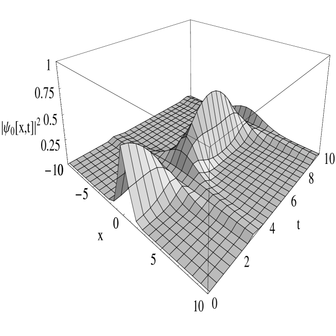
Figure 1: $|\Psi_{0}(x,t)|^{2}$ versus time and coordinate for strongly pulsating mass and constant frequency.

In Fig.1, the density of probability in coordinate space is shown. The density of probability in momentum space can be easily calculated as

$$|\Psi_{0}(p,t)|^{2} = \Big{[}\frac{\Omega}{\hbar\pi m(\nu^{2}\tan^{2}\nu t+\Omega^{2})}\Big{]}^{1/2}\exp\Big{[}-\frac{p^{2}\Omega}{m\hbar(\nu^{2}\tan^{2}\nu t+\Omega^{2})}\Big{]}.$$ (32)

The joint entropy for ground state from Eq. (6) becomes

$$S_{j}(t) = \frac{1}{2}\Big{[}\ln\Big{(}\frac{e^{2}}{4}\Big{)}+\ln\Big{(}\frac{1}{\pi\hbar\sqrt{m(t)\Omega}}\Big{)}$$ (33)

$$+ \sqrt{m(t)\Omega}\Big{(}1-\ln\frac{\Omega}{\pi\hbar(\nu^{2}\tan^{2}\nu t+\Omega^{2})}\Big{)}\Big{]}.$$

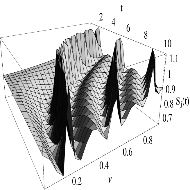
Figure 2: The 3D graph of joint entropy of harmonic oscillator with time dependent mass and constant frequency.

The joint entropy of harmonic oscillator with time dependent mass and constant frequency is plotted in Fig.2. The small $\nu$ and large $\nu$ cases are shown in Fig.3 and Fig.4, respectively.

III.2 Time dependent frequency and constant mass

The Lagrangian of the harmonic oscillator with time-dependent frequency is given by

$$L=\frac{1}{2}m\dot{x}^{2}-\frac{1}{2}m\omega(t)^{2}x^{2}.$$ (34)

The time dependent frequency is described by

$$\omega(t)=\frac{\omega_{0}}{t^{2}}.$$ (35)

In this case, we defined the following quantities

$$\rho(t)=\frac{1}{\sqrt{m\omega(t)}},$$ (36)

and

$$\gamma(t)=-\frac{\omega_{0}}{t}.$$ (37)

By substituting Eqs. (35), (36) and (37) into the general kernel Eq. (20), the kernel for a harmonic oscillator with the inverse square time dependent frequency can be derived as

$$K(x^{\prime\prime},t^{\prime\prime};x^{\prime},t^{\prime}) = \Big{[}\frac{m\omega_{0}}{2i\pi\hbar t^{\prime}t^{\prime\prime}\sin\omega_{0}\Big{(}\frac{t^{\prime\prime}-t^{\prime}}{t^{\prime}t^{\prime\prime}}\Big{)}}\Big{]}^{1/2}\exp\Big{[}\frac{i}{2\hbar}\Big{(}\frac{mx^{\prime\prime 2}}{t^{\prime\prime}}-\frac{mx^{\prime 2}}{t^{\prime}}\Big{)}\Big{]}\times$$ (38)

$$\times \exp\Big{[}\frac{im\omega_{0}}{2\hbar\sin\omega_{0}\Big{(}\frac{t^{\prime\prime}-t^{\prime}}{t^{\prime}t^{\prime\prime}}\Big{)}}\Big{[}\Big{(}\frac{x^{\prime\prime 2}}{t^{\prime\prime 2}}+\frac{x^{\prime 2}}{t^{\prime 2}}\Big{)}\cos\omega_{0}\Big{(}\frac{t^{\prime\prime}-t^{\prime}}{t^{\prime}t^{\prime\prime}}\Big{)}-\frac{2x^{\prime}x^{\prime\prime}}{t^{\prime}t^{\prime\prime}}\Big{]}.$$

Using Eq. (21) Mehler formula, we obtain the kernel

$$K(x^{\prime\prime},t^{\prime\prime};x^{\prime},t^{\prime}) = \Big{[}\frac{m\omega_{0}}{\pi\hbar t^{\prime}t^{\prime\prime}}\Big{]}^{1/2}\exp\Big{[}\frac{i}{2\hbar}\Big{(}\frac{mx^{\prime\prime 2}}{t^{\prime\prime}}-\frac{mx^{\prime 2}}{t^{\prime}}\Big{)}\Big{]}\times$$ (39)

$$\times \exp\Big{[}-\frac{m\omega_{0}}{2\hbar}\Big{[}\Big{(}\frac{x^{\prime\prime 2}}{t^{\prime\prime 2}}+\frac{x^{\prime 2}}{t^{\prime 2}}\Big{)}\Big{]}\sum_{0}^{\infty}H_{n}\Big{(}\sqrt{\frac{m\omega_{0}}{\hbar}}\frac{x^{\prime\prime}}{t^{\prime\prime}}\Big{)}H_{n}\Big{(}\sqrt{\frac{m\omega_{0}}{\hbar}}\frac{x^{\prime}}{t^{\prime}}\Big{)}\times$$

$$\times \frac{\exp(\frac{i\omega_{0}}{t}(n+1/2))}{2^{n}n!}.$$

Using the Eq. (8), the time dependent wave function was derived as

$$\Psi_{n}(x,t) = \frac{1}{\sqrt{2^{n}n!t}}\Big{[}\frac{m\omega_{0}}{\pi\hbar}\Big{]}^{1/4}\exp\Big{(}\Big{(}n+\frac{1}{2}\Big{)}\frac{i\omega_{0}}{t}\Big{)}\exp\Big{[}\frac{im}{2\hbar t}\Big{(}1+\frac{i\omega_{0}}{t}\Big{)}x^{2}\Big{]}\times$$ (40)

$$\times H_{n}\Big{(}\sqrt{\frac{m\omega_{0}}{\hbar}}\frac{x}{t}\Big{)}.$$

The time dependent wave function for ground state is given by

$$\Psi_{0}(x,t) = \Big{[}\frac{m\omega_{0}}{\pi\hbar t^{2}}\Big{]}^{1/4}\exp\Big{(}\frac{i\omega_{0}}{2t}\Big{)}\exp\Big{[}\frac{im}{2\hbar t}\Big{(}1+\frac{i\omega_{0}}{t}\Big{)}x^{2}\Big{]}.$$ (41)

The density of probability in coordinate space is

$$|\Psi_{0}(x,t)|^{2} = \Big{[}\frac{m\omega_{0}}{\pi\hbar t^{2}}\Big{]}^{1/2}\exp\Big{[}-\frac{m\omega_{0}}{\hbar t^{2}}x^{2}\Big{]}.$$ (42)

The density of probability for coordinate space is shown in Fig.5. The density of probability in momentum space can be easily calculated as

$$|\Psi_{0}(p,t)|^{2} = \Big{[}\frac{\omega_{0}t^{2}}{(\omega_{0}^{2}+t^{2})\hbar\pi m}\Big{]}^{1/2}\exp\Big{[}-\frac{p^{2}\omega_{0}t^{2}}{m\hbar(\omega_{0}^{2}+t^{2})}\Big{]}.$$ (43)

Note that when $t\rightarrow 1$ and $\omega(t)\rightarrow\omega_{0}=const$, the solution of Eqs.(42) and (43) become the solution for the time independent harmonic oscillator of mass m and frequency $\omega_{0}$. The joint entropy for ground state from Eq. (6) becomes

$$S_{j}(t)=\ln\Big{[}\Big{(}\frac{e}{2}\Big{)}\Big{(}\frac{\omega_{0}^{2}+t^{2}}{\omega_{0}^{2}}\Big{)}^{1/2}\Big{]}.$$ (44)

The contour and joint entropy of harmonic oscillator with inverse square time dependent frequency are shown in Figs. 6 and 7, respectively. It is important that Eq. (44) is in agreement with following general inequality for the joint entropy:

$$S_{j}(t)\geq\ln(\frac{e}{2}).$$ (45)

originally derived by Leipnik for arbitrary one-dimensional one-particle wave functionsLeipnik ; Dunkel .

IV Conclusion

We have investigated the joint entropy for explicit time dependent solution of one-dimensional harmonic oscillators with time dependent frequency and mass. The time dependent wave function is obtained by means of Feynman Path integral technique. In the time dependent strongly pulsating mass, harmonic oscillator with constant frequency case, we have found that the joint entropy fluctuated with time and frequency. It is seen that, the joint entropy has harmonic behavior. This result indicates that the information periodically transfers between harmonic oscillators with strongly pulsating masses. On the other hand, inverse square time frequency case, the joint entropy of harmonic oscillator with time dependent frequency shows remarkable monotonically increase with time. In the $\omega(t)\rightarrow\omega=constant$ and $\nu\rightarrow 0$, case theses results agree with time independent harmonic oscillator. It also depends on choice of initial frequency as seen in Fig. 7.

V Acknowledgements

This research was partially supported by the Scientific and Technological Research Council of Turkey.

Figure 3: The joint entropy of harmonic oscillator with time dependent mass and constant frequency versus small $\nu$.

Figure 4: The joint entropy of harmonic oscillator with time dependent mass and constant frequency versus large $\nu$.

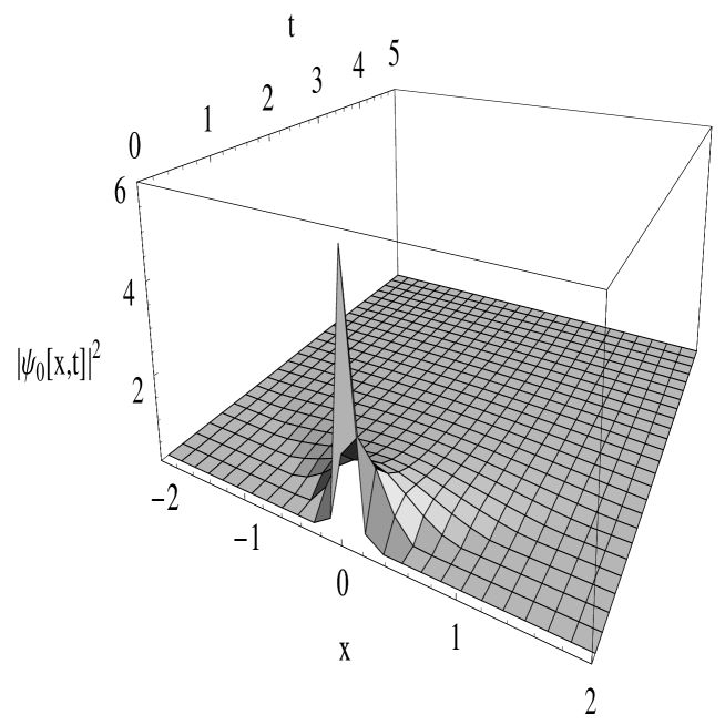
Figure 5: $|\Psi_{0}(x,t)|^{2}$ versus time and coordinate at constant mass and inverse square time frequency.

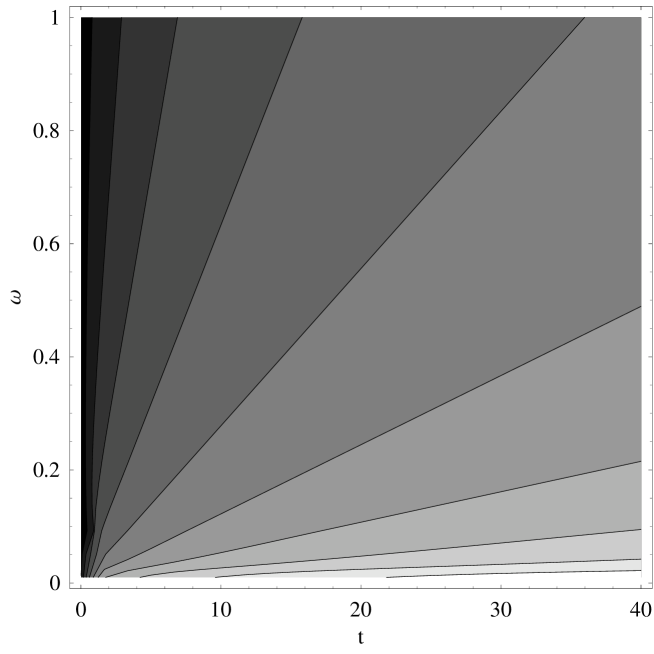
Figure 6: The counter graph of the joint entropy of Harmonic oscillator with inverse square time dependent frequency and constant mass.

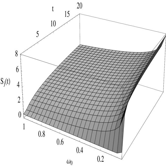
Figure 7: The 3D graph of the joint entropy of harmonic oscillator with inverse square time dependent frequency

References

- (1) E. Aydiner, C. Orta and R.Sever, E-print:quant-ph/0602203
- (2) W.H. Zurek, Phys. Today 44(10), 36 (1991).
- (3) R. Omnes, Rev. Mod. Phys. 64, 339 (1992).
- (4) C. Anastopoulos, Ann. Phys. 303, 275 (2003).
- (5) R. Leipnik, Inf. Control. 2, 64 (1959).
- (6) V.V.Dodonov, J.Opt. B: Quantum Semiclassical Opt. 4, S98 (2002).
- (7) S. A. Trigger, Bull. Lebedev Phys. Inst. 9, 44 (2004).
- (8) J. Dunkel and S. A. Trigger, Phys. Rev.A71, 052102 (2005).
- (9) P. Garbaczewski, Phys. Rev. A 72, 056101 (2005).
- (10) C. M. A. Dantas, I. A . Pedrosa and B. Baseia, Phys. Rev.A 45, 3 (1992).
- (11) R. K. Colegrave and M. S. Abdalla, Opt. Acta 28, 495 (1981).
- (12) N. A. Lemos and C. P. Natividade, Nuovo Cimento 399, 211 (1989).
- (13) Y. Ben-Aryeh and A. Mann, Pyhs. Rev. A 32, 552 (1985).
- (14) M. Born, Z. Phys. 40, 167 (1926).
- (15) R.P. Feynman, A. R. Hibbs, Quantum Mechanics and Path Integrals, McGraw-Hill, USA (1965).
- (16) D.C. Khandekar, S.V. Lawande, K.V. Bhagwat, Path-Integral Methods and Their Applications, World Scientific, Singapore (1993).
- (17) H. Kleinert, Path Integrals in Quantum Mechanics, Statistics, Polymer Physics, and Financial Markets, World Scientific, 3rd Edition (2004).
- (18) I.A. Pedrosa, Phys. Rev. A 55, 3219 (1997).
- (19) O. Ciftja, J. Phys A 32,6385 (1999).
- (20) R. K. Colegrave and M. S. Abdalla, J. Phys. A 15, 1549(1950).