Local commutativity versus Bell inequality violation for entangled states and versus non-violation for separable states

Abstract

By introducing a quantitative ‘degree of commutativity’ in terms of the angle between spin-observables we present two tight quantitative trade-off relations in the case of two qubits: First, for entangled states, between the degree of commutativity of local observables and the maximal amount of violation of the Bell inequality: if both local angles increase from zero to $\pi/2$ (i.e., the degree of local commutativity decreases), the maximum violation of the Bell inequality increases. Secondly, a converse trade-off relation holds for separable states: if both local angles approach $\pi/2$ the maximal value obtainable for the correlations in the Bell inequality decreases and thus the non-violation increases. As expected, the extremes of these relations are found in the case of anticommuting local observables where respectively the bounds of $2\sqrt{2}$ and $\sqrt{2}$ hold for the expectation value of the Bell operator. The trade-off relations show that non-commmutativity gives “a more than classical result” for entangled states, whereas “a less than classical result” is obtained for separable states. The experimental relevance of the trade-off relation for separable states is that it provides an experimental test for two qubit entanglement. Its advantages are twofold: in comparison to violations of Bell inequalities it is a stronger criterion and in comparison to entanglement witnesses it needs to make less strong assumptions about the observables implemented in the experiment.

I Introduction

In 1964, John S. Bell bell64 famously presented an inequality that holds true for all putative local hidden variable theories for a pair of spin-1/2 particles but not in quantum mechanics. In fact, this inequality is satisfied for every separable quantum state, but may be violated by any pure entangled state gisin .

It is well-known that in order to achieve such a violation one must make measurements of pairs of non-commuting spin-observables for both particles. It is also well-known (thanks to the work of Tsirelson cirelson ) that in order to achieve the maximum violation allowed by quantum theory, one must choose both pairs of these local observables to be anticommuting. It is tempting to introduce a quantitative ‘degree of commutativity’ by means of the angle between two spin-observables: if their angle is zero, the observables commute; if their angle is $\pi/2$ they anticommute, which may thought of as the extreme case of noncommutativity. Thus one may expect that there is a trade-off relation between the degrees of local commutativity and the degree of Bell inequality violation, in the sense that if both local angles increase from 0 towards $\pi/2$ (i.e., the degree of local commutativity decreases), the maximum violation of the Bell inequality increases. It is one of the purposes of this Letter to provide a quantitative tight expression of this relation for arbitrary angles.

It is less well-known that there is also a converse trade-off relation for separable states. For these states, the bound implied by the Bell inequality may be reached, but only if at least one of the pairs of local observables commute, i.e., if at least one of the angles is zero. It was shown by Roy roy (see also uffink06 ) that if both pairs anticommute, such states can only reach a bound which is considerably smaller than the bound set by the Bell inequality, namely $\sqrt{2}$ instead of $2$. Thus, for separable states there appears to be a trade-off between local commutativity and Bell inequality non-violation. The quantitative expression of this separability inequality was already investigated by Ref. roy for the special case when the local angles between the spin observables are equal. It is a second purpose of this Letter to report an improvement of this result and extend it to the general case of unequal angles. As in the case of entangled states mentioned above, the quantitative expression reported will be tight.

Apart from the pure theoretical interest of these two trade-off relations, we will show that the last one also has experimental relevance. This latter trade-off relation is a separability condition, i.e., it must be obeyed by all separable states, and consequently, a violation of this trade-off relation is a sufficient condition for the presence of entanglement. Indeed, this separability condition is strictly stronger as a test for entanglement than the ordinary Bell-CHSH inequality whenever both pairs of local observables are non-commuting (i.e., for non-parallel settings).

Furthermore, since the relation is linear in the state $\rho$ it can be easily formulated as an entanglement witness witness for two qubits in terms of locally measurable observables witness3 . It has the advantage, not shared by ordinary entanglement witnesses witness ; witness2 ; witness3 , that it is not necessary that one has exact knowledge about the observables one is implementing in the experimental procedure. Thus, even in the presence of some uncertainty about the observables measured, the tradeoff relation of this Letter allows one to use an explicit entanglement criterion nevertheless.

The structure of this Letter is as follows. Before presenting the trade-off relations in section III we will review some requisite background in section II. In section IV we will discuss the import of the relations obtained.

II Bell inequality and local commutativity

Consider a bipartite quantum system in the familiar setting of a standard Bell experiment: Two experimenters at distant sites each receive one subsystem and choose to measure one of two dichotomous observables: $A$ or $A^{\prime}$ at the first site, and $B$ or $B^{\prime}$ at the second. We assume that all observables have the spectrum $\{-1,1\}$. Define the so-called Bell operatorbraunstein

$$\mathcal{B}:=A\otimes(B+B^{\prime})+A^{\prime}\otimes(B-B^{\prime}).$$ (1)

Since $\langle\mathcal{B}\rangle_{\rho}:=\mathrm{Tr}[\mathcal{B}\rho]$ is a convex function of the quantum state $\rho$ for the system, its maximum is obtained for pure states. In fact, Tsirelsoncirelson already proved that $\max_{\rho}|\langle\mathcal{B}\rangle_{\rho}|$ can be attained in a pure two-qubit state (with associated Hilbert space $\mathcal{H}=\mathbb{C}^{2}\otimes\mathbb{C}^{2}$) and for spin observables.

In the following it will thus suffice to consider only qubits (spin-${1}/{2}$ particles) and the usual traceless spin observables, e.g. $A=\bm{a}\cdot\bm{\sigma}=\sum_{i}a_{i}\sigma_{i}$, with $\|\bm{a}\|=1$, $i=x,y,z$ and $\sigma_{x},\sigma_{y},\sigma_{z}$ the familiar Pauli spin operators on $\mathcal{H}=\mathbb{C}^{2}$.

For the set $\mathcal{D}_{\mbox{sep}}$ of all separable states, i.e., states of the form $\rho=\rho_{1}\otimes\rho_{2}$ on $\mathcal{H}=\mathbb{C}^{2}\otimes\mathbb{C}^{2}$ or convex mixtures of such states, the following Bell inequality holds, in the form derived by Clauser, Horne, Shimony and Holt chsh :

$$|\langle\mathcal{B}\rangle_{\rho}|\leq 2.$$ (2)

However, for the set $\mathcal{D}$ of all (possibly entangled) quantum states, a bound for $\langle\mathcal{B}\rangle$ is given by the Tsirelson inequality cirelson ; landau :

$$|\langle\mathcal{B}\rangle_{\rho}|\leq\sqrt{4+|\langle[A,A^{\prime}]\otimes[B,B^{\prime}]\rangle_{\rho}|}.$$ (3)

II.1 Maximal violation requires local anticommutativity

The Tsirelson inequality (3) tells us that the only way to get a violation of the Bell-CHSH inequality (2) is when both pairs of local observables are noncommuting: If one of the two commutators in (3) is zero there will be no violation of (2). Furthermore, we see from (3) that in order to maximally violate inequality (2) (i.e., to get $|\langle\mathcal{B}\rangle_{\rho}|=2\sqrt{2}$) the following condition must hold cirelson ; toner :

$$|\langle[A,A^{\prime}]\otimes[B,B^{\prime}]\rangle_{\rho}|=4.$$ (4)

The local observables $i[A,A^{\prime}]/2$ and $i[B,B^{\prime}]/2$ (which are both dichotomous and have their spectra within $[-1,1]$) must thus be maximally correlated.

However, the condition (4) is only necessary for a maximal violation, but not sufficient. Separable states are also able to obey this condition while such states never violate the Bell-CHSH inequality. For example, choose $A=B=\sigma_{y}$, $A^{\prime}=B^{\prime}=\sigma_{x}$. This gives $[A,A^{\prime}]\otimes[B,B^{\prime}]=-4\sigma_{z}\otimes\sigma_{z}$. The condition (4) is then satisfied in the separable state $(|\uparrow\uparrow\rangle\langle\uparrow\uparrow|+|\downarrow\downarrow\rangle\langle\downarrow\downarrow|)/2$ in the $z$-basis.

Nevertheless, we can infer from (4) that for maximal violation the local observables must anticommute, i.e., $\{A,A^{\prime}\}=\{B,B^{\prime}\}=0$ (a result already obtained in a different way by Popescu and Rohrlich popescu ). To see this, consider local observables, which are not necessarily anticommuting and note that $i[A,A^{\prime}]/2=-(\bm{a}\times\bm{a^{\prime}})\cdot\bm{\sigma}$ and analogously $i[B,B]/2=-(\bm{b}\times\bm{b^{\prime}})\cdot\bm{\sigma}$. We thus get

$$|\langle[A,A^{\prime}]\otimes[B^{\prime},B]\rangle_{\rho}|=4|\langle(\bm{a}\times\bm{a^{\prime}})\cdot\bm{\sigma}\otimes(\bm{b}\times\bm{b^{\prime}})\cdot\bm{\sigma}\rangle_{\rho}|.$$ (5)

This can equal 4 only if $||\,\bm{a}\times\bm{a^{\prime}}||=||\,\bm{b}\times\bm{b^{\prime}}||=1$, which implies that $\bm{a}\cdot\bm{a^{\prime}}=0$ and $\bm{b}\cdot\bm{b^{\prime}}=0$, since $\bm{a}$, $\bm{a^{\prime}}$, $\bm{b}$ and $\bm{b^{\prime}}$ are unit vectors.

If we denote by $\theta_{A}$ the angle between observables $A$ and $A^{\prime}$ (i.e., $\cos\theta_{A}=\bm{a}\cdot\bm{a^{\prime}}$) and analogously for $\theta_{B}$, we see that the local observables must thus be orthogonal: $\theta_{A}=\theta_{B}=\pi/2$ (mod $\pi$), or equivalently, they must anticommute. Thus the condition (4) implies that we need locally anticommuting observables to obtain a maximal violation of the Bell-CHSH inequality.

As mentioned in the introduction, local commutativity (i.e., $[A,A^{\prime}]=[B,B^{\prime}]=0$) corresponds to the observables being parallel or antiparallel, i.e., $\theta_{A}=\theta_{B}=0$ (mod. $\pi$), and local anticommutativity (i.e., $\{A,A^{\prime}\}=\{B,B^{\prime}\}=0$) corresponds to the observables being orthogonal, i.e., $\theta_{A},\theta_{B}=\pm\pi/2$. Therefore, in order to obtain any violation at all it is necessary that the local observables are at some angle to each other, i.e., $\theta_{A}\neq 0,\leavevmode\nobreak\ \theta_{B}\neq 0$, whereas maximal violation is only possible if the local observables are orthogonal.

This suggests that there exists a quantitative trade-off relation that expresses exactly how the amount of violation depends on the local angles $\theta_{A},\leavevmode\nobreak\ \theta_{B}$ between the spin observables. In other words, we are interested in determining the form of

$$C(\theta_{A},\theta_{B}):=\max_{\rho\in\cal{D}}|\langle\mathcal{B}\rangle_{\rho}|$$ (6)

In the next section we will present such a relation.

However, before doing so, we continue our review for the case of separable quantum states. In this case, a more stringent bound on the expectation value of the Bell operator is obtained than the usual bound of 2.

II.2 Local anticommutativity and separable states

Using the quadratic separability inequality of Ref. uffink06 for anticommutating observables ($\{A,A^{\prime}\}=\{B,B^{\prime}\}=0$) we get for all states in $\mathcal{D}_{\mbox{sep}}$:

$$\langle\mathcal{B}\rangle_{\rho}^{2}+\langle\mathcal{B}^{\prime}\rangle_{\rho}^{2}\leq 2[\langle\openone\otimes\openone- A^{\prime\prime}\otimes B^{\prime\prime}\rangle^{2}_{\rho}-$$

$$\langle A^{\prime\prime}\otimes\openone-\openone\otimes B^{\prime\prime}\rangle^{2}_{\rho}],$$ (7)

where $\mathcal{B}^{\prime}$ is the same as $\mathcal{B}$ but with the local observables interchanged (i.e., $A\leftrightarrow A^{\prime}$ , $B\leftrightarrow B^{\prime}$), and where we have also used the shorthand notation $A^{\prime\prime}=i[A,A^{\prime}]/2$ and $B^{\prime\prime}=i[B,B^{\prime}]/2$. Note that the triple $A,A^{\prime},A^{\prime\prime}$ are mutually anticommuting and can thus be easily extended to form a set of local orthogonal observables for $\mathbb{C}^{2}$ (so-called LOO’s witness2 ).

The separability inequality (II.2) provides a very strong entanglement criterion uffink06 , but it is here used to derive a (weaker) separability inequality in terms of the Bell operator $\mathcal{B}$ for all states in $\mathcal{D}_{\mbox{sep}}$:

$$|\langle\mathcal{B}\rangle_{\rho}|\leq\sqrt{2(1-\frac{1}{4}|\langle[A,A^{\prime}]\rangle_{\rho_{1}}|^{2})(1-\frac{1}{4}|\langle[B,B^{\prime}]\rangle_{\rho_{2}}|^{2})}.$$ (8)

Here $\rho_{1}$ and $\rho_{2}$ are the reduced single qubit states that are obtained from $\rho$ by partial tracing over the other qubit. The inequality (8) is the separability analogue for anticommuting observables of the Tsirelson inequality (3). Note that even in the weakest case ($\langle[A,A^{\prime}]\rangle_{\rho_{1}}=\langle[B,B]\rangle_{\rho_{2}}=0$) it implies $|\langle\mathcal{B}\rangle_{\rho}|\leq\sqrt{2}$, which strengthens the original Bell-CHSH inequality voetnoot1 . Thus, for separable states, a reversed effect of the requirement of local anticommutativity appears than for entangled quantum states. Indeed, for locally anticommuting observables we deduce from (8) that the maximum value of $\langle\mathcal{B}\rangle_{\rho}$ is considerably less than the maximum value of $2$ attainable using commuting observables. In contrast to entangled states, the requirement of anticommutivity, which, as we have seen, is equivalent to local orthogonality of the spin observables, thus decreases the maximum expectation value of the Bell operator $\mathcal{B}$ for separable states.

An interesting question is now: what happens to the maximum attainable by separable states for locally noncommuting observables that are not precisely anticommuting? Or put equivalently, how does this bound depend on the angles between the local spin observables when the observables are neither parallel nor orthogonal? From the above one would expect the bound to drop below the standard bound of $2$ as soon as the settings are not parallel or anti-parallel. Just as in the case of general quantum states it would thus be interesting to get a quantitative trade-off relation that expresses exactly how the maximum bound for $\langle\mathcal{B}\rangle_{\rho}$ depends on the local angles of the spin observables. In other words, we need to establish

$$D(\theta_{A},\theta_{B}):=\max_{\rho\in\cal{D}_{\mbox{\scriptsize sep}}}|\langle\mathcal{B}\rangle_{\rho}|,$$ (9)

from which we obtain the separability inequality

$$|\langle\mathcal{B}\rangle_{\rho}|\leq D(\theta_{A},\theta_{B}),\leavevmode\nobreak\ \leavevmode\nobreak\ \leavevmode\nobreak\ \rho\in\cal{D}_{\mbox{\scriptsize sep}}.$$ (10)

In the following we present such a tight trade-off relation.

III Trade-off relations

III.1 General qubit states

It was already pointed out by Landau landau that inequality (3) is tight, i.e., for all choices of the observables, there exists a state $\rho$ such that :

$$\max_{\rho\in\mathcal{D}}|\langle\mathcal{B}_{\rho}\rangle|=\sqrt{4+|\langle[A,A^{\prime}]\otimes[B^{\prime},B]\rangle_{\rho}|}.$$ (11)

This maximum is invariant under local unitary transformations $U\otimes U^{\prime}$, since Tr$[(U\otimes U^{\prime})^{\dagger}\mathcal{B}(U\otimes U^{\prime})\rho]=$ Tr$[\mathcal{B}\tilde{\rho}]$ with $\tilde{\rho}=(U\otimes U^{\prime})\rho(U\otimes U^{\prime})^{\dagger}$. This invariance amounts to a freedom in the choice of the local reference frames.

Hence, without loss of generality, we can choose

$$\bm{a}=(1,0,0),\leavevmode\nobreak\ \bm{a^{\prime}}=(\cos\theta_{A},\sin\theta_{A},0),$$

$$\bm{b}=(1,0,0),\leavevmode\nobreak\ \bm{b^{\prime}}=(\cos\theta_{B},\sin\theta_{B},0).$$ (12)

For this choice (12) one has $i[A,A^{\prime}]/2=-\sin\theta_{A}\leavevmode\nobreak\ \sigma_{z}$ and, analogously, $i[B,B]/2=-\sin\theta_{B}\leavevmode\nobreak\ \sigma_{z}$. Hence, we immediately obtain

$$\max_{\rho\in\mathcal{D}}|\langle\mathcal{B}_{\rho}\rangle|=\sqrt{4+4|\sin\theta_{A}\sin\theta_{B}\langle\sigma_{z}\otimes\sigma_{z}\rangle_{\rho}|}.$$ (13)

To obtain a state independent bound, it remains to be shown that we can choose $\rho$ such that $|\langle\sigma_{z}\otimes\sigma_{z}\rangle_{\rho}|=1$ in order to conclude that

$$C(\theta_{A},\theta_{B})=\sqrt{4+4|\sin\theta_{A}\sin\theta_{B}|}.$$ (14)

To see that (14) holds, note that the Bell operator for the above choice (12) of observables becomes:

$$\mathcal{B}=\alpha|\uparrow\uparrow\rangle\langle\downarrow\downarrow|+\beta|\uparrow\downarrow\rangle\langle\downarrow\uparrow|+\alpha^{*}|\downarrow\uparrow\rangle\langle\uparrow\downarrow|+\beta^{*}|\downarrow\downarrow\rangle\langle\uparrow\uparrow|,$$ (15)

with

$$\alpha = 1+e^{-i\theta_{A}}+e^{-i\theta_{B}}-e^{-i(\theta_{A}+\theta_{B})},$$ (16)

$$\beta = 1+e^{-i\theta_{A}}+e^{i\theta_{B}}-e^{-i(\theta_{A}-\theta_{B})}.$$ (17)

We distinguish two cases: (i) when $\sin\theta_{A}\sin\theta_{B}\geq 0$ (i.e. when $0\leq\theta_{A},\theta_{B}\leq\pi$ or $\pi\leq\theta_{A},\theta_{B}\leq 2\pi$), choose the pure state $|\phi_{\tau}^{+}\rangle=\frac{1}{\sqrt{2}}(|\uparrow\uparrow\rangle+e^{i\tau}|\downarrow\downarrow\rangle)$. Then:

$$\max_{\tau}\, \mathrm{Tr}[\mathcal{B}|\phi_{\tau}^{+}\rangle\langle\phi_{\tau}^{+}|]=\max_{\tau}[\mathrm{Re}(\alpha)\cos\tau+\mathrm{Im}(\alpha)\sin\tau]$$

$$=|\alpha|=\sqrt{4+4\sin\theta_{A}\sin\theta_{B}}.$$ (18)

Similarly, (ii) for $\sin\theta_{A}\sin\theta_{B}\leq 0$ (i.e., $0\leq\theta_{A}\leq\pi$, $\pi\leq\theta_{B}\leq 2\pi$ or $\pi\leq\theta_{A}\leq 2\pi$, $0\leq\theta_{B}\leq\pi$), and the pure state $|\psi_{\tau}^{+}\rangle=\frac{1}{\sqrt{2}}(|\uparrow\downarrow\rangle+e^{i\tau}|\downarrow\uparrow\rangle)$ we find

$$\max_{\tau}\, \mathrm{Tr}[\mathcal{B}|\psi_{\tau}^{+}\rangle\langle\psi_{\tau}^{+}|]=\max_{\tau}[\mathrm{Re}(\beta)\cos\tau+\mathrm{Im}(\beta)\sin\tau]$$

$$=|\beta|=\sqrt{4-4\sin\theta_{A}\sin\theta_{B}}.$$ (19)

Since $|\langle\sigma_{z}\otimes\sigma_{z}\rangle_{\phi_{\tau}^{+}}|=|\langle\sigma_{z}\otimes\sigma_{z}\rangle_{\psi_{\tau}^{+}}|=1$ we see that the bound in (14) is saturated. The shape of the function $C(\theta_{A},\theta_{B})$ as determined in (14) is plotted in Figure 1.

We thus see that $C(\theta_{A},\theta_{B})$ becomes greater and greater when the angles approach orthogonality. Obviously, for the extreme cases of parallel and completely orthogonal settings (i.e., $\theta_{A}=\theta_{B}=0$ or $\pi/2$) we retrieve the results mentioned in section II.1.

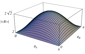
Figure 1: Plot of $C(\theta_{A},\theta_{B})=\max_{\rho\in\cal{D}}|\langle\mathcal{B}\rangle_{\rho}|$ as given in (14) for $0\leq\theta_{A},\theta_{B}\leq\pi$.

If both angles are chosen the same, i.e., $\theta_{A}=\theta_{B}:=\theta$, (14) simplifies to

$$C(\theta,\theta)=\sqrt{4+4\sin^{2}\theta},$$ (20)

which is plotted in Figure 3.

III.2 Separable qubit states

The set $\mathcal{D}_{\mbox{\scriptsize sep}}$ of separable states is closed under local unitary transformations. Therefore, to find $\max_{\rho\in\mathcal{D}_{\mbox{\tiny sep}}}|\langle\mathcal{B}\rangle_{\rho}|$, we may consider the same choice of observables as before in (12) without loss of generality. Further, we only have to consider pure states and can take the state $|\Psi\rangle=|\psi_{1}\rangle|\psi_{2}\rangle$ with $|\psi_{1}\rangle=\cos\gamma_{1}e^{-i\phi_{1}/2}|\uparrow\rangle+\sin\gamma_{1}e^{i\phi_{1}/2}|\downarrow\rangle$ and $|\psi_{2}\rangle=\cos\gamma_{2}e^{-i\phi_{2}/2}|\uparrow\rangle+\sin\gamma_{2}e^{i\phi_{2}/2}|\downarrow\rangle$. We then obtain $\langle A\rangle_{\psi_{1}}=\sin 2\gamma_{1}\cos\phi_{1}$, $\langle A^{\prime}\rangle_{\psi_{1}}=\sin 2\gamma_{1}\cos(\phi_{1}-\theta_{A})$, $\langle B\rangle_{{\psi_{2}}}=\sin 2\gamma_{2}\cos\phi_{2}$ and $\langle B^{\prime}\rangle_{{\psi_{2}}}=\sin 2\gamma_{2}\cos(\phi_{2}-\theta_{B}).$

Since $|\Psi\rangle$ is separable, we get $\langle A\otimes B\rangle_{\Psi}=\langle A\rangle_{{\psi_{1}}}\langle B\rangle_{{\psi_{2}}}$, etc., and the maximal expectation value of the Bell operator becomes

$$D( \theta_{A},\theta_{B})=\max_{{\Psi}}\,\langle\mathcal{B}\rangle_{\Psi}$$

$$=\max_{\gamma_{1},\gamma_{2},\phi_{1},\phi_{2}}\sin 2\gamma_{1}\sin 2\gamma_{2}[\cos\phi_{1}(\cos\phi_{2}+\cos(\phi_{2}-\theta_{B}))$$

$$\leavevmode\nobreak\ \leavevmode\nobreak\ \leavevmode\nobreak\ \leavevmode\nobreak\ +\cos(\phi_{1}-\theta_{A})(\cos\phi_{2}-\cos(\phi_{2}-\theta_{B}))].$$ (21)

This maximum is attained for $\gamma_{1}=\gamma_{2}=\pi/4$ and (21) reduces to:

$$D(\theta_{A},\theta_{B})= \max_{\phi_{1},\phi_{2}}\,\cos\phi_{1}(\cos\phi_{2}+\cos(\phi_{2}-\theta_{B}))$$

$$+\cos(\phi_{1}-\theta_{A})(\cos\phi_{2}-\cos(\phi_{2}-\theta_{B})).$$ (22)

A tedious but straightforward calculation yields that the maximum over $\phi_{1}$ and $\phi_{2}$ is given by

$$D(\theta_{A},\theta_{B})= \Big{|}\mathrm{W}_{+}(1+\mathrm{X}_{\pm}^{2})^{-1/2}$$

$$+\mathrm{cos}(\mathrm{arctan}(\mathrm{X}_{\pm})-\theta_{A})\,\mathrm{W}_{-}\Big{|},$$ (23)

with

$$\mathrm{W}_{\pm}: =(1+\frac{\mathrm{Z}^{2}}{\mathrm{sin}^{2}\theta_{B}\,\mathrm{Y}^{2}})^{-1/2}$$

$$\pm\mathrm{cos}(\mathrm{arctan}({\frac{\mathrm{Z}}{\mathrm{sin}\theta_{B}\,\mathrm{Y}}})+\theta_{B}),$$ (24)

$$\mathrm{X}_{\pm}: =(\sin\theta_{A}\cos^{2}\theta_{A}\sin^{2}\theta_{B})^{-1}\big{(}-\cos\theta_{A}(\cos\theta_{B}$$

$$+\cos^{2}\theta_{B}+\cos^{2}\theta_{A}\sin^{2}\theta_{B})\pm(\cos^{2}\theta_{A}$$ (25)

$$\times(1+\cos^{2}\theta_{B})(\cos^{2}\theta_{B}+\cos^{2}\theta_{A}\sin^{2}\theta_{B}))^{1/2}\big{)}$$

$$\mathrm{Y}: =\mathrm{X}_{\pm}(1-\cos\theta_{A}+\sin\theta_{A}),$$ (26)

$$\mathrm{Z}: =\mathrm{X}_{\pm}(1+\cos\theta_{B}+\cos\theta_{A}-\cos\theta_{B}\,\cos\theta_{A})+$$

$$\cos\theta_{B}\sin\theta_{A}-\sin\theta_{A},$$ (27)

where in $\mathrm{X}_{\pm}$ the $+$ sign is chosen for $-\pi/2\leq\theta_{A}\leq\pi/2$ and the $-$ sign is chosen for $\pi/2\leq\theta_{A}\leq 3\pi/2$ (both modulo $2\pi$). The function (23) is plotted in Figure 2.

From this figure we conclude that the maximum of $|\langle\mathcal{B}\rangle_{\rho}|$ for separable states becomes smaller and smaller when the angles approach orthogonality. For parallel and completely orthogonal settings we again retrieve the results of section II.2.

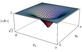
Figure 2: Plot of $D(\theta_{A},\theta_{B}):=\max_{\rho\in\cal{D}_{\mbox{\scriptsize sep}}}|\langle\mathcal{B}\rangle_{\rho}|$ as given in (23) for $0\leq\theta_{A},\theta_{B}\leq\pi$.

As a special case, suppose we choose $\theta_{A}=\theta_{B}:=\theta$. Then, (23) reduces to the much simpler expression

$$D(\theta,\theta)=|\cos\theta|+\sqrt{1+\sin^{2}\theta}.$$ (28)

This result strengthens the bound obtained previously by Roy roy for this special case, which is:

$$D(\theta,\theta)\leq\left\{\begin{array}[]{ll}\sqrt{2}(|\cos\theta|+1),&|\cos\theta|\leq 3-2\sqrt{2},\\ 1+2\sqrt{|\cos\theta|}-|\cos\theta|,&\leavevmode\nobreak\ \leavevmode\nobreak\ \mathrm{otherwise}.\end{array}\right.$$ (29)

Both functions are shown in Figure 3.

Figure 3: Plot of the results (20) (dashed line) and (28) (uninterupted line), and of the bound by Roy roy given in (29) (dotted line).

IV Discussion

In this letter we have given tight quantitative expressions for two trade-off relations. Firstly, between the degrees of local commutativity, as measured by the local angles $\theta_{A}$ and $\theta_{B}$, and the maximal degree of Bell-CHSH inequality violation, in the sense that if both local angles increase towards $\pi/2$ (i.e., the degree of local commutativity decreases), the maximum violation of the Bell-CHSH inequality increases. Secondly, a converse trade-off relation holds for separable states: if both local angles increase towards $\pi/2$, the value attainable for the expectation of the Bell operator decreases and thus the non-violation of the Bell-CHSH inequality increases. The extreme cases of these relations are obtained for anticommuting local observables where the bounds of $2\sqrt{2}$ and $\sqrt{2}$ hold. For the case of equal angles the trade-off relation for separable states strengthens a previous result of Royroy .

Our results are complementary to the well studied question what the maximum of the expectation value of the Bell operator is when evaluated in a certain state (see e.g., gisin ). Here we have not focussed on a certain given state, but instead on the observables chosen, i.e., we asked, independent of the specific state of the system, what the maximum of the expectation value of the Bell operator is when using certain local observables. The answer found shows a diverging trade-off relation for the two classes of separable and non-separable states.

Indeed, these two trade-off relations show that local noncommutativity has two diametrically opposed features: On the one hand, the choice of locally non-commuting observables is necessary to allow for any violation of the Bell-CHSH inequality in entangled states (a “more than classical” result). On the other hand, this very same choice of non-commuting observables implies a “less than classical” result for separable states: For such states the correlations (in terms of $\langle\mathcal{B}\rangle_{\rho}$) obey a more stringent bound than allowed for in local hidden variable theories, i.e. the Bell-CHSH inequality (2).

These trade-off relations are useful for experiments aiming to detect entangled states. They have an experimental advantage above both Bell inequalities and entanglement witnesses as tests for two qubit entanglement. This will be discussed next.

For comparison to the Bell-CHSH inequality as a test of entanglement, let us define the ’violation factor’ $X$ as the ratio $C(\theta_{A},\theta_{B})/D(\theta_{A},\theta_{B})$, i.e. the maximum correlation attained by entangled states divided by the maximum correlation attainable for separable states. In Figure (4) we have plotted this violation factor $X$ for the special case of equal angles, cf. (20) and (28) and compared it to the ratio by which these maximal correlations violate the Bell-CHSH inequality (2), i.e. $X_{\mathrm{CHSH}}:=C(\theta,\theta)/2$. Figure 4 shows that the violation factor $X$ is always higher than $X_{\rm CHSH}$ except when $\theta=0$. For angles $\theta\lesssim\pi/4$ these two factors differ only slightly, but the violation factor $X_{\mathrm{}}$ increases to $\sqrt{2}$ times the original factor $X_{\mathrm{CHSH}}$ when $\theta$ approaches $\pi/2$. Furthermore note that the factor $X_{\mathrm{}}$ increases more and more steeply, whereas $X_{\mathrm{CHSH}}$ increases less and less steeply. For the case of unequal angles the same features occur, as is evident from comparing Figures 1 and 2.

Figure 4: Violation factor $X$ (uninterupted line) and $X_{\mathrm{CHSH}}$ (dashed line) for $\theta_{A}=\theta_{B}:=\theta$.

Therefore, the comparison of the correlation in entangled states to the maximum correlation obtainable in separable states yields a stronger test for entanglement than violations of the Bell-CHSH inequality. Indeed, the violation factor may reach 2 instead of $\sqrt{2}$. This means that the separability inequality (10) allows for detecting more entangled states as well as for greater noise robustness in detecting entanglement (cf. uffink06 ). Clearly, the optimal case of this relation obtains when the local observables are exactly orthogonal to each other. On the other hand, in the case where at least one of the local pairs of observables are parallel, no improvement upon the Bell-CHSH inequality is obtained. But that case is trivial, i.e., no entangled state can violate either (2) or (10) in that case.

Other criteria for the detection of entanglement than the Bell-CHSH inequality have been developed in the form of entanglement witnesses. In general, these criteria have two experimental drawbacks voetnoot2 : (i) they are usually designed for the detection of a particular entangled state and hence require some a priori knowledge about the state, and (ii) they require the implementation of a specific set of local observables (e.g., locally orthogonal ones witness2 ). The separability inequality (10) compares favorably on these two points, as we will discuss next.

In real experimental situations one might not be completely sure about which observables are being measured. For example, one might not be sure that the local angles are exactly orthogonal in the optimal setup. However, even in such cases, one might be reasonably sure that the angles are close to 90 degrees, e.g., that these angles certainly lie within some finite-sized interval $\epsilon$ around 90 degrees. In that case, the bound (10) for separable states would of course be higher than the optimal value of $\sqrt{2}$ and the increase depends on the size of the interval specified. But the trade-off relation presented in this letter tells us exactly how much higher the bound becomes as a function of the angles (e.g., $\theta=\pi/2\pm\epsilon$), so one can still obtain a relevant bound on $|\langle\mathcal{B}\rangle|$. One can thus still use it as a criterion for testing entanglement in the presence of some ignorance about the measured observables. Entanglement witnesses do not share this feature since no other trade-off relations have been obtained (at least to our knowledge) that quantify how the performance of the witness is changed when one allows for uncertainty in the observables that feature in the witness.

Note that for two qubits this result answers the question raised in Ref. nagata where it was asked how separability inequalities for orthogonal observables could allow for some uncertainty $\epsilon$ in the orthogonality, i.e., allowing for $|\{A,A^{\prime}\}|\leq\epsilon$ (analogous for $B$, $B^{\prime}$).

A further advantage of the separability inequalities (10) is that they are not state-dependent and are formulated in terms of locally measurable observables from the start, whereas it is usually the case (apart from a few simple cases) that constructions of entanglement witnesses involve some extremization procedure and are state-dependent. Furthermore, finding the decomposition of witnesses in terms of a few locally measurable observables is not always easy witness3 . However, it must be said that choosing the optimal set of observables in the separability inequalities for detecting a specific state of course also requires some prior knowledge of this state.

The results presented here only concern the bipartite linear Bell-type inequality. It might prove useful to look for similar trade-off relations for nonlinear separability inequalities as well as for entanglement witnesses. Furthermore, it would be interesting to extend this analysis to the multipartite Bell-type inequalities involving two dichotomous observables per party such as the Werner-Wolff-Żukowski-Brukner inequalities werner or the Mermin-type inequalities mrskab . For the latter the situation for local anticommutivity has already been investigated roy ; nagata ; seevinck06 , but for non-commuting observables that are not anticommuting no results have yet been obtained.

References

- (1) J.S. Bell, Physics 1, 195 (1964).
- (2) N. Gisin, Phys. Lett. A 154, 201 (1991). N. Gisin and A. Peres, Phys. Lett. A 162, 15 (1992). S. Popescu and D. Rohrlich, Phys. Lett. A 166, 293 (1992).
- (3) B.S. Cirel’son, Lett. Math. Phys. 4, 93 (1980).
- (4) S.M. Roy, Phys. Rev. Lett. 94, 010402 (2005).
- (5) J. Uffink and M. Seevinck, to be published in Phys. Lett A. Quant-ph/0604145 (2006).
- (6) M. Horodecki, P. Horodecki and R. Horodecki,Phys. Lett. A 223, 1 (1996). B.M.Terhal, Phys. Lett. A 271, 319 (1996); M. Lewenstein, B. Kraus, J.I. Cirac and P. Horodecki, Phys. Rev. A 62, 052310 (2000). D. Bruß et al., J. Mod. Opt. 49, 1399 (2002).
- (7) O. Gühne et al., J. Mod. Opt. 50, 1079 (2003). O. Gühne et al., Phys. Rev. A. 66, 062305 (2002). B. M. Terhal, J. Theor. Comput. Sci. 287, 313 (2002)
- (8) O. Gühne, M. Mechler, G. Tóth and P. Adam Phys. Rev. A 74, 010301(R) (2006); S. Yu and N.-L. Liu, Phys. Rev. Lett. 95 150504 (2005); Zhang, et al., Phys. Rev A. 76, 012334 (2007).
- (9) S.L. Braunstein, A. Mann and M.Revzen, Phys. Rev. Lett. 68, 3259 (1992).
- (10) J.F. Clauser, M.A. Horne, A. Shimony and R.A. Holt, Phys. Rev. Lett. 26, 880 (1969).
- (11) L.J. Landau, Phys. Lett. A 120, 54 (1987).
- (12) B.F. Toner, F. Verstraete, quant-ph/0611001 (2006).
- (13) S. Popescu and D. Rohrlich, Phys. Lett. A 169, 411 (1992).
- (14) See Ref. uffink06 for a discussion of how these separability inequalities relate to local realism.
- (15) See also Ref. enk where the assumptions needed in various entanglement verification procedures are extensively discussed.
- (16) S.J. van Enk, N. Lütkenhaus and H.J. Kimble, Phys. Rev. A 75,052318 (2007).
- (17) K. Nagata, M. Koashi and N.Imoto, Phys. Rev. Lett. 89, 260401 (2002).
- (18) R.F. Werner, M.M. Wolf, Phys. Rev. A 64, 032112 (2002). M. Żukowski and Č. Brukner, Phys. Rev. Lett. 88, 210401 (2002).
- (19) N.D. Mermin, Phys. Rev. Lett. 65, 1838 (1990); S.M. Roy, V. Singh, Phys. Rev. Lett. 67, 2761 (1991); M. Ardehali, Phys. Rev. A 46, 5375 (1992); A.V. Belinskiĭ, D.N. Klyshko, Phys. Usp. 36, 653 (1993).
- (20) M. Seevinck and J. Uffink, in preparation.