Geometric Phases and Critical Phenomena in a Chain of Interacting Spins

Abstract

The geometric phase can act as a signature for critical regions of interacting spin chains in the limit where the corresponding circuit in parameter space is shrunk to a point and the number of spins is extended to infinity; for finite circuit radii or finite spin chain lengths, the geometric phase is always trivial (a multiple of $2\pi$). In this work, by contrast, two related signatures of criticality are proposed which obey finite-size scaling and which circumvent the need for assuming any unphysical limits. They are based on the notion of the Bargmann invariant whose phase may be regarded as a discretized version of Berry’s phase. As circuits are considered which are composed of a discrete, finite set of vertices in parameter space, they are able to pass directly through a critical point, rather than having to circumnavigate it. The proposed mechanism is shown to provide a diagnostic tool for criticality in the case of a given non-solvable one-dimensional spin chain with nearest-neighbour interactions in the presence of an external magnetic field.

I Introduction

I.1 Quantum Phase Transitions

Unlike ordinary phase transitions, quantum phase transitions (QPTs) Vojta take place at a temperature of absolute zero and are consequently driven entirely by quantum fluctuations, rather than thermal ones. Moreover, the long-range, algebraically decaying correlations which are characteristic of critical many-body ground states are due entirely to entanglement. As such, one would expect entanglement measures (see Ref. EntMeasures for an overview) to provide further insight into the fundamental physical underpinnings of QPTs, possibly complementing the conventional condensed-matter approach, which relies mostly on two-point correlation functions.

Indeed, Osterloh and co-workers OsterlohEtAl demonstrated singular and scaling behaviour of a bipartite entanglement measure in the vicinity of the critical point in the one-dimensional XY spin model. On the other hand, this behaviour could be understood entirely from that of the relevant two-point correlation functions as these are sufficient to determine the two-particle reduced density matrices. Furthermore, the entanglement between just two sites is not particularly well suited to capturing the large-scale behaviour of correlations, which becomes all the more relevant in the critical regime. This was recognized in Ref. BlockEntIC , where the scaling behaviour of the entanglement between a contiguous block of $L$ sites with the rest of the lattice was first considered in lattice field theories. It was found that the entanglement entropy of noncritical chains with short-ranged interactions reaches a saturation level, while the entanglement entropy diverges logarithmically with $L$ in the field limit, i.e. in the case of critical chains. This approach was subsequently pursued numerically VidalLatorre in the particular context of the one-dimensional XY model and, in more generality, in an analytical treatment based on random matrix theory Keating , applicable to any spin chain Hamiltonian that can be cast into a quadratic form of fermionic operators.

At the same time, progress has been hampered by the realization that bi-partite entanglement, whether of blocks of spins or otherwise, at best only gives us an incomplete, local picture of the entanglement exhibited by generic many-body ground states. It is something of a truism, of course, to note that a truly global, multi-partite approach is indispensable if one wishes to capture the entanglement that pervades critical many-body ground states simultaneously at all length scales (for recent work on multi-partite entanglement in quantum spin chains see for example Refs. Bruss ; Costantini ).

Unfortunately, the theory of multi-partite entanglement is still very much in its infancy. It is true that many of the entanglement measures used for bi-partite states carry straightforward generalizations to the multi-partite setting. This is particularly true for distance-based entanglement measures, such as the relative entropy of entanglement RelEnt or the closely related geometric entanglement Geometric : the entanglement of a state is then simply quantified in terms of the minimum distance of that state from the set of all multi-partite separable states, rather than the set of all bi-partite separable states. However, it is one thing to generalize the axiomatic definitions of entanglement measures to include the multi-partite case, but quite another to still be able to compute these in practice. Moreover, the theory of multi-partite entanglement is still plagued by a host of different candidates for suitable entanglement measures, even for the case of pure states (see Ref. EntMeasures for more details).

In view of these difficulties, attention has shifted to include other, potentially related, means of characterizing QPTs Zanardi . One such approach centres around the notion of geometric phase Berry ; Resta ; Carollo1 ; Carollo2 ; Hamma , and it is this approach which we wish to pursue in the remainder of this work.

I.2 Geometric Phase

In his seminal paper Berry , Berry investigated the phase picked up by an eigenstate of a parameter-dependent Hamiltonian when transported adiabatically around a closed trajectory in parameter space. It turns out that in addition to the well-known dynamical phase there is also a geometric component to the phase, which is observable, at least in principle. While the dynamical phase provides a measure of the duration of the Hamiltonian’s evolution and is independent of the geometry of the trajectory followed, conversely, the geometric phase is independent of the rate at which the state is transported around the loop (as long as this is slow enough for the adiabatic theorem to rule out transitions to neighbouring, orthogonal states) and depends solely upon the geometry of the trajectory. The geometric phase had hitherto been widely overlooked as just another unphysical phase factor, and certainly had not been granted the level of recognition it enjoys nowadays.

Before going on to explain how Berry’s phase may be used to probe for QPTs, it is useful here to first restate a simple example given in Berry’s original paper, which serves to illustrate the concept of geometric phase. To that end, consider a single spin-$1/2$ particle which is coupled to an external magnetic field, and suppose the spin is initially aligned with the magnetic field, i.e. the particle is in an eigenstate of the system’s Hamiltonian. Then the spin will remain aligned with the magnetic field vector (the particle remains in the instantaneous eigenstate) when the magnetic field vector is made to rotate adiabatically. Upon completion of some closed trajectory, the final state of the particle differs from its initial one by an overall phase factor, which is part dynamical, part geometric in origin. Now, it turns out that the geometric phase is in fact equal in size to precisely half the solid angle subtended at the origin by the magnetic field vector’s trajectory in parameter space. This result not only serves to highlight in a particularly acute way the geometric character of Berry’s phase, but it also gives an indication of the origin of Berry’s phase: the spin’s state is degenerate when the magnetic field is switched off, and the geometric phase can thus be interpreted as providing a measure of the view of the circuit as seen from that point of degeneracy at the origin of the parameter space.

In fact, in any general setting, the emergence of geometric phases can always be traced back to the presence of isolated singularities in parameter space. Formally, Berry’s phase can be related to the curvature of the Hilbert space bundle over the base space of parameters Simon , and it is this interpretation of Berry’s phase which renders its potential usefulness as a diagnostic tool for criticality plausible: points of degeneracy are associated with a greater curvature of the associated Hilbert space bundle, and therefore it might be reasonable to expect Berry’s phase to act as a signature for quantum critical points in interacting spin systems.

Of course, the geometric phase of $N$ non-interacting spin-$1/2$ particles with respect to a particular circuit is simply $N$ times the geometric phase of a single particle, which in turn can be related to the circuit’s solid angle, as explained above. However, as we switch on the spin-spin interactions, this simple interpretation of the geometric phase in terms of solid angles starts to break down. It is of great interest to know how the geometric phase of a set of interacting spins with respect to a given circuit changes as a function of the coupling parameter, and whether the geometric phase is able to signal the presence of critical points in the system. An important point to note here is that the circuit in parameter space need only pass near the critical point for the Berry phase to register it. In other words, the system need not actually undergo the quantum phase transition for the Berry phase to pinpoint its presence and location in parameter space, a consideration which assumes particular importance in the light of the difficulties that may be associated with physically implementing actual QPTs.

I.3 Previous Work

A relationship between the geometric phase and criticality in spin chains was examined by Carollo and Pachos Carollo1 ; Carollo2 . Specifically, the authors analyzed the Berry phase of the ground state of a one-dimensional spin-$1/2$ $XY$ model

$$H=\sum_{l=-M}^{M}\left(\frac{1+\gamma}{2}\sigma_{l}^{x}\sigma_{l+1}^{x}+\frac{1-\gamma}{2}\sigma_{l}^{y}\sigma_{l+1}^{y}+\lambda\sigma_{l}^{z}\right),$$ (1)

where $M=(N-1)/2$ for an odd number of spins $N$. The Berry phase, as computed with respect to a rotation of the complete Hamiltonian around the $z$-axis, was shown to exhibit the following property in the thermodynamical limit $N\rightarrow\infty$:

$$\lim_{\gamma\rightarrow 0}(\varphi/M)=\begin{cases}0\,(\text{mod }2\pi),&\text{for}|\lambda|>1\\ \text{finite},&\text{for}|\lambda|<1.\end{cases}$$

As the $XY$ model is critical for $|\lambda|<1$ (and non-critical otherwise), the quantity given above may be interpreted as a signature of criticality for this model. Unfortunately, the Berry phase per spin, $\varphi/M$, is not a physical quantity that is accessible via experiments. We can only measure the total Berry phase $\varphi$, which vanishes for all values of $\lambda$: i.e. $(1/M)\lim_{\gamma\rightarrow 0}\varphi=0\,(\text{mod }2\pi),\forall\lambda$. This is in agreement with Hamma Hamma , who also showed, via a different line of argument, that for a finite number of spins, the Berry phase acquired by the ground state is always trivial ($0$ or $2\pi$). As an alternative, it was suggested that the same quantity would be non-trivial in the thermodynamic limit: $\lim_{\gamma\rightarrow 0}\lim_{M\rightarrow\infty}(\varphi/M)\neq 0$. However, for any physical, finite system, no matter how large, one is not able to detect criticality in this manner. In other words, any finite-size scaling behaviour is completely lacking, i.e. $\lim_{M\rightarrow\infty}\lim_{\gamma\rightarrow 0}(\varphi/M)=0\,\mbox{(mod 2$\pi$)}$; it is only in the thermodynamic limit itself that this method represents a signature of criticality, i.e. the limiting case is reached discontinuously. As such, the result’s worth is perhaps more of an abstract, mathematical nature, than of any real, physically measurable consequence.

In the present work, in contrast, we employ a technique based on the geometric phase that is able to detect critical points without the need to contract the circuit’s radius to zero or to extend the number of particles to infinity. We do so by considering discretized circuits that pass directly through the critical point, rather than circumnavigating it. This procedure and the obtained results are outlined in the following.

II Procedure and Outline

We start by introducing the concept of a Bargmann invariant Bargmann and its associated phase, which may be regarded as a generalized Berry phase. It will be seen that Bargmann invariants are ideally suited for numerically analyzing the gauge-invariant phase induced by evolving states along a discretized circuit in parameter space. We then introduce the model of interacting spin-$1/2$ particles with which we will be concerned for the rest of this paper and discuss some of its more salient features. The Bargmann invariant and associated phase is computed numerically for a chosen discretized circuit and plotted as a function of the spin coupling strength $J$. Of note will be the ‘speed’ (to be defined) with which the Bargmann invariant changes as a function of $J$ and the behaviour of the magnitude of the Bargmann invariant; we will find that both of these quantities can act as adequate signatures of criticality. At this stage, it may be helpful to depict the procedure schematically:

\psfrag{A}[tc][tc]{$J$}\psfrag{B}[tc][tc]{$J_{c}$}\psfrag{Sn}[bl][bl]{$\underline{\alpha}_{\mathcal{N}}=\underline{\alpha}_{0}$}\psfrag{SS}[rc][rc]{$\underline{\alpha}_{s+1}$}\psfrag{SS1}[rc][rc]{$\underline{\alpha}_{s}$}\includegraphics[width=164.77771pt]{schematic}

Figure 1: A schematic representation of the procedure used to compute the Bargmann invariant with respect to some chosen circuit $\{\underline{\alpha}_{s}\}$ in parameter space, as a function of the spin coupling strength $J$.

Let us fix the coupling parameter to some value $J_{0}$ and choose a particular circuit composed of $\mathcal{N}$ vertices $\underline{\alpha}_{s}$, each representing the set of parameters needed (together with $J_{0}$) in order to completely describe the Hamiltonian of the system at that point. At each individual point on the circuit we numerically compute the ground state of the system. The Bargmann invariant associated with the circuit at $J_{0}$ is then obtained by cyclically multiplying successive overlaps of these ground state wavefunctions. This will be explained in more detail in section III, which is devoted entirely to the subject of Bargmann invariants; for now, we merely note that, in order to be sure to acquire a gauge-invariant quantity in this way, the wavefunctions at the start and end points of the circle need to be taken as identical. By repeating this procedure for a range of different coupling strengths (generating a complex number, the Bargmann invariant, for each value), we start to build up a picture of the general trend. We present our results for varying lengths of the spin chain, contrast the case of spin-$1/2$ particles with that of spin-$1$ particles, and discuss the effect of increasing the number $\mathcal{N}$ of constituent vertices of the circuit. Of particular interest, of course, is what, if anything, may be said about the Bargmann invariant as the coupling parameter crosses its critical point $J_{c}$. The report concludes with a summary and brief discussion of our work.

III Bargmann Invariant and Phase

In quite general terms one may define the phase difference $\chi$ between two non-orthogonal state vectors, $|\Psi_{1}\rangle$ and $|\Psi_{2}\rangle$, by the relation

$$\exp{(i\chi)}\equiv\mbox{$\langle\Psi_{1}|\Psi_{2}\rangle$}/|\mbox{$\langle\Psi_{1}|\Psi_{2}\rangle$}|,$$

so that $\chi=\text{arg}\mbox{$\langle\Psi_{1}|\Psi_{2}\rangle$}$. Naturally, individual state vectors are only defined up to arbitrary phase factors; $\chi$ is thus gauge-dependent and its value may not be assigned any direct physical meaning. On the other hand, any cyclic combination of state vectors, such as $\text{arg}(\mbox{$\langle\Psi_{1}|\Psi_{2}\rangle$}\mbox{$\langle\Psi_{2}|\Psi_{3}\rangle$}\mbox{$\langle\Psi_{3}|\Psi_{1}\rangle$})$ is manifestly gauge-invariant and may therefore potentially represent a physically relevant, measurable quantity. This observation features strongly in the early works of Pancharatnam Pancharatnam and it also appears in the form of a remark in the celebrated proof of Wigner’s theorem by Bargmann Bargmann .

Introducing some notation, we define the Bargmann invariant with respect to a general $\mathcal{N}$-vertex circuit in parameter space by

$$\mathcal{C}=\prod_{s=0}^{\mathcal{N}-1}\mbox{$\langle\psi_{s}|\psi_{s+1}\rangle$}=\mbox{tr}{\prod_{s=0}^{\mathcal{N}-1}\mbox{$|\psi_{s}\rangle\!\langle\psi_{s}|$}},\quad\psi_{\mathcal{N}}=\psi_{0}.$$ (2)

The associated Bargmann phase is denoted by $\varphi=\text{arg}(\mathcal{C})$. Modulo $2\pi$, the global Bargmann phase is just the sum of the individual phases, i.e. $\varphi=\sum_{s=0}^{\mathcal{N}-1}\text{arg}\mbox{$\langle\psi_{s}|\psi_{s+1}\rangle$}$. Note that we require $\mathcal{N}\geqslant 3$ for non-trivial Bargmann phases.

Suppose now, for argument’s sake, that we are dealing with state vectors $|\psi(\underline{\alpha}_{s})\rangle$ that represent the instantaneous ground states of a family of parameter-dependent Hamiltonians $H(\{\underline{\alpha}\})$. Then, in the continuum limit where the sum above is replaced by a contour integral over an infinitesimal phase along a (smooth) closed circuit in parameter space, the Bargmann invariant reduces to the usual Berry phase. In this sense Bargmann invariants may be regarded as generalized Berry phases. The key advantage afforded by the generalized formulation lies in its computational ease: Bargmann invariants lend themselves directly to numerical computation, and thus, crucially, to scenarios where parts of the circuit under consideration represent non-integrable Hamiltonians, as is the case in the present work. An obvious potential drawback is that the discretization procedure may lack the simple interpretational underpinnings of the Berry phase in terms of physical adiabatic processes.

IV The Spin Model

Consider a spin chain with nearest-neighbour $XX$ interactions in the presence of an external magnetic field, which is aligned along an arbitrary direction $\overrightarrow{n}$. The system is described by the following Hamiltonian:

$$H_{\overrightarrow{n}}=J\sum_{k=1}^{N}\sigma^{x}_{k}\sigma^{x}_{k+1}+B\sum_{k=1}^{N}\sigma^{\overrightarrow{n}}_{k},\quad N\geqslant 2,$$ (3)

where, $\overrightarrow{n}=(n_{x},n_{y},n_{z})$ denotes a vector of unit length, so that $\sigma^{\overrightarrow{n}}=\sum_{\alpha}n_{\alpha}\sigma^{\alpha}$ with $\sum_{\alpha}n_{\alpha}^{2}=1$, $\alpha\in\{x,y,z\}$. Note that we impose periodic boundary conditions, so that $\sigma^{x}_{N+1}\equiv\sigma^{x}_{1}$.

As already outlined in the previous two sections, our aim is now to analyze the Bargmann invariant induced by the ground states of a family of Hamiltonians (3) that is characterized by a set of $\mathcal{N}$ unit vectors $\{\overrightarrow{n}\}$. Typically, we will imagine the magnetic field vectors of that family of Hamiltonians to be arranged on the vertices of a regular polygon residing on the surface of the Bloch sphere (i.e. $B=1$); an example of such a circuit is depicted in Fig. 2. For a given coupling strength, $J_{0}$, the Bargmann invariant can now be obtained by numerically computing the ground states at each of the circuit’s vertices and applying Eq. (2). Having chosen our circuit in parameter space, we would then like to investigate the manner in which the Bargmann invariant depends on the choice of spin coupling strength, $J$. Of particular interest are circuits that slice through any critical points of the system. Does the Bargmann invariant undergo a marked shift when the parameters pass through their critical values? Of further interest is the dependence on the number $\mathcal{N}$ of vertices of the regular polygon circuit, as well as the dependence on the number $N$ of spins in the chain.

Leaving the choice of circuit in parameter space open for now, it is evident from the form of Hamiltonian (3) that there are two ‘special’ directions in which the magnetic field vector may point, namely the $x$-direction and any direction in the $y-z$ plane. The former is essentially a classical model while the latter corresponds to the quantum Ising model. In both cases, the Hamiltonian is analytically soluble. Of course, it is well known that the Ising model exhibits criticality when $B=J$, provided we find ourselves in the thermodynamic limit of an infinite spin chain. Aside from the two special cases outlined, however, the Hamiltonian will in general be non-integrable at any point along the circuit; this forces us to resort to numerical simulations of a limited number of spins, which moves the Ising model’s critical point outside our region of accessibility. On the other hand, when the magnetic field vector points in the $x$-direction, the Hamiltonian does possess a critical point, even for a finite number of spins, as outlined in the following.

V The Critical Point

A special case of the class of Hamiltonians (3) occurs when the magnetic field vector points in the $x$-direction:

$$H_{x}=J\sum_{k=1}^{N}\sigma^{x}_{k}\sigma^{x}_{k+1}+B\sum_{k=1}^{N}\sigma^{x}_{k},\quad N\geqslant 2.$$ (4)

This Hamiltonian is purely classical: its two constituent terms commute and are diagonal in the {$|\pm\rangle$} eigenbasis. In the following we will demonstrate that $H_{x}$ possesses a critical point footnote1 at $J=J_{c}\equiv|B|/2$.

It is not difficult to find the ground state of this model. When $J\leqslant J_{c}$, it is simply

$$\mbox{$|E^{(0)}\rangle$}=\begin{cases}\mbox{$|-\rangle$}^{\otimes N},\text{ for }B\geqslant 0\,\&\,J\leqslant J_{c},&\\ \mbox{$|+\rangle$}^{\otimes N},\text{ for }B\leqslant 0\,\&\,J\leqslant J_{c},&\end{cases}$$

with the corresponding (non-degenerate) ground state energy given by $E^{(0)}=N(J-2J_{c})$.

In the regime $J\geqslant J_{c}$, the situation is only slightly more involved as the parity of $N$ now becomes important. For an even number of spins, the (doubly degenerate) ground state energy is given by $E^{(0)}=-NJ$, the corresponding eigenstates being $\mbox{$|+-\rangle$}^{\otimes N/2}$ and $\mbox{$|-+\rangle$}^{\otimes N/2}$. For an odd number of spins, the ground state energy is $N$-fold degenerate and reads $E^{(0)}=-NJ+2(J-J_{c})$. The ground state is given by

$$\mbox{$|E^{(0)}\rangle$}=\begin{cases}\mbox{$|-+-+-\cdots-+-\rangle$},\text{ for }B\geqslant 0\,\&\,J\geqslant J_{c},&\\ \mbox{$|+-+-+\cdots+-+\rangle$},\text{ for }B\leqslant 0\,\&\,J\geqslant J_{c},&\end{cases}$$

and all $N$ translations thereof. In order to convince oneself that this is indeed the correct ground state, one can easily show that no individual spin flip is capable of lowering the energy any further.

From the analysis above it follows that the ground state energy $E^{(0)}$ can always be written as a function of $|J-J_{c}|$, demonstrating non-analyticity at the critical point $J_{c}$. Moreover, the energy gap vanishes in the region $J\geqslant J_{c}$.

VI The Circuit

In light of the previous discussion, the parameter circuit which suggests itself is the following: a regular polygon residing on the Bloch sphere of which one edge is bisected by the $x$-axis, as illustrated in Fig. 2.

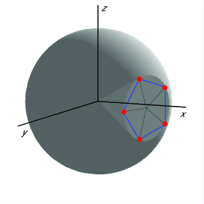
Figure 2: A schematic representation of the circuit’s topology. The critical $x$-axis slices mid-way through an edge that connects two adjacent vertices of the polygon.

As we move along the vertices of the circuit, the critical $x$-axis is crossed in the direction of positive $z$-axis.

VII Results for the Spin-$1/2$ Chain

We now turn to the results of our simulation of the Bargmann invariant for the spin-$1/2$ chain, which are summarized in Fig. 3. The circuit used in the simulation is the regular polygon described in the previous section, but consists of $\mathcal{N}=100$ vertices.

\psfrag{Xlabel}[tc][tc]{}\psfrag{Ylabel}[bc][bc]{}\psfrag{replaceX}[tc][tc]{}\psfrag{replaceY}[bc][bc]{}\includegraphics[width=95.39693pt]{N3cnum100clipped}

\psfrag{Xlabel}[tc][tc]{}\psfrag{Ylabel}[bc][bc]{}\psfrag{replaceX}[tc][tc]{}\psfrag{replaceY}[bc][bc]{}\includegraphics[width=78.70345pt,height=74.88573pt]{N3BargPhaseclipped}

\psfrag{Xlabel}[tc][tc]{}\psfrag{Ylabel}[bc][bc]{}\psfrag{replaceX}[tc][tc]{}\psfrag{replaceY}[bc][bc]{}\includegraphics[width=95.39693pt]{N5cnum100clipped}

\psfrag{Xlabel}[tc][tc]{}\psfrag{Ylabel}[bc][bc]{}\psfrag{replaceX}[tc][tc]{}\psfrag{replaceY}[bc][bc]{}\includegraphics[width=78.70345pt,height=74.88573pt]{N5BargPhaseclipped}

\psfrag{Xlabel}[tc][tc]{}\psfrag{Ylabel}[bc][bc]{}\psfrag{replaceX}[tc][tc]{}\psfrag{replaceY}[bc][bc]{}\includegraphics[width=95.39693pt]{N7cnum100clipped}

\psfrag{Xlabel}[tc][tc]{}\psfrag{Ylabel}[bc][bc]{}\psfrag{replaceX}[tc][tc]{}\psfrag{replaceY}[bc][bc]{}\includegraphics[width=78.70345pt,height=74.88573pt]{N7BargPhaseclipped}

\psfrag{Xlabel}[tc][tc]{}\psfrag{Ylabel}[bc][bc]{}\psfrag{replaceX}[tc][tc]{}\psfrag{replaceY}[bc][bc]{}\includegraphics[width=95.39693pt]{N9cnumclipped}

\psfrag{Xlabel}[tc][tc]{}\psfrag{Ylabel}[bc][bc]{}\psfrag{replaceX}[tc][tc]{}\psfrag{replaceY}[bc][bc]{}\includegraphics[width=78.70345pt,height=74.88573pt]{N9BargPhaseclipped}

\psfrag{Xlabel}[tc][tc]{}\psfrag{Ylabel}[bc][bc]{}\psfrag{replaceX}[tc][tc]{}\psfrag{replaceY}[bc][bc]{}\includegraphics[width=95.39693pt]{11N100cnumclipped}

\psfrag{Xlabel}[tc][tc]{}\psfrag{Ylabel}[bc][bc]{}\psfrag{replaceX}[tc][tc]{}\psfrag{replaceY}[bc][bc]{}\includegraphics[width=78.70345pt,height=74.88573pt]{11N100BargPhaseclipped}

Figure 3: Bargmann invariants and their phases. The rows correspond to the number of spin-$\frac{1}{2}$ particles $N$, increasing from the top as $3,5,7,9,11$. The left column depicts the Bargmann invariants $\mathcal{C}$ on the unit disk in the complex plane, each point of the graph stemming from a different value of the coupling parameter $J$. The right-hand column shows the corresponding Bargmann phase $\varphi/\pi$ as a function of the coupling parameter $(J-J_{c})/r$. See the text for a detailed description of observations.

The Bargmann invariant and its phase were computed for different spin chain lengths, ranging in odd numbers from $3$ to $11$, and shown in Fig. 3 as increasing from the top. Note that the results for even numbers of spins have been omitted as they showed no qualitative difference. This may be due to finite-size effects of the kind which have been observed in similar studies elsewhere, see for example Ref. Kay . The left-hand column of the figure depicts the Bargmann invariants $\mathcal{C}$ on the unit disk in the complex plane. Each data point of the graph stems from a different value of the coupling parameter $J$. The right-hand column shows the corresponding Bargmann phase $\varphi/\pi$, as a function of the coupling parameter $(J-J_{c})/r$, where $r$ refers to the radius of the circle within which the $\mathcal{N}$-polygon circuit is inscribed. Note that in this case the radius was chosen as $10^{-5}$, but the graphs, as they are plotted, are qualitatively independent of the size of this radius.

We would like to point out several features that are apparent from Fig. 3. First and foremost, the Bargmann invariant $\mathcal{C}$ is observed to always pass through the origin of the complex plane just when the spin coupling strength attains its critical value of $J_{c}=1/2$. In other words, the magnitude $|\mathcal{C}|$ vanishes at the critical point. This is one of the features which we would like to propose as a signature of criticality, and is discussed further in section VIII.1.

Another trend that is immediately apparent from Fig. 3 is that with increasing spin chain length the Bargamann invariants ‘wind ever more loops’ around the origin. This statement can be made a little more precise by referring to the corresponding Bargmann phases. These graphs are characterized by discontinuities at the critical point: ‘jumps’ by $\pi$ alternating with ‘jumps’ by $2\pi$. However, on joining up those separate pieces in the graphs end-to-end, one notices that the ‘image’ covered by the resulting graphs grows with $N$ as $\pi(N-1)/2$. This result may be explained by way of referring to the $J=0$ limit of non-interacting spins for which the Berry phase grows linearly with the number of spins. Also note that for spin-$1$ chains, the ‘joined-up’ Bargmann phase covers twice as much ground for any given number of particles (see Fig. 7).

In addition, we should note that we obtain Berry’s solid angle result for the case of non-interacting spins, $J=0$. Approximating the solid angle of our regular polygon circuit as that of the enveloping cone, the Bargmann phase $\varphi$ asymptotically approaches Berry’s solid angle result as the number of vertices of the polygon is increased.

Of course, in the present work only spin chains of up to $11$ particles were simulated, and the exponential growth in the size of the Hilbert space with increasing particle number precludes one from simulating chains that are much longer than that footnote2 . However, from the preceding discussion the trend for Bargmann invariants and phases of longer spin chains should by now be fairly obvious. In particular, it has become clear that, perhaps surprisingly, precious little may be deduced about criticality from the Bargmann phase. Instead, a much clearer indication of the existence of a critical point is the vanishing magnitude of the Bargmann invariant itself.

VIII Signatures of Criticality

VIII.1 Magnitude of the Bargmann Invariant

It was already apparent from Fig. 3 that the magnitude of the Bargmann invariant $\mathcal{C}$ is able to assume the role of a diagnostic tool for critical points in the finite-sized interacting spin chain considered. For clarity, the magnitude of the graphs of $\mathcal{C}$ in Fig. 3 are plotted separately in Fig. 4.

\psfrag{Xlabel}[tc][tc]{$(J-J_{c})/r$}\psfrag{Ylabel}[bc][bc]{$|\mathcal{C}|$}\includegraphics[width=195.12767pt,height=130.08731pt]{abscnum100all}

Figure 4: Plots of $|\mathcal{C}|$ for varying lengths of the spin chain, ranging from $N=3$ to $N=11$ (odd numbers only). The longer the spin chain, the more sharply peaked is the graph. The number of vertices on the circuit is kept constant, at $\mathcal{N}=100$.

An analogous plot is shown in Fig. 5, but this time for a fixed number of spins $N$ and a varying number of circuit vertices $\mathcal{N}$.

\psfrag{Xlabel}[tc][tc]{$(J-J_{c})/r$}\psfrag{Ylabel}[bc][bc]{$|\mathcal{C}|$}\psfrag{a}[tl][tl]{$\mathcal{N}=300$}\psfrag{b}[tl][tl]{$\mathcal{N}=100$}\includegraphics[width=195.12767pt,height=130.08731pt]{N3allabscnumA}

Figure 5: Plots of $|\mathcal{C}|$ for varying numbers of vertices on the circuit, ranging from $\mathcal{N}=100$ to $\mathcal{N}=300$ (in steps of $50$). The more vertices there are on the circuit, the more sharply peaked is the graph. The spin chain length is kept constant, at just $N=3$. Note that qualitatively nothing changes as we increase the chain length (tested up to $N=13$).

Of course, there is a perfectly plausible explanation for these results: as the circuit passes over the critical point the ground state changes abruptly, so that the overlap of the ground states on either side of the critical point will be rather small in magnitude. This in turn forces the magnitude of the product of overlaps along the circuit in Eq. 2 to be small. In fact, similar results were observed in a work by Zanardi and Paunkovi$\acute{\text{c}}$ Zanardi , who concluded that the ground state overlap function is itself a good characterization of QPTs.

VIII.2 ‘Speed’ of the Bargmann Invariant

Another characteristic that is sensitive to the phase transition is the ‘speed’ with which the Bargmann invariant changes as a function of the coupling parameter, which we define by $v_{s}:=|\mathcal{C}_{s+1}-\mathcal{C}_{s}|/(J_{s+1}-J_{s})$. As is evident from Fig. 6, the speed picks up markedly in the vicinity of the critical point. Again, this phenomenon is a direct result of the rapid change of the ground state near a critical point.

\psfrag{Xlabel}[tc][tc]{$(J-J_{c})/r$}\psfrag{Ylabel}[bc][bc]{\text{`speed'} $v$}\includegraphics[width=195.12767pt,height=130.08731pt]{3N100speed}

Figure 6: Plot of the ‘speed’, $v_{s}:=|\mathcal{C}_{s+1}-\mathcal{C}_{s}|/(J_{s+1}-J_{s})$, as a function of the spin coupling strength. The spin chain length is $N=3$ and the circuit is composed of $\mathcal{N}=100$ vertices.

IX Results for the Spin-$1$ Chain

The results presented in Fig. 7 derive from simulations that are entirely analogous to those that gave rise to Fig. 3, but they refer to the spin-$1$ chain model, rather than the spin-$1/2$ model, Eq. 3.

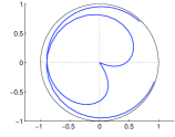
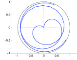
\psfrag{Xlabel}[tc][tc]{$(J-J_{c})/r$}\psfrag{Ylabel}[bc][bc]{$\varphi/\pi$}\includegraphics[width=78.70345pt,height=74.88573pt]{spinone5N100ppclipped}

\psfrag{Xlabel}[tc][tc]{$(J-J_{c})/r$}\psfrag{Ylabel}[bc][bc]{$\varphi/\pi$}\includegraphics[width=78.70345pt,height=74.88573pt]{spinone7N100ppclipped}

\psfrag{Xlabel}[tc][tc]{$(J-J_{c})/r$}\psfrag{Ylabel}[bc][bc]{$\varphi/\pi$}\includegraphics[width=86.72267pt,height=78.04842pt]{spinone5N100ppcontclipped}

\psfrag{Xlabel}[tc][tc]{$(J-J_{c})/r$}\psfrag{Ylabel}[bc][bc]{$\varphi/\pi$}\includegraphics[width=86.72267pt,height=78.04842pt]{spinone7N100ppcontclipped}

\psfrag{Xlabel}[tc][tc]{$(J-J_{c})/r$}\psfrag{Ylabel}[bc][bc]{$\varphi/\pi$}\psfrag{Ylabel}[bc][bc]{$|\mathcal{C}|$}\includegraphics[width=78.04842pt,height=73.7146pt]{spinone5N100abscnumclipped}

\psfrag{Xlabel}[tc][tc]{$(J-J_{c})/r$}\psfrag{Ylabel}[bc][bc]{$\varphi/\pi$}\psfrag{Ylabel}[bc][bc]{$|\mathcal{C}|$}\includegraphics[width=78.04842pt,height=73.7146pt]{spinone7N100abscnumclipped}

Figure 7: These plots depict the Bargmann invariants for spin-$1$ chains of lengths $N=5$ (left-hand column) and $N=7$ (right-hand column), and allow for direct comparison and contrast with the spin-$1/2$ case of Fig. 3. For a detailed description of the results the reader is kindly referred to the text in section IX.

The Bargmann invariants are shown for spin-$1$ chains of lengths $N=5$ (left-hand column) and $N=7$ (right-hand column), and allow for direct comparison and contrast with the spin-$1/2$ case of Fig. 3. The circuit is composed of $\mathcal{N}=100$ vertices. Again, the uppermost row shows the trajectory traced out in the complex plane by the Bargmann invariant as the spin coupling strength is varied from $J_{c}-2r$ to $J_{c}+2r$. The second row from the top shows the corresponding Bargmann phase; notice that points in the immediate vicinity of the critical point have been disregarded as the phase of a complex number becomes increasingly prone to error as the origin of the complex plane is approached. The next row pictures the overall ‘extent’ of the phase, with the individual pieces of the graph having been joined up end-to-end, as described in section VII. Finally, the magnitude of the Bargmann invariant is shown, and is clearly seen to vanish in the vicinity of the critical point.

Qualitatively, the results for spin-$1$ chains are very similar to those of spin-$1/2$ chains. In particular, the magnitude of the Bargmann invariant still represents a signature for the critical point. Of note is also the fact that the ‘joined-up’ Bargmann phase extends twice as high for spin-$1$ chains as it does for spin-$1/2$ chains, for the same number of particles. Again, this can be understood from Berry’s solid angle result for non-interacting particles, where the geometric phase is proportional to the spin dimension.

X Summary and Discussion

In summary, we have shown how the magnitude and ‘speed’ of the Bargmann invariant can act as a signature of the critical point for the finite one-dimensional spin chain model considered. This stands in stark contrast to the Bargmann phase, which is oblivious to the phase transition as long as the spin chain length remains finite.

It is conjectured that the signatures presented here in the context of a specific spin chain model will uphold their validity also in a wider, more general setting. It would be worthwhile to conduct experimental investigations with a view to testing this conjecture; similarly, any theoretical proof of the proposed conjecture would be of considerable interest.

Finally, it is worth stressing that the observed signatures of criticality are very likely a direct consequence of the finite ‘speed’ with which the circuit is traversed in parameter space, i.e. a result of the discrete nature of the circuit. No matter how finely spaced are the neighbouring vertices on the circuit, the adiabatic approximation will always break down in the immediate vicinity of the critical point, causing Landau-Zener tunnelling effects LandauZener to take centre stage. In the limit of a smooth, continuous circuit, the observed signatures of criticality would likely disappear altogether.

- (1) M. Vojta, Rep. Prog. Phys. 66, 2069 (2003).
- (2) M.B. Plenio and S. Virmani, Quant. Inf. Comp. 7, 1 (2007).
- (3) A. Osterloh , L. Amico, G. Falci and R. Fazio, Nature 416 (2002) 608.
- (4) K. Audenaert, J. Eisert, M.B. Plenio and R.F. Werner, Phys. Rev. A 66, 042327 (2002); M.B. Plenio, J. Eisert, J. Dreißig and M. Cramer, Phys. Rev. Lett. 94, 060503 (2005); M. Cramer, J. Eisert, M.B. Plenio and J. Dreißig, Phys. Rev. A 73, 012309 (2006).
- (5) G. Vidal, J. Latorre, E. Rico and A. Kitaev, Phys. Rev. Lett. 90, 227902 (2003).
- (6) J.P. Keating and F. Mezzadri, Commun. Math. Phys. 252, 543 (2004).
- (7) D. Bruss, N. Datta, A. Ekert, L.C. Kwek and C. Macchiavello, Phys. Rev. A 72, 014301 (2005).
- (8) G. Costantini, P. Facchi, G. Florio and S. Pascazio, quant-ph/0612098 (2006).
- (9) V. Vedral, M.B. Plenio, M.A. Rippin and P.L. Knight, Phys. Rev. Lett. 78, 2275 (1997); V. Vedral, M.B. Plenio, K. Jacobs and P.L. Knight, Phys. Rev. A 56, 4452 (1997); V. Vedral and M.B. Plenio, Phys. Rev. A 57, 1619 (1998)
- (10) T.-C. Wei and P.M. Goldbart, Phys. Rev. A 68, 042307 (2003); T.-C. Wei, M. Ericsson, P.M. Goldbart and W.J. Munro, Quant. Inf. Comp. 4, 252 (2004).
- (11) P. Zanardi and N. Paunkovi, Phys. Rev. E 74, 031123 (2006).
- (12) M.V. Berry, Proc. R. Soc. London, Ser. A 392, 45 (1984).
- (13) A. Carollo and J.K. Pachos, Phys. Rev. Lett. 95, 157203 (2005).
- (14) A. Carollo and J.K. Pachos, quant-ph/0602154.
- (15) A. Hamma, quant-ph/060209.
- (16) R. Resta, J. Phys.: Condensed Matter 12 (2000).
- (17) B. Simon, Phys. Rev. Lett. 51, 2167-2170 (1983).
- (18) V. Bargmann, J. Math. Phys. 5, 862 (1964).
- (19) S. Pancharatnam, Proc. Indian Acad. Sci. 44, Sec. A, 247 (1956).
- (20) As an aside, we remark that we only became aware of the vanishing energy gap at in this system as a direct result of observing a discontinuity in the magnitude of the Bargmann invariant. Of course, this is very much in the spirit of this investigation, where Bargmann invariants are assumed to take on a diagnostic role for critical points, even if in hindsight the existence of that critical point is easily demonstrated analytically.
- (21) A. Kay , D.K.K. Lee, J.K. Pachos, M.B. Plenio, M.E. Reuter and E. Rico, Opt. Spectrosc. 99, 339 (2005).
- (22) We note in passing that we have also developed matrix product state algorithms in an attempt to boost the number of particles we can simulate. However, these analyses have not succeded in producing qualitatively new results, over and obove those presented here.
- (23) L.D. Landau, Phys. Z. Sowjetunion 2, 46 (1932); C. Zener, Proc. R. Soc. London, Ser. A 137, 696 (1932).