Dynamics of Josephson-junction qubits with exactly solvable time-dependent bias pulses

Аннотация

The quantum dynamics of a two-state system (qubit) can be governed by means of external control parameters present in time-dependent bias pulses of special forms. We consider the class of biases for which the time evolution equation without a dissipation can be solved exactly. Concentrating for definiteness on the flux qubit we calculate the probability of the definite direction of the current in the loop and its time-averaged values as functions of the qubit’s control parameters both analytically and solving numerically the equation of motion for the density matrix in the presence of relaxation and decoherence. It is shown that there exist such time-dependent biases that the definite current direction probability with no dissipation taken into account becomes a monotonously growing function of time tending to a value which may exceed 1/2. We also calculate the probability to find the system in the excited state and show the possibility of the inverse population in a properly driven two-state system provided the relaxation and dephasing rates are small enough.

I Introduction

In the past few years Josephson junctions-based devices have been widely studied both theoretically and experimentally as possible candidates for the implementation of a quantum computer FromEPJB34(269)1 -FromEPJB34(269)9 . In fact, under appropriate values of external bias pulses, they behave as two-state systems which can be used as a model for quantum bits (qubits). Several systems like ion traps and NMR systems FromEPJB34(269)10 , FromEPJB34(269)11 have been suggested for physical realizations of the qubit but Josephson devices being scalable up to large numbers of qubits as nanocomponents embedded into an electronic circuit exhibit the main technological advantage. Moreover, it is possible to prepare these devices in a prefixed initial state or in a superposition of states and to control their dynamics by an external voltage and magnetic flux FromEPJB34(269)12 .

One common approach to control the qubit dynamics is to drive the two-state system, i.e. a particle in a double well potential, with an oscillating field. As a result an interesting phenomenon may take place. Instead of oscillating between the wells the particle may become localized in one of them. Such an unusual behavior of the quantum particle is known in the literature as coherent destruction of tunneling in double-well potential studies Grossmann67 -Gomes , dynamic localization in transport analysis Raghavan , Dunlap and population trapping in laser-atom physics Agarwal . It is worth stressing that up to now the phenomenon was essentially related with an oscillating character of the driving external field.

In the present article we show that the oscillating character of the field is not compulsory for appearance of the phenomenon. We present a class of non-periodical time-dependent bias pulses leading to a similar behavior of the qubit.

A qubit in the two-state approximation can be described (see e.g. FromEPJB34(269)12 , Reviews ) by the Schrödinger equation

$$i\frac{\partial\Psi}{\partial t}=H\Psi$$

with the Hamiltonian

$$H=\Delta\sigma_{x}+\varepsilon\left(t\right)\sigma_{z}\,,\quad\hbar=1$$ (1)

written down in the basis of “physical” states $\{\left|0\right\rangle,\left|1\right\rangle\}$, which are the eigenstates of the Pauli matrix $\sigma_{z}$ ($\sigma_{z}\left|0\right\rangle=\left|0\right\rangle$, $\sigma_{z}\left|1\right\rangle=-\left|1\right\rangle$) and $\Psi=\left(\psi_{1},\psi_{2}\right)^{T}$. In the case of a charge qubit FromEPJB34(269)1 , these states correspond to a definite number of Cooper pairs on the island (Cooper-pair box). For a flux qubit fluxQbit , they correspond to a definite direction of the current circulating in the ring. In this paper we assume that the tunnelling amplitude $\Delta$ is constant and the bias $\varepsilon$ is a time-dependent function, $\varepsilon=\varepsilon(t)$. Bias $\varepsilon(t)$ is governed by gate voltage $V_{g}(t)$ of the gate electrode close to the Cooper-pair box in the case of a charge qubit and by magnetic flux $\Phi_{x}(t)$ piercing the qubit’s loop in the case of a flux qubit.

For definiteness we will consider here flux qubits. Then “physical” states $\{\left|0\right\rangle,\left|1\right\rangle\}$ are the states with the definite (clockwise or counter-clockwise) direction of the current in the loop. The above mentioned time-dependent biases are, in fact, potentials for which Schrödinger equation (1) can be solved exactly Shamshutdinova -Bagrov . Thus, the probability calculated using these exact solutions is, for example, probability $P^{\uparrow}$ of clockwise current direction. We demonstrate that for some special non-periodical forms of potentials the probability of the clockwise current direction at the moment $t$, if at $t=0$ it was counter-clockwise, becomes a monotonously growing function of time tending to 3/4. Of course this is a strictly fixed excitation regime but we also study the behavior of the probability under small deviations from this specific regime. It should be noted that when parameters of the model are close enough to their specific values, the probability oscillates but its minimal value may exceed 1/2. It is established that such an unusual behavior of the probability is possible even in the presence of a dissipation. We study not only the time evolution of the probability, but also its time-averaged value. Moreover, we also calculate the probability of finding the system in the excited state and show the possibility of the inverse population in the two-state system even in the presence of a dissipation. Our main result is that using a properly chosen non-periodical time-dependent potentials one can ‘‘freeze’’ the qubit state i.e. localize only one of the two possible qubit states for a long time interval. We note that the probability of the definite current flow (or equivalently, the definite magnetic moment of the qubit) is related directly to experimentally measurable values such as the phase shift of the resonant circuit, weakly coupled to the qubit (as discussed, e.g., in Ref. KOSh06 ). Moreover, this “physical” basis is usually used in quantum computations. Thus, we hope that our results offer new opportunities for controlling the qubit behavior. Additional discussion about controlling the level population can be found in Refs. Siewert -Liu .

II Exactly solvable bias pulses

In order to construct an exact solution of a differential equation the intertwining operator technique sometimes may be useful. The idea of the method dates from Darboux papers Darb and is widely used in the soliton theory Matv . Its quantum mechanical application (see e.g. BS ) is related to the fact the one-dimensional stationary Schrödinger equation is an ordinary second order differential equation defined by the operator of the potential energy. The method is based on the possibility to find an operator (intertwining operator) that relates solutions of two Schrödinger equations with different potentials. Thus, if one knows solutions of the Schrödinger equation with a given potential and an intertwining operator is available, there exists a possibility to construct solutions of the same equation with another potential, which cannot be completely arbitrary but is an internal characteristic of the method. There exists also a matrix-differential formulation of the method Matv which was adapted to quantum mechanical problems in Ref. Nieto .

In Shamshutdinova it was shown how to construct differential-matrix intertwining operators for the system of two differential equations of type (1). For that authors Shamshutdinova first reduce system (1) to the one-dimensional stationary Dirac equation with an effective non-Hermitian Hamiltonian where the time plays the role of a space variable and then apply the known procedure developed in Nieto . Starting from the simplest case corresponding to $\varepsilon=\varepsilon_{0}=\mbox{const}$, a new kind of nontrivial potentials (biases) for which Schrödinger equation (1) can be solved exactly were found. Here we apply results obtained in Shamshutdinova -Bagrov to describe the time evolution of the qubit, time dependence of the qubit localization probability and calculate its time-averaged value.

Consider first the case when bias $\varepsilon=\varepsilon(t)$ changes in the following way:

$$\varepsilon_{1}\left(t\right)=\varepsilon_{0}-\frac{4\varepsilon_{0}}{1+4\varepsilon_{0}^{2}t^{2}}\;.$$ (2)

In Ref. Shamshutdinova a detailed analysis of solutions to equation (1) in this case is given. Therefore imposing the initial conditions $|\psi_{1}\left(0\right)|^{2}=1$ and $|\psi_{2}\left(0\right)|^{2}=0$ one finds probability $P^{\uparrow}\left(t\right)=|\psi_{2}\left(t\right)|^{2}$ of, for example, the clockwise current direction at the moment $t$ if at $t=0$ it was counter-clockwise. For $\tau=\Delta t$ and $\xi=\frac{\varepsilon_{0}}{\Delta}$ it reads

$$P_{1}^{\uparrow}\left(\tau\right)=\frac{1}{\Theta^{6}\left(1+4\xi^{2}\tau^{2}\right)}\times\\ \left[16\xi^{4}\Theta^{2}\tau^{2}\cos^{2}\Theta\tau+4\xi^{2}\Theta\tau\left(1-3\xi^{2}\right)\sin 2\Theta\tau+\left(4\xi^{2}\Theta^{4}\tau^{2}+\left(1-3\xi^{2}\right)^{2}\right)\sin^{2}\Theta\tau\right],$$ (3)

$$\Theta=\sqrt{1+\xi^{2}}\;.$$

It is clearly seen from here that $P_{1}^{\uparrow}(\tau)$ is an oscillating function provided $\xi^{2}\neq\frac{1}{3}$. For $\xi^{2}=\frac{1}{3}$ the probability becomes equal

$$P_{1}^{\uparrow}\left(\tau\right)=\frac{\tau^{2}}{1+\frac{4}{3}\tau^{2}}\;,$$ (4)

which is a function monotonically growing from zero at the initial time moment till the value $3/4$ at $\tau\gg 1$ or $t\gg\Delta^{-1}$ (see the thick line in Fig. 1a). It is important to note that at $\xi^{2}$ close enough to $\frac{1}{3}$ the value of probability $P_{1}^{\uparrow}$ exceeds $1/2$ very quickly (see the thin and dotted lines in Fig. 1a).

For the time-averaged probability one gets

$$\overline{P_{1}^{\uparrow}}=\frac{1+5\xi^{2}}{2\left(1+\xi^{2}\right)^{2}}\;.$$ (5)

It follows from Eq. (5) that at $\xi^{2}=\frac{3}{5}$ the averaged probability exhibits a kind of the resonance behavior, i.e. it peaks to its maximal value $\overline{P_{1}^{\uparrow}}\approx 0.78$, (see the thick line in Fig. 2) although for any given $\xi$ $P_{1}^{\uparrow}\left(\tau\right)$ is a function asymptotically oscillating with frequency $4\sqrt{\frac{2}{5}}$ (see Fig. 1).

More exactly solvable potentials may be obtained with the help of chains of the above simple transformations. Ref. PolPSUSY contains a detailed analysis of the properties of such chains. The authors show how to generate a large family of new exactly solvable biases for equation (1). For a two-fold transformation leading to the bias of the form

$$\varepsilon_{2}\left(t\right)=\frac{\varepsilon_{0}\left(45-180\varepsilon_{0}^{2}t^{2}-144\varepsilon_{0}^{4}t^{4}+64\varepsilon_{0}^{6}t^{6}\right)}{9+108\varepsilon_{0}^{2}t^{2}+48\varepsilon_{0}^{4}t^{4}+64\varepsilon_{0}^{6}t^{6}}$$ (6)

the clockwise current direction probability is given by

$$P_{2}^{\uparrow}\left(\tau\right) = \frac{1}{\Theta^{10}\left(9+108\xi^{2}\tau^{2}+48\xi^{4}\tau^{4}+64\xi^{6}\tau^{6}\right)}$$ (7)

$$\times \biggl{(}16\xi^{4}\Theta^{2}\tau^{2}\left[16\xi^{4}\Theta^{4}\tau^{4}+24\xi^{2}\left(3-14\xi^{2}+7\xi^{4}\right)\tau^{2}+9\left(9-6\xi^{2}+\xi^{4}\right)\right]$$

$$+ Q_{1}\left[Q_{2}\sin^{2}\Theta\tau+Q_{3}\sin 2\Theta\tau\right]\biggr{)}$$

where

$$\begin{array}[]{l}Q_{1}=1-10\xi^{2}+5\xi^{4}\,,\\ Q_{2}=64\xi^{6}\Theta^{4}\tau^{6}+48\xi^{4}\left(1-18\xi^{2}-19\xi^{4}\right)\tau^{4}+36\xi^{2}\left(3-2\xi^{2}+11\xi^{4}\right)\tau^{2}+9Q_{1}\,,\\ Q_{3}=12\xi^{2}\Theta\tau\left(\Theta^{2}\left(16\xi^{4}\tau^{4}+7\right)+2\left(4\xi^{2}\tau^{2}+1\right)\left(1-5\xi^{2}\right)\right).\end{array}$$

The last term in Eq. (7) describes the oscillations with frequency $2\Theta$ and, hence, under the condition $Q_{1}=0$ the oscillations in the time-dependence of the probability disappear and it acquires a monotonous character. Therefore, for $\varepsilon$ as given in (6), unlike (2), we can indicate two possibilities for $Q_{1}=0$. So, the probability of the clockwise current direction turns from an oscillating to a monotonous function of time both at $\xi=\sqrt{1-2/\sqrt{5}}$ and $\xi=\sqrt{1+2/\sqrt{5}}$. This behavior is illustrated in Fig. 1b (thick lines) where we also show an oscillating character of the probability for the parameter $\xi$ close to the above critical values (thin and dotted lines).

Time-averaged probability (7) for $\varepsilon\left(t\right)$ of the form (6) is given by

$$\overline{P_{2}^{\uparrow}}=\frac{1-2\xi^{2}+13\xi^{4}}{2\left(1+\xi^{2}\right)^{3}}\,.$$ (8)

The $\xi$-dependence of $\overline{P_{2}^{\uparrow}}$ is demonstrated in Fig. 2b by the thick line. It has a maximum $\overline{P_{2}^{\uparrow}}\approx 0.91$, at $\xi\approx 1.46$.

Let us consider a more complicated case Shamshutdinova , Bagrov when the bias contains three free parameters

$$\varepsilon_{3}\left(t\right)=\varepsilon_{0}+\frac{2\omega^{2}}{b\cos\left(2\omega t+\varphi\right)-\varepsilon_{0}}\;,\quad b^{2}=\varepsilon_{0}^{2}-\omega^{2}>0\,.$$ (9)

Here $\varphi$ is arbitrary but $\varepsilon_{0}$ and $\omega$ should satisfy the inequality given in Eq. (9). We note that in this case $\varepsilon=\varepsilon_{3}(t)$ is a periodical function with an amplitude related with frequency. Expression (9) presents a generalization of formula (2). Indeed, putting $\varphi=\arctan\frac{\omega}{2\varepsilon_{0}}-\frac{1}{2}\arctan\frac{\omega}{b}$ in Eq. (9), in the limit $\omega\rightarrow 0$ one recovers for $\varepsilon$ result (2).

The analytic expression for $P_{3}^{\uparrow}(\tau)$ is rather involved and we will restrict ourselves to a graphical illustration of the clockwise current direction probability at $\Theta\approx\frac{\omega}{\Delta}$, (see Fig. 3). More graphical illustrations can be found in Shamshutdinova .

III Influence of a dissipation on probabilities

A quantum system described by a wave function which is a solution of the Schrödinger equation with Hamiltonian (1) interacts only with an external field described by function $\varepsilon(t)$. But in real experiments there is also an interaction of a Josephson junction device with an external reservoir which makes impossible describing the system in terms of a wave function since its state is not a pure quantum state anymore and should be described withe the help of a density matrix (operator in general see e. g Breuer ) formalism. Such kind of systems are particularly important in the context of quantum information processing where environment-induced decoherence is viewed as a fundamental obstacle for constructing a quantum information processors (e.g., Lidar ).

In this section we study the behavior of the qubit with bias $\varepsilon(t)$ as given in Eqs. (2), (6) and (9) taking into account the dephasing and the relaxation processes. We also study a possibility of the inverse population in the two-level system and investigate how it is influenced by a decoherence. It is worth noticing that in contrast to Ref. Siewert , where the authors investigate a three-level system, we study a possibility of the inverse population for the two level system itself thus showing the possibility of building a two-level based laser working at a low temperature.

To study the dynamic behaviour of the qubit, we use the master equation for the density matrix. For the density matrix of the form

$$\widehat{\rho}=\frac{1}{2}\left[\begin{array}[]{cc}1+Z&X-iY\\ X+iY&1-Z\end{array}\right]$$

we solve the equation of motion

$$i\frac{\partial\widehat{\rho}}{\partial t}=[\widehat{H}\widehat{\rho}]$$

to obtain the probability $P^{\uparrow}=[1-Z(t)]/2$. The effect of the relaxation processes on the system due to a weak coupling to the environment can be phenomenologically described by two parameters, the dephasing ($\Gamma_{\varphi}$) and relaxation ($\Gamma_{relax}$) rates (see e.g. Ref. ShKOK ), which we introduce phenomenologically thus obtaining the following system of equations for $X(t)$, $Y(t)$ and $Z(t)$:

$$\frac{dX}{dt} =-2\varepsilon(t)Y-\Gamma_{\varphi}X,$$

$$\frac{dY}{dt} =-2\Delta Z+2\varepsilon(t)X-\Gamma_{\varphi}Y,$$

$$\frac{dZ}{dt} =2\Delta Y-\Gamma_{relax}\left(Z-Z(0)\right).$$

In order to verify the possibility of the inverse population in the two-level system we also calculate the probability $P^{+}$ ShKOK of finding the system on the upper level (excited state).

To see the influence of the relaxation on probabilities $P_{1}^{\uparrow}$ and $P_{1}^{+}$ exhibiting a monotonous time dependence for $\varepsilon(t)$ in form (2) we choose $\xi=1/\sqrt{3}$ and plot them in Fig. 4. We do not show the behavior of $P_{2}^{\uparrow}$ and $P_{2}^{+}$ corresponding to $\varepsilon(t)$ as given in (6) since it is similar to that displayed in Fig. 4. Fig. 5 illustrates the evolution of probabilities $P_{3}^{\uparrow}(t)$ and $P_{3}^{+}$ when $\varepsilon(t)$ has form (9) with $\xi=\frac{1}{\sqrt{3}}$, $\beta=\frac{\sqrt{15}}{2}$, $\varphi=0$. Thick lines on these figures correspond to $\Gamma_{\varphi}=\Gamma_{relax}=0$ when no relaxation is present in the system. Thin and dotted lines just show the relaxation effect for $\Gamma_{\varphi}=\Gamma_{relax}=0.01$ and $\Gamma_{\varphi}=\Gamma_{relax}=0.1$ respectively. All values are in units of $\Delta$. It is clearly seen from here that the inverse population is still possible even if the dissipation is present but during a small time interval $\tau$ only.

Time-averaged probabilities $\overline{P_{1}^{\uparrow}}$ and $\overline{P_{2}^{\uparrow}}$ are plotted in Fig. 2a and 2b as functions of dimensionless parameter $\xi$. Here the thick lines also correspond to the absence of the relaxation and the thin and dotted lines illustrate the relaxation effect for the same values of $\Gamma_{\varphi}=\Gamma_{relax}$ as in Figs. 4 and 5. The dash-dotted curves are drown for $\Gamma_{\varphi}/\Delta=\Gamma_{relax}/\Delta=0.001$. These results show the possibility of the inverse population only for small enough dissipation (see the dash-dotted lines) and for parameter $\xi$ close enough to its critical values when the averaged probabilities pick to their maximal values.

IV Conclusion

In conclusion, a two-state system subjected to biases of special forms, for which the Schrödinger equation is exactly solvable, was considered. For definiteness we studied the time-evolution of the Josephson-junction qubit, but the similar consideration can be applied to other realizations of a two-state system. We have demonstrated that the dynamics of the Josephson-junction qubit displays in these cases several nontrivial features. Varying the form of the time dependent bias, one can change qualitatively the dynamic behavior of the occupation probabilities. In particular, the amplitude of the oscillating probability, describing the definite current direction in the loop, can be tuned to zero, thus turning the probability to a monotonous function of time. We calculate the probability of finding the system in the excited state and show that the inverse population in the two-state system is possible even in the presence of a dissipation. The observation of such an occupation probability behavior may be related to experimentally measurable values, which would make an experimental verification of the theoretical predictions of the present paper.

V.V.S. acknowledges a partial support from INTAS Fellowship Grant for Young Scientists Nr 06-1000016-6264. S.N.S and A.N.O. acknowledge the grant “Nanosystems, nanomaterials, and nanotechnology” of the National Academy of Sciences of Ukraine. The work of S.N.S. was partly supported by grant of President of Ukraine (No. GP/P11/13). The work of B.F.S. is partially supported by grants RFBR-06-02-16719 and SS-5103.2006.2.

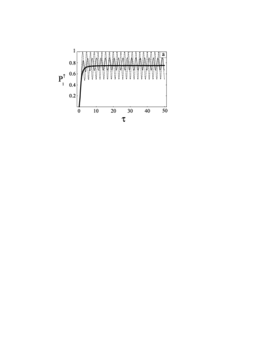
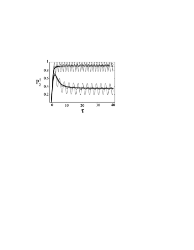
Рис. 1: Time dependence of clockwise current direction probabilities. (a) $P_{1}^{\uparrow}$ probability evolution at $\xi=\sqrt{\frac{1}{2}}$ (thin line), $\xi=1$ (dotted line) and $\xi=\sqrt{\frac{1}{3}}$ (thick line). (b) $P_{2}^{\uparrow}$ probability evolution at $\xi=\sqrt{2+\frac{2}{\sqrt{5}}}$, $\xi=\sqrt{1.2+\frac{2}{\sqrt{5}}}$ and $\xi=\sqrt{1+\frac{2}{\sqrt{5}}}$ on the upper plot, $\xi=\sqrt{1.05-\frac{2}{\sqrt{5}}}$, $\xi=\sqrt{1.01-\frac{2}{\sqrt{5}}}$ and $\xi=\sqrt{1-\frac{2}{\sqrt{5}}}$ on the lower plot (dotted, thin and thick lines respectively).

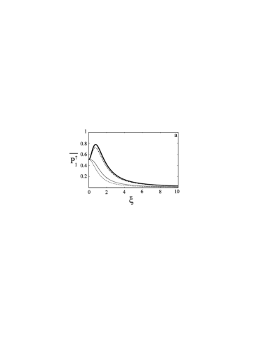
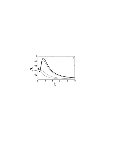
Рис. 2: $\xi$-dependence of time-averaged probabilities.

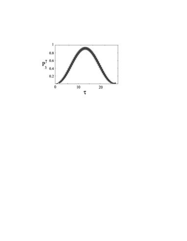
Рис. 3: Time dependence of clockwise current direction probabilities. $P_{3}^{\uparrow}$ probability evolution at $\theta=6.88$, $\Theta=7$, $\xi=\sqrt{48}$, $\varphi=0$.

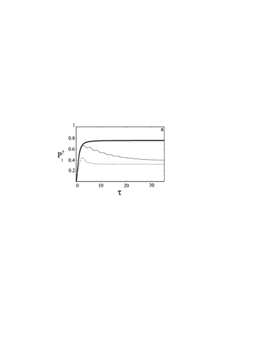
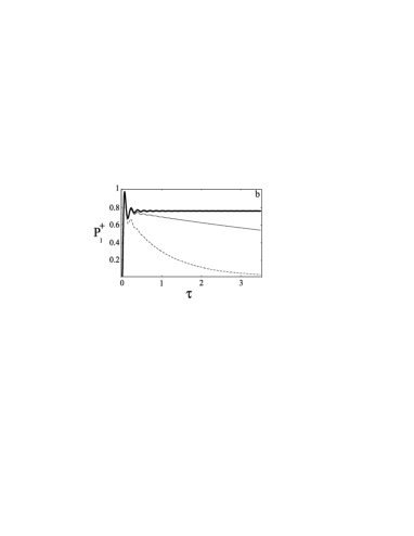
Рис. 4: The influence of relaxation on the probabilities. (a) The clockwise current direction probability $P_{1}^{\uparrow}$ at $\xi=1/\sqrt{3\text{.}}$ (b) The upper level occupation probability $P_{1}^{+}$ at $\xi=1/\sqrt{3\text{.}}$

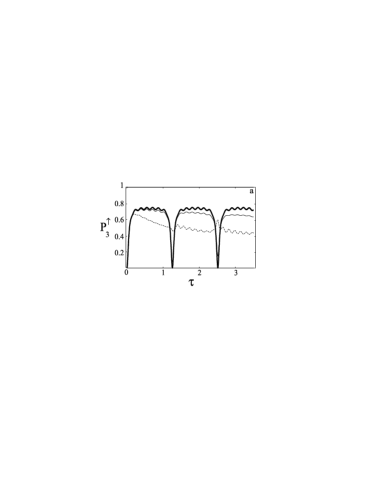
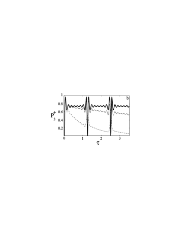
Рис. 5: The influence of relaxation on the probabilities. (a) The clockwise current direction probability $P_{3}^{\uparrow}$ at $\xi=\frac{1}{\sqrt{3}}$, $b=\frac{\sqrt{15}}{2}$, $\varphi=0$. (b) The upper level occupation probability $P_{3}^{+}$ at $\xi=\frac{1}{\sqrt{3}}$, $b=\frac{\sqrt{15}}{2}$, $\varphi=0$.

- (1) Y. Nakamura, Yu. A. Pashkin, and J. S. Tsai, Nature (London) 398, 786 (1999).
- (2) Y. Nakamura, Yu. A. Pashkin, and J. S. Tsai, Phys. Rev. Lett. 87, 246601 (2001).
- (3) D. Vion, A. Aassime, A. Cottet et al., Science 296, 886 (2002).
- (4) Y. Yu, S. Han, X. Chu et al., Science 296, 889 (2002).
- (5) J. M. Martinis, S. Nam, J. Aumentado, and C. Urbina, Phys. Rev. Lett. 89, 117901 (2002).
- (6) Y. Makhlin, G. Schön, and A. Shnirman, Physica C 368, 276 (2002).
- (7) Yu. A. Pashkin, T. Yamamoto, O. Astafiev et al., Nature (London) 421, 823 (2003).
- (8) I. Chiorescu, Y. Nakamura, C. J. Harmans, and J. E. Mooij, Science 299, 1869 (2003).
- (9) A. Blais, A. Maassen van den Brink, and A. M. Zagoskin, Phys. Rev. Lett. 90, 127907 (2003).
- (10) S. Braunstein and H. - K. Lo, Special Focus Issue: Experimental Proposals for Quantum Computers, Fortschr. Phys. 48, No 9-11 (2000).
- (11) R. G. Clark, Experimental Implementation of Quantum Computation, Rinton Press (2001).
- (12) Y. Makhlin, G. Schön, and A. Shnirman, Rev. Mod. Phys. 73, 357 (2001).
- (13) F. Grossmann, T. Dittrich, and P. Hänggi, Phys. Rev. Lett. 67, 516 (1991).
- (14) F. Grossmann, P. Jung, T. Dittrich, and P. Hänggi, Z. Phys. B 85, 315 (1991).
- (15) F. Grossmann and P. Hänggi, Europhys. Lett. 18, 571 (1992).
- (16) J. - M. Lopez-Castillo, A. Filali-Mouhim, and J. - P. Jay-Gerin, J. Chem. Phys. 97, 1905 (1992).
- (17) R. I. Cukier, M. Morillo, and J. M. Casado, Phys. Rev. B 45, 1213 (1992).
- (18) J. M. Gomes Llorente and J. Plata, Phys. Rev. A 45, R6958 (1992).
- (19) S. Raghavan, V. M. Kenkre, D. H. Dunlap et al., Phys. Rev. A 54, R1781 (1996).
- (20) D. H. Dunlap and V. M. Kenkre, Phys. Rev. B 34, 3625 (1986).
- (21) G. S. Agarwal and W. Harshawardhan, Phys. Rev. A 50, R4465 (1994).
- (22) G. Wendin and V. S. Shumeiko, Superconducting circuits, qubits and computing, Handbook of Theoretical and Computational Nanotechnology, ed. by M. Rieth and W. Schommers, American Scientific Publishers (2006), ch. 12; arXiv:cond-mat/0508729.
- (23) J. E. Mooij, T. P. Orlando, L. Levitov et al., Science 285, 1036 (1999).
- (24) B. F. Samsonov, V. V. Shamshutdinova, J. Phys. A 38, 4715 (2005).
- (25) B. F. Samsonov, V. V. Shamshutdinova, and D. M. Gitman, Czech. J. Phys. 55 No 9, 1173 (2005).
- (26) V. V. Shamshutdinova, Boris F. Samsonov, and D. M. Gitman, Ann. Phys. (NY) 2006 (to be published).
- (27) V. G. Bagrov, M. C. Baldiotti, D. M. Gitman, V.V. Shamshutdinova, Ann. Phys. 14 (6) (2005) 390.
- (28) A. S. Kiyko, A. N. Omelyanchouk, and S. N. Shevchenko, submitted in Proceedings of Int’l Symposium on Mesoscopic Superconductivity and Spintronics, Japan (2006).
- (29) J. Siewert, T. Brandes, and G. Falci, arXiv:cond-mat/0509735.
- (30) M. Grifoni and P. Hänggi, Phys. Rep. 304, 229 (1998).
- (31) M. Steffen, J.M. Martinis, and I.L. Chuang, Phys. Rev B 68, 224518 (2003).
- (32) Yu-xi Liu, J. Q. You, L. F. Wei et al., Phys. Rev. Lett. 95, 087001 (2005).
- (33) G. Darboux, Compt. Rend. Acad. Sci. Paris 94, 1343 (1882); Darboux, Compt. Rend. Acad. Sci. Paris 94, 1456 (1882); Darboux, Leçons sur la théorie générale des surfaces et les application géométriques du calcul infinitésimale. Deuxiem partie, Gautier-Villar et Fils, Paris (1889).
- (34) V. Matveev and M. Salle, Darboux transformations and solitons, Springer, New York (1991).
- (35) V. G. Bagrov and B. F. Samsonov, Theor. Math. Phys. 104, 1051 (1995).
- (36) I. M. Nieto, A. A. Pecheritsin, and B. F. Samsonov, Ann. Phys. (NY) 305 No 2, 151 (2003).
- (37) H. - P. Breuer and F. Petruccione, The Theory of Open Quantum Systems, Oxford University Press, Oxford (2002).
- (38) D. A. Lidar and K. B. Whaley, in Irreversible Quantum Dynamics, ed. by F. Benatti and R. Floreanini, Lecture Notes in Physics, Springer, Berlin (2003), Vol. 622, p. 83; arXiv:quant-ph/0301032.
- (39) S. N. Shevchenko, A. S. Kiyko, A. N. Omelyanchouk, and W. Krech, Fiz. Nizk. Temp. 31, 752 (2005); Low Temp. Phys. 31, 564 (2005).