Realization of quantum mechanical weak values of observables using entangled photons

Abstract

We present a scheme for realization of quantum mechanical weak values of observables using entangled photons produced in parametric down conversion. We consider the case when the signal and idler modes are respectively in a coherent state and vacuum. We use a low efficiency detector to detect the photons in the idler mode.This weak detection leads to a large displacement and fluctuations in the signal field’s quantum state which can be studied by monitoring the photon number and quadrature distributions.

In a remarkable paper Aharonov, Albert and Vaidman aharonov discovered that under conditions of very weak coupling between the system and the measuring device the uncertainty in a single measurement could be very large compared with the separation between the eigenvalues of the observable. This is quite a departure from the usual idea of projective measurements where the measurement projects on to one of the eigenvalues VonNeumann . Aharonov et al proposal was further clarified by several authorsduck ; johansen ; knight ; ruseckas . In particular Duck et al. duck also suggested an optical experiment to verify the idea. Such an optical experiment was performed by Ritchie et al. ritchie . This experiment uses the classical light source like a laser beam; a birefringent medium and the pre and post selection of the polarization of the transmitted beam. The experiment is well explained using classical physics as discussed in the paper by Ritchie et al ritchie . It would therefore be interesting to find situations which are strictly quantum in nature even though the experiment of Ritchie et al. was repeated at single photon level and in particular weak values of photon arrival times were measured ahnert . Further weak values of the polarization of a single photon were reported wiaeman2 . In this letter we show how the idea of Aharonov et al could be realized using entangled photons produced in the process of parametric down conversion thus making their proposal within the reach of current experiments. We specifically discuss the weak values associated with the measurement of the photon number and the quadrature of the signal field. We also discuss how the weak values reflect in the fluctuations of the state of the signal field. Our explicit result for the state of the signal field shows the role of quantum interferences in the weak values of the observables. We require two ingredients for the observation-high value of the squeezing parameter and well controlled detector. Both of these are feasible. We note that Zambra et al zambra have very successfully demonstrated the application of avalanche detectors for the reconstruction of photon statistics. Further in recent experiments caminati high values of the squeezing parameter have been achieved. We note [cf Eqs.(9), (10), (15)] that if the squeezing is not very high then we need to use smaller detection efficiencies. Our proposal contrasts the previous ones ritchie ; gisin which used classical Gaussian beams and birefringent medium.

In Fig. 1, we show a schematic arrangement for realization of the weak values using entangled photons. The entangled photons are generated by an optical parametric amplifier (OPA). In OPA the pump field interacts nonlinearly in an optical crystal having second order nonlinearity. As a result of annihilation of one photon of pump field two entangled photons propagating in two different directions are generated simultaneously. In our scheme, we consider that the signal mode is initially in a coherent state $|\alpha\rangle$ while the idler is initially in vacuum. The photons generated in signal mode produce excitation tara in coherent field $|\alpha\rangle$ presented initially. If $n$-photons are generated in the idler mode, the state of the signal mode will be in $n$-photon added coherent state. In our scheme, we perform weak detection of the idler photons by using a low efficiency detector which requires a large number of photons to be produced in the idler mode. Thus we consider OPA working under high gain conditions.

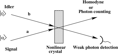
Figure 1: The schematic arrangement for realization of weak values using entangled photons. The idler photon is detected with varying efficiency.

We note that a similar arrangement with OPA under low gain conditions has been used in a recent experiment by Zavatta et al Zavatta , for generating photon added coherent states tara . Using the interaction Hamiltonian for the OPA and under the assumption of no pump depletion, the state of the outgoing signal and idler fields can be written as

$$|\psi\rangle=\exp\left(ra^{{\dagger}}b^{{\dagger}}-rab\right)|\alpha,0\rangle$$ (1)

where $r$ is gain of the amplifier. Using the Baker Campbell Hausdorff identity, the Eqn (1) simplifies to

$$|\psi\rangle = \exp\left(\tanh ra^{{\dagger}}b^{{\dagger}}\right)\exp\left[-\ln\cosh r(a^{{\dagger}}a+b^{{\dagger}}b+1)\right]$$ (2)

$$\times\exp\left(-\tanh rab\right)|\alpha,0\rangle$$

$$= \frac{e^{-\frac{1}{2}|\alpha|^{2}\tanh^{2}r}}{\cosh r}\exp\left(\tanh ra^{{\dagger}}b^{{\dagger}}\right)|\alpha^{\prime},0\rangle$$

where $\alpha^{\prime}=\alpha/\cosh r$. The Eq (2) shows how the OPA generates correlated pair of photons one in signal mode and one in idler mode simultaneously. According to the von Neumann postulate the measurement of the state of the idler mode in $n$-photon Fock state $|n\rangle$ would project the state of the signal mode in $n$-photon added coherent state $a^{{\dagger}n}|\alpha^{\prime}\rangle$. However we now follow the idea of Aharonov et al on weak measurements. We measure idler field weakly, i.e. the measurement does not make the idler field to collapse in a single Fock state, with definite number of photons, but a probabilistic mixture of various Fock states of different number of photons. The weak detection is performed by a low efficiency detector footnote . Clearly, the weak measurement of the idler field will project the signal field in a superposition of various photon added coherent statestara . We would now show how the weak detection of idler photons leads to unexpectedly large values of signal field. The density matrix for signal-idler fields is

$$\rho=|\psi\rangle\langle\psi|,$$ (3)

where $|\psi\rangle$ is given by Eq.(2). We detect idler field in the $n$-photon Fock state $|n\rangle$ by using a detector of quantum efficiency $\eta$. The projected state of the signal field is

$$\rho_{n}^{(s)}=A\sum_{m=n}^{\infty}\left(\begin{array}[]{c}m\\ n\end{array}\right)\eta^{n}(1-\eta)^{n-m}\langle m|\rho|m\rangle,$$ (4)

where $A$ is normalization constant. Using (3) and (2), Eq (4) takes the form

$$\rho_{n}^{(s)}=N\sum_{m=n}^{\infty}\left(\begin{array}[]{c}m\\ n\end{array}\right)\eta^{n}(1-\eta)^{n-m}\frac{\tanh^{2m}r}{m!}a^{{\dagger}m}|\alpha^{\prime}\rangle\langle\alpha^{\prime}|a^{m},$$ (5)

where $N$ is new normalization constant and the constant term $e^{-|\alpha|^{2}\tanh^{2}r}/\cosh^{2}r$ has been absorbed in $N$.

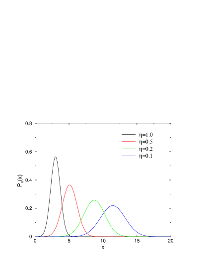
Figure 2: (Color online) The quadrature distribution of signal field after measuring idler photons in vacuum state by using detector of efficiency $\eta$.

From Eq (5), it is clear that because of non-unity quantum efficiency of the detector, the measurement of the idler field can not project the signal field in one of its eigenstate. The projected state of the signal field is a superposition of various eigenstates. Further, for smaller values of $\eta$ and larger values of OPA gain parameter $r$, many eigenstates in the superposition contributes significantly.

It should be noted here, that in our scheme we do not perform measurement on a two state system as discussed by Aharonov et al aharonov in their original proposal. We perform measurement on an infinite dimensional system. Here we are particularly interested in detecting the idler field in vacuum state. Note that the detection of idler in vacuum state for a range of values of the efficiency is enough to reconstruct the full idler field zambra . From Eq.(5), the weak measurement of the idler field in the state $|0\rangle$, projects the signal field in the state

$$\rho_{0}^{(s)}=N\sum_{m=0}^{\infty}(1-\eta)^{m}\frac{\tanh^{2m}r}{m!}a^{{\dagger}m}|\alpha^{\prime}\rangle\langle\alpha^{\prime}|a^{m}.$$ (6)

The above conditional state of the signal field can be measured either through the photon number distribution or via the quadrature distribution.We next calculate these and show how the weak values get reflected in such distributions.

The quadrature distribution of the projected signal field (6), when idler field is detected in the vacuum state by using detector of quantum efficiency $\eta$, is given by

$$P_{0}(x)=N\sum_{m=0}^{\infty}(1-\eta)^{m}\frac{\tanh^{2m}r}{m!}\langle x|a^{{\dagger}m}|\alpha^{\prime}\rangle\langle\alpha^{\prime}|a^{m}|x\rangle,$$ (7)

where $|x\rangle$ is eigenstate in the quadrature space.A long calculation leads to the following compact expression for the quadrature distribution of the signal field

$$P_{0}(x)=\sqrt{\frac{1-\epsilon}{\pi(1+\epsilon)}}\exp\left[-\frac{1-\epsilon}{1+\epsilon}\left(x-\frac{\sqrt{2}\alpha^{\prime}}{1-\epsilon}\right)\right]$$ (8)

where $\epsilon=(1-\eta)\tanh^{2}r$. From Eq (8), it is clear that the projected state of the signal field (6) has Gaussian quadrature distribution. The peak of the distribution appears at

$$x=\sqrt{2}\alpha^{\prime}/(1-\epsilon),$$ (9)

and the width of the distribution $\delta x$ is given by

$$2(\delta x)^{2}=\frac{1+\epsilon}{1-\epsilon}.$$ (10)

It is clear from Eq (9) and Eq (10) that for low efficiency detector $(\eta<<1)$ and high gain OPA $(r>1)$, as the value of $\epsilon$ tends towards $1$, the peak in the quadrature distribution occurs for exceptionally large values of $x$. Further, the width of the distribution also becomes very large for these values of the parameters.Interestingly enough in our model the width of the distribution also depends on the weakness of the measurement.

In Fig.2, we show the quadrature distributions of the projected states of the signal field after detecting the idler field in vacuum state. For 100% detection efficiency the maxima in the quadrature distributions occurs at $x\approx 3$ corresponding to the value $x=\sqrt{2}\alpha^{\prime}$, where $\alpha^{\prime}=\alpha/\cosh r$ and $\alpha=5$ and $r=1.5$. We find that for lower detection efficiency the maxima in the quadrature distribution shifts to the exceptionally larger values of $x$. For $\eta=0.1$ the maxima in x-quadrature appears around $x\approx 12$. Further, the spread in the distribution becomes very large for such smaller values of $\eta$. This is a remarkable realization of the idea of Aharonov et al using entangled photons.

In order to understand the exact nature of the weak values we look at Eq(6) for the projected state of the signal field. Clearly, the projected state of the signal field is superposition of photon added coherent states $a^{{\dagger}m}|\alpha^{\prime}\rangle$ generated by successive addition of the photons in the signal mode. The amplitude of the $m$-th term in Eq(6) is proportional to $\epsilon^{m}/m!$, where $\epsilon=(1-\eta)\tanh^{2}r$. For $\eta=0.1$ and $r=1.5$, as the value of $\epsilon$ is $0.74$, the amplitude of the fifth term is of the order of $10^{-3}$. Further the higher order terms will have much smaller amplitude and can be neglected. The quadrature distribution of $5$-photon added coherent state $a^{{\dagger}5}|\alpha^{\prime}\rangle$ will have maxima at $x\approx\sqrt{2}\sqrt{|\alpha^{\prime}|^{2}+5}$. Thus the highest order contributing eigen state of the signal field has maxima at $x\approx 4.5$. In Fig.3 the maxima in the quadrature distribution corresponding to these parameters occurs at $x\approx 12$, which is exceptionally large and there is no doubt that the projected values of the signal field in our scheme are weak values. The exceptional displacement in the maxima of the quadrature distribution occurs as a result of interferences between various states contributing to the projected state of the signal field. Further it should also be noted that the photon added coherent states $a^{{\dagger}m}|\alpha^{\prime}\rangle$ show more and more squeezing in their quadrature on increasing $m$ tara , while the projected state of the signal field exhibits broadening in the quadrature distribution. Clearly choosing smaller detection efficiencies (few %) which are definitely feasible zambra would lead to larger displacement and large fluctuations.

Next we show how the weak measurements get reflected in the photon number distribution of the signal field.The photon distribution of the projected state of the signal field (6) is calculated as follows

$$P_{0}(n)=N\sum_{m=0}^{\infty}(1-\eta)^{m}\frac{\tanh^{2m}r}{m!}\langle n|a^{{\dagger}m}|\alpha^{\prime}\rangle\langle\alpha^{\prime}|a^{m}|n\rangle,$$ (11)

$$P_{0}(n) = N(1-\eta)^{n}\tanh^{2n}r\times$$ (12)

$$\sum_{m=0}^{n} \frac{n!}{m!(n-m)!^{2}}\left(\frac{\alpha^{\prime 2}}{(1-\eta)\tanh^{2}r}\right)^{n-m}.$$

Using definition of Laguerre polynomials and evaluating the normalization constant, the Eq (12) takes the form

$$P_{0}(n)=(1-\epsilon)e^{-\alpha^{\prime 2}/(1-\epsilon)}\epsilon^{n}L_{n}\left(-\frac{\alpha^{\prime 2}}{\epsilon}\right)$$ (13)

where $L_{n}(q)$ is Laguerre polynomial of order $n$.

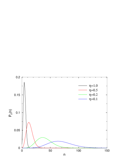
Figure 3: (Color online) The photon distribution of signal field after measuring idler photons by using detector of efficiency $\eta$. The idler field is detected in vacuum state $|0\rangle$

The photon distributions of the projected signal state (6) are shown in Fig.3. For unity detection efficiency the field has maxima at $n\approx 5$ corresponding to the coherent state $|\alpha^{\prime}\rangle$. As the detection efficiency $\eta$ decreases the peak in the distribution moves very fast towards the higher values of $n$ and the width of the distribution also increases. As we have discussed earlier, for $\eta=0.1$, only terms up to $m=5$ can contribute significantly in the projected signal state (6). Thus the signal field contains its highest order eigenstate having maxima in the photon distribution at $|\alpha^{\prime}|^{2}+5\approx 10$. But the actual weak value of the maximum photon numbers in the distribution occurs at $n\approx 70$.

For further probing the field statistics of the projected signal states in weak measurement, we calculate the Mandel Q-parameter defined by

$$Q=\frac{\langle n^{2}\rangle-\langle n\rangle^{2}}{\langle n\rangle}-1$$ (14)

where $\langle n\rangle$ is average number of photons in the projected state of the signal field. The average number of photons for state (6) is

$$\langle n\rangle=\frac{\epsilon-\epsilon^{2}+\alpha^{\prime 2}}{(1-\epsilon)^{2}}$$ (15)

It is clear from Eq (15) that the average number of photons becomes very large for $\epsilon\rightarrow 1$ for smaller value of $\eta$. The calculated value of Mandel Q-parameter for the state (6) is

$$Q=\frac{(\epsilon-\epsilon^{2}+\alpha^{\prime 2})(1-\epsilon+\alpha^{\prime 2})-\alpha^{\prime 4}}{(1-\epsilon)^{2}(\epsilon-\epsilon^{2}+\alpha^{\prime 2})}-1$$ (16)

Figure 4: The value of Mandel’s Q-parameter for the signal field after detecting idler field in vacuum state

.

In Fig.4, we plot Mandel Q-parameter for the signal state(6) with respect to the efficiency of the detector used to measure the idler field. For smaller values of detection efficiency $Q$-parameter has large positive values and the states of the signal field follow super-Poissonian statistics. As the detector efficiency increases the value of $Q$-parameter decreases. For the detector efficiency more than $0.9$ $Q$-parameter for the state (6) is zero which reflects that the projected state of the signal field is coherent state $|\alpha^{\prime}\rangle$.

Next we calculate the Wigner distribution of the projected states of the signal field. The Wigner distribution for the state having density matrix $\rho$ can be obtained using coherent states from the formula

$$W(\gamma)=\frac{2}{\pi^{2}}e^{2|\gamma|^{2}}\int\langle-\beta|\rho|\beta\rangle e^{-2(\beta\gamma^{*}-\beta^{*}\gamma)}d^{2}\beta.$$ (17)

For state (6) the Wigner function is found to be

$$W_{0}(\gamma)=\frac{2(1-\epsilon)}{\pi(1+\epsilon)}\exp\left[-\frac{2(1-\epsilon)}{1+\epsilon}\left|\gamma-\frac{\alpha^{\prime}}{1-\epsilon}\right|^{2}\right]$$ (18)

The Wigner distribution of the state (6) is Gaussian whose width is greater than the width of the distribution associated with a coherent state. Hence the Glauber-Sudarshan distribution is also well defined Gaussian with a width $\epsilon/(1-\epsilon)$ and centered at $\alpha\prime/(1-\epsilon)$. The Wigner function shifts to larger values and broadens as the detection efficiency goes down.

In conclusion we have shown how one can use entangled photon pairs produced in a high gain parametric amplifier and imperfect measurements on the idler field to realize the idea of weak values of the observable at the level of quantized fields. We show how the weak measurements of the idler field produce exceptionally large changes in the quantum state of the signal field. We show large changes in both mean values of the observable as well as in the fluctuations. For illustration purpose we have chosen to detect the idler field in vacuum state.We could choose to measure the idler in some other state. This would lead to similar results. We add that detection of the idler in single photon state produces nonclassical character of the signal field.

The authors thank NSF grant no. CCF 0524673 for supporting this work. GSA also thanks Marco Bellini for interesting correspondence.

References

- (1) Y. Aharonov, D. Albert, and L. Vaidman, Phys. Rev. Lett. 60, 1351 (1988).
- (2) J. Von Neumann, Mathematical Foundations of Quantum Mechanics (Princeton University Press, New Jersy, 1996)
- (3) I. M. Duck, P. M. Stevenson, and E. C. G. Sudarshan, Phys. Rev. D 40, 2112 (1989).
- (4) L. M. Johansen, Phys. Rev. Lett. 93, 120402 (2004).
- (5) J. M. Knight and L. Vaidman, Phys. Lett. A 143, 357 (1990); Y. Aharonov and L. Vaidman, Phys. Rev. A 41, 11 (1990); Y. Aharonov, S. Popescu, D. Rohrlich, and L. Vaidman, Phys. Rev. A 48, 4084 (1993).
- (6) J. Ruseckas and B. Kaulakys, Phys. Rev. A 66, 052106 (2002): H. M. Wiseman, Phys. Rev. A 65, 032111 (2002).
- (7) N. W. M. Ritchie, J. G. Story, and R. G. Hulet, Phys. Rev. Lett. 66, 1107 (1991).
- (8) Q. Wang, F. Sun, Y. Zhang, Jian-Li, Y. Huang, and G. Guo, Phys. Rev. A 73, 023814 (2006); S. E. Ahnert and M. C. Payne, Phys. Rev. A 69, 042103 (2004).
- (9) A. Parks, D. Cullin, and D. Stoudt, Proc. R. Soc. London, Ser. A 454, 2997 (1998); G. J. Pryde, J. L. O’Brien, A. G. White, T. C. Ralph, and H. M. Wiseman, Phys. Rev. Lett. 94, 220405 (2005).
- (10) G. Zambra, A. Andreoni, M. Bondani, M. Gramegna, M. Genovese, G. Brida, A. Rossi, and M. G. A. Paris, Phys. Rev. Lett. 95, 63602 (2005).
- (11) M. Caminati, F. De Martini, R. Perris, F. Sciarrino, and V. Secondi, Phys. Rev. A 73, 032312 (2006).
- (12) N. Brunner, V. Scarani, M. Wegm ller, M. Legr , and N. Gisin, Phys. Rev. Lett. , 93, 203902 (2004); D. R. Solli, C. F. McCormick, R. Y. Chiao, S. Popescu, and J. M. Hickmann, Phys. Rev. Lett. 92,43601 (2004).
- (13) G. S. Agarwal and K. Tara, Phys. Rev. A 43, 492 (1991).
- (14) A. Zavatta, S. Viciani, M. Bellini, Science 306, 660 (2004);
- (15) There are methods (ref.zambra ) to simulate low efficiencies even when actually using high efficiency detectors. In fact in the experiments of Zambra et al. the efficiencies starting from nearly zero to 66% were used