Loss of coherence and dressing in QED

Abstract

The dynamics of a free charged particle, initially described by a coherent wave packet, interacting with an environment, i.e. the electromagnetic field characterized by a temperature $T$, is studied. Using the dipole approximation the exact expressions for the evolution of the reduced density matrix both in momentum and configuration space and the vacuum and the thermal contribution to decoherence, are obtained. The time behaviour of the coherence lengths in the two representations are given. Through the analysis of the dynamic of the field structure associated to the particle the vacuum contribution is shown to be linked to the birth of correlations between the single momentum components of the particle wave packet and the virtual photons of the dressing cloud.

I Introduction

Decoherence consists in the destruction of coherences present in the initial state of a quantum system due to the interaction with external degrees of freedom Libro decoerenza 2002 . Decoherence is associated to the increase of entropy and the loss of purity of the initial state of the system Palma-Suominen-Ekert 1996 .

The environment may be regarded as monitoring certain properties of the quantum system through the interaction with the system itself Zurek 2003 . Not all initial quantum states are equally fragile to this interaction: often there are relatively robust states with respect to it, called ”pointer states” Zurek 1981 . Experimental evidence of this environment induced decoherence has also been recently reported Brune 1996 ; Myatt 2000 ; Brezger 2002 ; Auffeves 2003 ; Hackerm ller 2004 .

In the case of a particle, either free or in a potential, linearly coupled to the environment modelled as a bath of harmonic oscillators at temperature $T$, several studies of decoherence processes have already been reported Hakim-Ambegaokar 1985 ; Barone-Caldeira 1991 ; Ford 1993 ; Durr-Spohn 2000 ; Mazzitelli 2003 ; Eisert 2004 . In these studies both the Hamiltonian approach and functional techniques have been used. It has been shown that, starting with the particle and the bath described by a factorized density matrix, it is possible to distinguish two characteristic contributions to the decoherence: the first related to the thermal properties of the bath and the second, independent of temperature, to the zero point fluctuations of the oscillators of the bath Breuer-Petruccione 2001 . Decoherence has been shown for charged particles initially described by a wave function made of a coherent superposition of two moving wave packets to be linked to the emission of Bremsstrahlung Petruccione-Breuer libro 2002 .

Here we want to investigate the role played by radiation emission and entanglement with field degrees of freedom, on the decoherence induced on a free charged particle by its interaction with the electromagnetic field at temperature $T$ that plays the role of environment. In particular we shall study the decoherence among the components of an initially Gaussian free wave packet representing the particle by analyzing the evolution of the off diagonal elements of the particle reduced density matrix. We shall start, as is typically done Feynman-Vernon 1963 ; Caldeira-Leggett 1985 ; Privman-Mozyrsky 1998 ; Tolkunov-Privman 2004 , from decoupled initial conditions which correspond to the absence of initial correlations between the system and the environment. Using physical approximations, we’ll reduce the particle-field interaction to a simple analytically solvable model.

We will focus mainly on two aspects. The first one is the analysis of the dynamics in two different basis. The aim is of evidencing clearly how the change of representation gives place to different relative importance of various effects induced by the coupling with the environment. The second one is the study of build up of quantum correlations between the system and the environment. Using the fact that our model Hamiltonian allows exact treatment it is easy to show in detail the mechanism linked to the part of decoherence independent of temperature. This will be done by investigating the time dependence of the effects on the particle due to vacuum fluctuations, such as the dressing, and through the analysis of bath dynamics without the use of approximations as the Markovian one.

The paper is organized as follows. In Sec. II we describe the approximations adopted that transform the Hamiltonian into a linear form amenable to exact treatment. In Sec. III the particle density matrix is obtained both in momentum and real space. In Sec. IV we analyze the dynamics of the field structure, evidencing the relationship between the part of decoherence induced by vacuum and dressing process. In Sec. V we summarize and discuss our results. In Appendixes A, B, C we have collected most of the calculations to make more readable the main body of the text.

II Model

The system under investigation is a free spinless particle of mass $m_{0}$ and charge $e$ moving at initial velocity $\mbox{\boldmath$v$}_{0}$, interacting with the electromagnetic field in thermal equilibrium at temperature $T$. The particle is initially described by a coherent wave packet, whose initial width is assumed to be small with respect to the relevant wave lengths of the electromagnetic field. The interaction between the system and its environment is described by the non relativistic minimal coupling Hamiltonian with an upper cut off frequency $\Omega$ corresponding to a wave length such that the dipole approximation may be applied Petruccione-Breuer libro 2002 .

The adoption of dipole approximation is standard in the treatment of free particle decoherence Barone-Caldeira 1991 ; Ford 1993 ; Durr-Spohn 2000 but it limits the validity range to times of the order of $\tau_{0}=c/v_{0}\Omega$, where $c$ is the light speed and $v_{0}$ is the initial velocity of the particle. This limitation can be made less strong by using a ”moving dipole” approximation which consists in substituting the particle position operator $\hat{r}$ by a parameter $\mbox{\boldmath$r$}_{t}$ indicating the average wave packet position at time $t$. In absence of interaction this is given by $\mbox{\boldmath$r$}_{t}=\mbox{\boldmath$r$}_{0}+\mbox{\boldmath$v$}_{0}t$, $\mbox{\boldmath$r$}_{0}$ being the initial position of the particle. It is possible to check the consistency of our choice by comparing $\mbox{\boldmath$r$}_{t}-\mbox{\boldmath$r$}_{0}$ with the particle average displacement in presence of the interaction, $\langle\mbox{\boldmath$\hat{q}$}\rangle_{t}$, given by Eq. (41). In fact their difference is smaller than the wave packet width for times less than the ones where moving dipole approximation can be applied (see Sec. V). Our results are valid until a time $\tau_{d}$ such that because of the spreading the wave packet width becomes of the order of the minimal wave length involved in the treatment Ford 1993 . The contribution to the spreading of the wave packet due to the interaction can be shown to be for small value of $\alpha$ (see Eq. (49)) negligible with respect to the free evolution for small times. Taking an initial wave packet of minimum indetermination, using Eq. (46) for the free spreading and the dipole approximation condition $\Delta r\ll c/\Omega$, we get $\tau_{d}\approx\Omega^{-1}(m_{0}c)/\Delta p$ with $\tau_{d}\gg\tau_{0}$.

The potential vector in the Coulomb gauge is given by Sakurai 1977

$$\mbox{\boldmath$\hat{A}$}(\mbox{\boldmath$r$})=\sum_{k,j}\mbox{\boldmath$\varepsilon$}_{k,j}\sqrt{\frac{2\pi\hslash c^{2}}{V\omega_{k}}}\left(\hat{\mathrm{a}}^{{\dagger}}_{k,j}\mathrm{e}^{-i\mbox{\boldmath$k$}\cdot\mbox{\boldmath$\hat{r}$}}+\hat{\mathrm{a}}_{k,j}\mathrm{e}^{i\mbox{\boldmath$k$}\cdot\mbox{\boldmath$\hat{r}$}}\right)\,,$$ (1)

where $\mbox{\boldmath$\varepsilon$}_{k,j}$ are the polarization vectors $(j=1,2)$ of the mode $k$ of frequency $\omega_{k}$, periodic boundary conditions are taken on a volume $V$, $\hslash$ is the reduced Planck constant and $\hat{\mathrm{a}}_{k,j}$ and $\hat{\mathrm{a}}^{{\dagger}}_{k,j}$ are the annihilation and creation operators of the field modes satisfying the commutation rules $[\hat{\mathrm{a}}_{k,j},\hat{\mathrm{a}}^{{\dagger}}_{k^{\prime},j^{\prime}}]=\delta_{kk^{\prime}}\delta_{jj^{\prime}}$. The non relativistic minimal coupling Hamiltonian in the ”moving” dipole approximation is

$$\hat{H}= \frac{1}{2m_{0}}\left[\sum_{p}\mbox{\boldmath$p$}\,\hat{\sigma}_{p}-\frac{e\mbox{\boldmath$\hat{A}$}(\mbox{\boldmath$r$}_{t})}{c}\right]^{2}+\sum_{k,j}\hslash\omega_{k}\hat{\mathrm{a}}^{{\dagger}}_{k,j}\hat{\mathrm{a}}_{k,j}$$

$$= \sum_{p}\frac{p^{2}}{2m_{0}}\;\mathbf{\hat{\sigma}}_{p}+\sum_{k,j}\hslash\omega_{k}\hat{\mathrm{a}}^{{\dagger}}_{k,j}\hat{\mathrm{a}}_{k,j}+\frac{e^{2}}{2m_{0}c^{2}}\mbox{\boldmath$\hat{A}$}^{2}(\mbox{\boldmath$r$}_{t})$$

$$-\frac{e}{m_{0}c}\sum_{p}\mathbf{\hat{\sigma}}_{p}\mbox{\boldmath$p$}\cdot\mbox{\boldmath$\hat{A}$}(\mbox{\boldmath$r$}_{t})\,,$$ (2)

where we have used $\mbox{\boldmath$\hat{p}$}=\sum_{p}\mbox{\boldmath$p$}\,\hat{\sigma}_{p}$, $\hat{\sigma}_{p}=|p\rangle\langle p|$ is the projection operator on the momentum $p$ and the potential vector is calculated in $\mbox{\boldmath$r$}_{t}$.

In Eq. (II) the term quadratic in $\hat{A}$, which is physically linked to the average vibrational kinetic energy due to vacuum fluctuations Weisskopf 1939 , can be exactly eliminated by a canonical transformation of the Bogoliubov Tiablikov form Hakim-Ambegaokar 1985 . Here it will be simply neglected because it can be shown as usual to be very small compared to the linear term.

Thus, using Eqs. (1) and (II), the Hamiltonian reduces to the form

$$\hat{H}=\sum_{p}\frac{p^{2}}{2m_{0}}\;\hat{\sigma}_{p}+\sum_{k,j}\hslash\omega_{k}\hat{\mathrm{a}}^{{\dagger}}_{k,j}\hat{\mathrm{a}}_{k,j}\\ +\sum_{p,k,j}g_{k,j}^{p}\hat{\sigma}_{p}\left(\hat{\mathrm{a}}^{{\dagger}}_{k,j}\mathrm{e}^{-i\mbox{\boldmath$k$}\cdot\mbox{\boldmath$r$}_{t}}+\hat{\mathrm{a}}_{k,j}\mathrm{e}^{i\mbox{\boldmath$k$}\cdot\mbox{\boldmath$r$}_{t}}\right)\,,$$ (3)

with the coupling coefficients given by

$$g_{k,j}^{p}=-\mbox{\boldmath$p$}\cdot\mbox{\boldmath$\varepsilon$}_{k,j}\frac{e}{m_{0}}\sqrt{\frac{2\pi\hslash}{V\omega_{k}}}\,.$$ (4)

Here, in contrast to other phenomenological models Caldeira-Leggett 1983 , the coupling coefficients and the spectral field properties are assigned, which allows to analyze the dependence of the decoherence development on physical parameters such as the mass and the charge of the particle.

The Hamiltonian of Eq. (3) describing the interaction between the system (particle) and environment (electromagnetic field) is now treated exactly.

II.1 System evolution

In the interaction picture, introducing the time ordering operator $T_{\leftarrow}$, the unitary time evolution operator is

$$\hat{U}(t)=\mathrm{T}_{\leftarrow}\exp\left[-\frac{i}{\hslash}\int_{0}^{t}\mathrm{d}s\hat{H}_{I}(s)\right]\,,$$ (5)

where, from Eq. (3), the interaction Hamiltonian at time $t$ is given by

$$\hat{H}_{I}(t)=\sum_{p,k,j}\hat{\sigma}_{p}g_{k,j}^{p}\left(\hat{\mathrm{a}}^{{\dagger}}_{k,j}\mathrm{e}^{i(\omega_{k}-\mbox{\boldmath$k$}\cdot\mbox{\boldmath$v$}_{0})t}\mathrm{e}^{-i\mbox{\boldmath$k$}\cdot\mbox{\boldmath$r$}_{0}}\right.\\ \left.+\hat{\mathrm{a}}_{k,j}\mathrm{e}^{-i(\omega_{k}-\mbox{\boldmath$k$}\cdot\mbox{\boldmath$v$}_{0})t}\mathrm{e}^{i\mbox{\boldmath$k$}\cdot\mbox{\boldmath$r$}_{0}}\right)\,.$$ (6)

The commutator of the interaction Hamiltonian at two different times is equal to

$$[\hat{H}_{I}(s),\hat{H}_{I}(s^{\prime})]\!=\!-2i\!\sum_{p,k,j}g_{k,j}^{p\,2}\hat{\sigma}_{p}\sin\left[(\omega_{k}-\mbox{\boldmath$k$}\cdot\mbox{\boldmath$v$}_{0})(s-s^{\prime})\right]$$ (7)

where we have used $\hat{\sigma}_{p}\,\hat{\sigma}_{p^{\prime}}=\hat{\sigma}_{p}\delta_{pp^{\prime}}$. Because the commutator (7) commutes with the interaction Hamiltonian, it is possible to give an exact expression for the evolution operator Palma-Suominen-Ekert 1996 ; Petruccione-Breuer libro 2002 using the Cambell-Baker-Hausdorf formula:

$$\hat{U}(t)= \exp\left[-\frac{1}{2\hslash^{2}}\int_{0}^{t}\mathrm{d}s\int_{0}^{t}\mathrm{d}s^{\prime}[\hat{H}_{I}(s),\hat{H}_{I}(s^{\prime})]\theta(s-s^{\prime})\right]$$

$$\times\exp\left[-\frac{i}{\hslash}\int_{0}^{t}\mathrm{d}s\hat{H}_{I}(s)\right]$$

$$= \exp\left[i\sum_{p}\xi(p,t)\hat{\sigma}_{p}\right]$$

$$\times\exp\left[\sum_{p,k,j}\hat{\sigma}_{p}g_{k,j}^{p}\left(\hat{\mathrm{a}}^{{\dagger}}_{k,j}\alpha_{k}-\hat{\mathrm{a}}_{k,j}\alpha_{k}^{*}\right)\right]\,,$$ (8)

where

$$\alpha_{k}=\frac{1-\mathrm{e}^{i(\omega_{k}-\mbox{\boldmath$k$}\cdot\mbox{\boldmath$v$}_{0})t}}{\hslash(\omega_{k}-\mbox{\boldmath$k$}\cdot\mbox{\boldmath$v$}_{0})}\mathrm{e}^{-i\mbox{\boldmath$k$}\cdot\mbox{\boldmath$r$}_{0}}\,.$$ (9)

The term $\xi(p,t)$, present in the above phase factor, is a number depending on the momentum $p$ and on the time $t$, as it is shown in Appendix A.

III Reduced density matrix analysis

The analysis of the decoherence of an initial coherent wave packet will be conducted by examining the behaviour of the reduced density matrix elements.

As initial condition we take a state with no correlation between the particle and the electromagnetic field. To this condition corresponds a decoupled initial density matrix of the form

$$\hat{\rho}(0)=\hat{\rho}_{S}(0)\otimes\hat{\rho}_{F}\,,$$ (10)

where $\hat{\rho}_{S}(0)$ represents the initially coherent wave packet, while the field is taken in a thermal state at temperature $T$ described by $\hat{\rho}_{F}=\exp(-\beta\hat{H}_{F})/Z_{F}$, with $\beta=1/k_{B}T$, $k_{B}$ the Boltzmann constant, $\hat{H}_{F}$ is the Hamiltonian of the field and $Z_{F}$ the field partition function.

In Eq. (3) the projection operator $\hat{\sigma}_{p}$ commutes with $\hat{H}$, thus the particle’s momentum is a constant of motion. This implies that momentum space provides a robust basis that allows to investigate easily the decoherence development. Successively we shall consider the coordinate space to see how the loss of coherence shows up in real space.

III.1 Momentum space

In the momentum representation the initial particle density matrix becomes $\hat{\rho}_{S}(0)=\sum_{p,p^{\prime}}\rho_{S}^{p,p^{\prime}}(0)|p(0)\rangle\langle p^{\prime}(0)|$. Its elements at time $t$ are given by

$$\rho_{S}^{p,p^{\prime}}(t) =\langle p(t)|\hat{\rho}_{S}(t)|p^{\prime}(t)\rangle$$ (11)

$$=\langle p(t)|\mathrm{tr}_{F}\{\hat{U}(t)\hat{\rho}_{S}(0)\otimes\hat{\rho}_{F}\hat{U}^{-1}(t)\}|p^{\prime}(t)\rangle\,,$$

where $|p(t)\rangle$ is an eigenstate of the momentum operator at time $t$.

Indicating with $|\phi(t)\rangle$ an arbitrary field state we obtain

$$\hat{U}(t)(|p(t)\rangle\otimes|\phi(t)\rangle)=|p(t)\rangle\exp\left[i\xi(p,t)\right]\\ \otimes\exp\sum_{k,j}g_{k,j}^{p}\left(\hat{\mathrm{a}}^{{\dagger}}_{k,j}\alpha_{k}-\hat{\mathrm{a}}_{k,j}\alpha_{k}^{*}\right)|\phi(t)\rangle\,,$$ (12)

where use has been made of the fact that the application of the operator $\exp\left[i\sum_{p}\xi(p,t)\hat{\sigma}_{p}\right]$ of $\hat{U}(t)$ on the state $|p(t)\rangle\otimes|\phi(t)\rangle$ leads to the factor $\exp\left[i\xi(p,t)\right]$. This factor doesn’t depend on the environment state but only on the associated momentum.

We have already seen that with the Hamiltonian (3) the particle momentum is a constant of motion. The states $|p(t)\rangle$ are stationary with respect to the interaction and different momenta can’t be connected by the time evolution operator. Then, in Eq. (11), in the momentum representation form of $\hat{\rho}_{S}(0)$, only the term $\rho_{S}^{p,p^{\prime}}(0)|p(0)\rangle\langle p^{\prime}(0)|=\rho_{S}^{p,p^{\prime}}(0)|p(t)\rangle\langle p^{\prime}(t)|$ $\exp[-it(p^{2}-p^{\prime 2})/2m_{0}\hslash]$ contributes to the reduced density matrix evolution. Thus, Eq. (11) can be written as

$$\frac{\rho_{S}^{p,p^{\prime}}(t)}{\rho_{S}^{p,p^{\prime}}(0)}=\exp\left\{i\left[\xi(p,t)-\xi(p^{\prime},t)-\frac{t(p^{2}-p^{\prime 2})}{2m_{0}\hslash}\right]\right\}\times$$

$$\mathrm{tr}_{F}\left\{\exp\sum_{k,j}(g_{k,j}^{p}-g_{k,j}^{p^{\prime}})\left(\hat{\mathrm{a}}^{{\dagger}}_{k,j}\alpha_{k}-\hat{\mathrm{a}}_{k,j}\alpha_{k}^{*}\right)\hat{\rho}_{F}\right\}\,,$$ (13)

where we have used the property of ciclity of the trace.

We can rewrite this last expression as

$$\rho_{S}^{p,p^{\prime}}(t)=\rho_{S}^{p,p^{\prime}}(0)\exp\left[-\Gamma^{p,p^{\prime}}(t)+i\Phi^{p,p^{\prime}}(t)\right]\,,$$ (14)

where we have introduced the decoherence function, typically used in literature Petruccione-Breuer libro 2002 ; Ford 1993 , as

$$\Gamma^{p,p^{\prime}}(t)=-\sum_{k,j}\ln\mathrm{tr}_{F}\left\{\exp\left(\hat{\mathrm{a}}^{{\dagger}}_{k,j}\gamma_{k,j}^{p,p^{\prime}}-\hat{\mathrm{a}}_{k,j}\gamma_{k,j}^{p,p^{\prime}}*\right)\hat{\rho}_{F}\right\}$$ (15)

with $\gamma_{k,j}^{p,p^{\prime}}=(g_{k,j}^{p}-g_{k,j}^{p^{\prime}})\alpha_{k}$, and the function $\Phi^{p,p^{\prime}}(t)$

$$\Phi^{p,p^{\prime}}(t)=\xi(p,t)-\xi(p^{\prime},t)-\frac{t(p^{2}-p^{\prime 2})}{2m_{0}\hslash}\,,$$ (16)

that includes the phase term $\xi(p,t)-\xi(p^{\prime},t)$ and the free evolution term.

The decoherence function describes in a direct way the appearance of decoherence. In fact, the increase of $\Gamma^{p,p^{\prime}}(t)$ for $\mbox{\boldmath$p$}\neq\mbox{\boldmath$p$}\,^{\prime}$ gives rise to a decrease of the off diagonal elements of the reduced density matrix, that is it leads to the destruction of coherences among the different momenta in the initial wave packet. Moreover, the expression of $\gamma_{k,j}^{p,p^{\prime}}$ shows that at $\mbox{\boldmath$p$}=\mbox{\boldmath$p$}\,^{\prime}$ the decoherence function is zero and then that the populations are constant in time. This may be expected because, as shown, the dipole approximation leads to momentum conservation.

For our model the calculation of the explicit form of the decoherence function $\Gamma^{p,p^{\prime}}(t)$ and the phase factor $\xi(p,t)-\xi(p^{\prime},t)$ is reported in Appendix A.

Eq. (82) shows that the decoherence function $\Gamma^{p,p^{\prime}}(t)$ increases quadratically with the vector difference of the momenta $\mbox{\boldmath$p$}-\mbox{\boldmath$p$}\,^{\prime}$. Therefore there is decoherence in the off diagonal elements also within the same energy shell. Introducing the spectral density,

$$J(\omega)=\frac{2\alpha}{3\pi}\frac{(\mbox{\boldmath$p$}-\mbox{\boldmath$p$}\,^{\prime})^{2}}{m_{0}^{2}c^{2}}\,\omega\exp\left(-\frac{\omega}{\Omega}\right)\,,$$ (17)

containing the frequency dependent part of Eq. (82) deriving from the coupling coefficients and the density of the modes at frequency $\omega$, $\Gamma^{p,p^{\prime}}(t)$ can be rewritten as

$$\Gamma^{p,p^{\prime}}(t)=\int_{0}^{\infty}\mathrm{d}\omega J(\omega)\frac{(1-\cos\omega t)}{\omega^{2}}\coth\left(\frac{\hslash\omega}{2k_{B}T}\right)\,.$$ (18)

Below the cut off frequency $\Omega$, $J(\omega)$ depends linearly on $\omega$, this is typical of an Ohmic spectral density which gives rise to frequency-independent damping Petruccione-Breuer libro 2002 . This damping gives rise to a loss of coherence between different momentum eigenstates but not to dissipation, which is absent because the interaction Hamiltonian commutes with the momentum operator.

In Appendix A it is shown that it is possible to separate in the decoherence function $\Gamma^{p,p^{\prime}}(t)$ the effects of vacuum fluctuations, $\Gamma^{p,p^{\prime}}_{vac}(t)$, and of thermal contribution, $\Gamma^{p,p^{\prime}}_{th}(t)$, as $\Gamma^{p,p^{\prime}}(t)=\Gamma^{p,p^{\prime}}_{vac}(t)+\Gamma^{p,p^{\prime}}_{th}(t)$. Extracting the dependence on the momenta we rewrite the decoherence function as

$$\Gamma^{p,p^{\prime}}(t) = \Gamma(t)(\mbox{\boldmath$p$}-\mbox{\boldmath$p$}\,^{\prime})^{2}$$

$$= \frac{2\alpha}{3\pi}\frac{\ln\left[\sqrt{1+\Omega^{2}t^{2}}\,\;\frac{\sinh(t/\tau_{F})}{t/\tau_{F}}\right]}{m_{0}^{2}c^{2}}(\mbox{\boldmath$p$}-\mbox{\boldmath$p$}\,^{\prime})^{2}\,,$$

with $\Gamma(t)$ the decoherence factor and $\alpha=e^{2}/\hslash c$ a dimensionless coupling constant. For the two contributions we write

$$\Gamma^{p,p^{\prime}}_{vac}(t) =\Gamma_{vac}(t)(\mbox{\boldmath$p$}-\mbox{\boldmath$p$}\,^{\prime})^{2}=\frac{2\alpha}{3\pi}\frac{\ln\sqrt{1+\Omega^{2}t^{2}}}{m_{0}^{2}c^{2}}(\mbox{\boldmath$p$}-\mbox{\boldmath$p$}\,^{\prime})^{2},$$ (20)

with $\Gamma_{vac}(t)$ the vacuum decoherence factor and

$$\Gamma^{p,p^{\prime}}_{th}(t) =\Gamma_{th}(t)(\mbox{\boldmath$p$}-\mbox{\boldmath$p$}\,^{\prime})^{2}=\frac{2\alpha}{3\pi}\frac{\ln\left[\frac{\sinh(t/\tau_{F})}{t/\tau_{F}}\right]}{m_{0}^{2}c^{2}}(\mbox{\boldmath$p$}-\mbox{\boldmath$p$}\,^{\prime})^{2},$$ (21)

with $\Gamma_{th}(t)$ the thermal decoherence factor and $\tau_{F}=\hslash/\pi k_{B}T$ a characteristic thermal time. The expression for $\Gamma^{p,p^{\prime}}_{th}(t)$ is obtained under the condition $k_{B}T\ll\hslash\Omega$. If $\hslash\Omega\approx 10^{-2}m_{\mathrm{e}}c^{2}$, $m_{\mathrm{e}}$ indicating the mass of an electron, the above condition is well verified at ordinary conditions ($T\ll 10^{7}K$).

Eq. (III.1) shows that $\Gamma^{p,p^{\prime}}(t)$ increases faster with time, the difference $\mbox{\boldmath$p$}-\mbox{\boldmath$p$}\,^{\prime}$ and the coupling constant $\alpha$.

From Eq. (A.1) we obtain:

$$\xi(p,t)-\xi(p^{\prime},t)=\frac{2\alpha}{3\pi}\frac{p^{2}-p^{\prime 2}}{m_{0}^{2}c^{2}}(\Omega t-\arctan\Omega t)\,,$$ (22)

which depends only on the energy difference between the components of momentum $p$ rather than on their vector difference. Separating the dependence from momenta we introduce from Eqs. (16) and (22) the global phase factor $\Phi(t)$ as

$$\Phi^{p,p^{\prime}}(t) = \Phi(t)\left(p^{2}-p^{\prime 2}\right)$$

$$= \left[\frac{2\alpha\,(\Omega t-\arctan\Omega t)}{3\pi m_{0}^{2}c^{2}}-\frac{t}{2m_{0}\hslash}\right]\left(p^{2}-p^{\prime 2}\right)\,.$$

We observe that $\Phi(t)$ doesn’t depend on the initial state of the field and that in absence of interaction it represents the phase free evolution, $\Phi(t)=-t/2m\hslash$.

Using Eq. (III.1) for $\Gamma^{p,p^{\prime}}(t)$ and Eq. (III.1) for $\Phi^{p,p^{\prime}}(t)$, we can rewrite the particle density matrix elements of Eq. (14) as

$$\rho^{p,p^{\prime}}_{S}\!(t)=\rho^{p,p^{\prime}}_{S}\!(0)\exp\!\!\left[-\Gamma(t)\left(\mbox{\boldmath$p$}-\mbox{\boldmath$p$}\,^{\prime}\right)^{2}\!+i\Phi(t)\left(p^{2}-p^{\prime 2}\right)\right]\!.$$ (24)

To discuss the time evolution of the reduced momentum density matrix elements it is useful to use simplified expression for $\Gamma(t)$ and $\Phi(t)$ for different times easily obtainable from Eqs. (III.1) and (III.1):

$$\Gamma(t)\>\approx\>\left\{\>\begin{aligned} \!\!\Gamma_{vac}(t)\approx\frac{2\alpha}{3\pi m_{0}^{2}c^{2}}\frac{\Omega^{2}t^{2}}{2},\quad\quad\>\>\,\>\>\>\>\>t\ll\Omega^{-1}\,,\\ \\ \Gamma_{vac}(t)\approx\frac{2\alpha}{3\pi m_{0}^{2}c^{2}}\ln\Omega t,\quad\,\Omega^{-1}\ll t\ll\tau_{F}\,,\\ \\ \Gamma_{th}(t)\approx\frac{2\alpha}{3\pi m_{0}^{2}c^{2}}\frac{t}{\tau_{F}},\quad\quad\quad\>\>\>\>\>\>\,\>\>\>\>\>\>t\gg\tau_{F}\,,\end{aligned}\right.$$ (25)

and

$$\Phi(t)\>\approx\>\left\{\>\begin{aligned} \!\!\frac{2\,\alpha}{3\pi m_{0}^{2}c^{2}}\frac{\Omega^{3}t^{3}}{3}-\frac{t}{2m_{0}\hslash},\,\>\>\>t\ll\ \Omega^{-1}\,,\\ \\ \frac{2\alpha}{3\pi m_{0}^{2}c^{2}}\Omega t-\frac{t}{2m_{0}\hslash},\,\>\qquad t\gg\Omega^{-1}.\end{aligned}\right.$$ (26)

We observe that the form of the decoherence factor $\Gamma(t)$ leads to a time behaviour for the reduced density matrix elements analogous to the one obtained for an ensemble of two level systems linearly interacting with a bath of harmonic oscillators Palma-Suominen-Ekert 1996 . In our case there is an explicit expression of the coefficients in terms of the parameters of our system.

Using in Eq. (24) the approximated expressions of $\Gamma(t)$, in the three time zones of Eq. (25), and the expansion $\mathrm{e}^{-x}\approx 1-x$ for $x\ll 1$ we obtain

$$\left|\frac{\rho^{p,p^{\prime}}_{S}(t)}{\rho^{p,p^{\prime}}_{S}(0)}\right|\approx\left\{\>\begin{aligned} \left[1-\frac{2\alpha}{3\pi}\frac{(\mbox{\boldmath$p$}-\mbox{\boldmath$p$}\,^{\prime})^{2}}{m_{0}^{2}c^{2}}\frac{\Omega^{2}t^{2}}{2}\right],\,\,\>\>\>\;t\ll\Omega^{-1}\,,\\ \\ (\Omega t)^{-\frac{2\alpha}{3\pi}\frac{\left(\mbox{\boldmath$p$}-\mbox{\boldmath$p$}\,^{\prime}\right)^{2}}{m_{0}^{2}c^{2}}}\;,\,\;\;\,\;\quad\Omega^{-1}\ll t\ll\tau_{F}\,,\\ \\ \exp\left[-\frac{2\alpha}{3\pi}\frac{(\mbox{\boldmath$p$}-\mbox{\boldmath$p$}\,^{\prime})^{2}}{m_{0}^{2}c^{2}}\frac{t}{\tau_{F}}\right],\quad\>\>\>\>t\gg\tau_{F}\,.\end{aligned}\right.$$ (27)

Eq. (27) shows that the off diagonal elements of $\rho^{p,p^{\prime}}_{S}(t)$ evolve from the initial value for small times with a quadratic trend, for intermediate time with an hyperbolic and at large times with an exponential one with the rate $2\alpha(\mbox{\boldmath$p$}-\mbox{\boldmath$p$}\,^{\prime})^{2}/3\pi m_{0}^{2}c^{2}$.

III.1.1 Vacuum and thermal contribution: decoherence times

It is possible to use the approximated expression of Eq. (25) for $\Gamma(t)$ to evidence the time regions in which vacuum and thermal contribution dominate. It comes out that the vacuum contribution prevails for $t\ll\tau_{F}$ while the thermal contribution dominates for $t\gg\tau_{F}$. The transition time, $\tau_{p}$, at which the two contributions are equal can be found imposing $\ln\Omega\tau_{p}=\tau_{p}/\tau_{F}$. This time doesn’t depend on $\zeta=2\alpha(\mbox{\boldmath$p$}-\mbox{\boldmath$p$}\,^{\prime})^{2}/3\pi m_{0}^{2}c^{2}$. For example for $\Omega\approx 10^{19}s^{-1}$ ($\hslash\Omega\approx m_{\mathrm{e}}c^{2}/100$) and $T=1K$ we have $\tau_{F}\approx 2.34\cdot 10^{-12}s$ from which we find $\tau_{p}\approx 10^{-10}s$.

In Fig. 1 the behaviour in time of $\Gamma^{p,p^{\prime}}_{vac}(t)$ and $\Gamma^{p,p^{\prime}}_{th}(t)$ is shown as a function of physical parameters present in $\zeta$. It shows that if $\Gamma^{p,p^{\prime}}_{vac}(t_{p})\geq 1$ then vacuum contributes effectively to decoherence, otherwise only the thermal contribution will be effective.

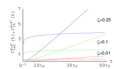
Figure 1: Figure shows $\Gamma^{p,p^{\prime}}_{vac}(t)$ and $\Gamma^{p,p^{\prime}}_{th}(t)$ as a function of $\zeta=2\alpha(\mbox{\boldmath$p$}-\mbox{\boldmath$p$}\,^{\prime})^{2}/3\pi m_{0}^{2}c^{2}$, in the case $T=300K$.

In the range where the vacuum contribution dominates ($t\ll\tau_{F}$) there are two different typical time dependencies. In the first one ($t\ll\Omega^{-1}$) the increase of decoherence is fast while in the second one ($t\gg\Omega^{-1}$) it slows into a logarithmic dependence. Fig. 2 represents the time development of $\exp[-\Gamma^{p,p^{\prime}}_{vac}(t)]$ as a function of the coupling constant $\alpha$, showing that by increasing $\alpha$ and fixed $\mbox{\boldmath$p$}-\mbox{\boldmath$p$}\,^{\prime}$, we observe a decay of matrix elements due to the vacuum contribution faster in time.

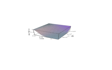
Figure 2: In figure it is plotted the time development of $\exp[-\Gamma^{p,p^{\prime}}_{vac}(t)]$ (20) as a function of the coupling constant $\alpha=e^{2}/\hslash c$ in the case $|\mbox{\boldmath$p$}-\mbox{\boldmath$p$}\,^{\prime}|/m_{0}c=0.1$. The time is taken in unit of $t\Omega$ and the range of $\alpha$ is chosen to visualize the vacuum effect on the decoherence.

We distinguish two different characteristic times of the decoherence process relative to the vacuum

$$\tau_{vac}=\frac{1}{\Omega}\;\exp\left[\frac{3\pi}{2\alpha}\frac{m_{0}^{2}c^{2}}{(\mbox{\boldmath$p$}-\mbox{\boldmath$p$}\,^{\prime})^{2}}\right]\,,$$ (28)

and to the thermal contribution

$$\tau_{th}=\tau_{F}\frac{3\pi}{2\alpha}\frac{m_{0}^{2}c^{2}}{(\mbox{\boldmath$p$}-\mbox{\boldmath$p$}\,^{\prime})^{2}}\,.$$ (29)

These characteristic times have the same form of those obtained for the decoherence of the interference pattern in Petruccione-Breuer libro 2002 .

The mass and charge parameters $m_{0}$ and $e$, appearing in $\tau_{vac}$ and $\tau_{th}$, are arbitrary. The only restriction is that they refer to a body that can be treated as a point like particle within the dipole approximation. For example, these parameters could represent the mass and the charge of a highly charged nucleus or even of a macroscopic body of linear dimensions small enough, and therefore $\alpha$ is a free parameter.

Let’s observe that the time at which vacuum and thermal decoherence are effective, depending of the value of the coupling constant $\alpha$, fall inside the time $\tau_{d}$ of validity of our model.

III.1.2 Analysis of $\Delta p(t)$ and $l_{p}(t)$

The above results are independent from the structure of the initial reduced density matrix elements $\rho^{p,p^{\prime}}_{S}(0)$. Now we specialize these results to the case of an initial Gaussian wave packet of spatial width $\Delta r$

$$\rho^{p,p^{\prime}}_{S}(0)=\mathrm{N}\>\exp\left\{-\frac{3\left[(\mbox{\boldmath$p$}-\mbox{\boldmath$p$}_{0})^{2}+(\mbox{\boldmath$p$}\,^{\prime}-\mbox{\boldmath$p$}_{0})^{2}\right]}{4\Delta p^{2}}\right.\\ \left.-i\frac{\mbox{\boldmath$r$}_{0}\cdot(\mbox{\boldmath$p$}-\mbox{\boldmath$p$}\,^{\prime})}{\hslash}\right\}\,,$$ (30)

with $\Delta p$ the width in the momentum space, $\mbox{\boldmath$p$}_{0}$ the initial average momentum of the particle, $\mathrm{N}=(\sqrt{3}/\sqrt{2\pi}\Delta p)^{3}$ the normalization factor and $\Delta r\Delta p=3\hslash/2$.
Substituting the gaussian wave packet of Eq. (30) in the reduced density matrix at time $t$ of Eq. (24), this can be put under the form

$$\hat{\rho}^{p,p^{\prime}}_{S}(t)=\mathrm{N}\exp\left(-\frac{3p_{0}^{2}}{2\Delta p^{2}}\right)$$ (31)

$$\times\exp\left[-\left(\Gamma(t)+\frac{3}{8\Delta p^{2}}\right)(\mbox{\boldmath$p$}-\mbox{\boldmath$p$}\,^{\prime})^{2}-\frac{3(\mbox{\boldmath$p$}+\mbox{\boldmath$p$}\,^{\prime})^{2}}{8\Delta p^{2}}\right.$$

$$\left.+i\Phi(t)(p^{2}-p^{\prime 2})+\frac{3\mbox{\boldmath$p$}_{0}\cdot(\mbox{\boldmath$p$}+\mbox{\boldmath$p$}\,^{\prime})}{2\Delta p^{2}}-i\frac{\mbox{\boldmath$r$}_{0}\cdot(\mbox{\boldmath$p$}-\mbox{\boldmath$p$}\,^{\prime})}{\hslash}\right].$$

A way to quantify the degree of loss of coherence of the wave packet is through the coherence length $l_{p}(t)$ Libro decoerenza 2002 , defined as the width of $\hat{\rho}_{S}(t)$ along the main skew diagonal, meaning the region inside which the coherence between momenta has not been yet destructed at time $t$. $l_{p}(t)$ may be compared with the width of $\hat{\rho}_{S}(t)$ along the diagonal that measures the wave packet width at a time $\Delta p(t)$, given by

$$\Delta p(t)=\sqrt{<p^{2}>_{t}-<p>_{t}^{2}}=\Delta p\,,$$ (32)

where we have used $<p^{2}>=\mathrm{tr}(\hat{\rho}_{S}(t)p^{2})=\Delta p^{2}+p_{0}^{2}$ and $<\hat{\mbox{\boldmath$p$}}>_{t}=\mathrm{tr}\{\hat{\rho}_{S}(t)\hat{\mbox{\boldmath$p$}}\}=\mbox{\boldmath$p$}_{0}$. Because $\Delta p(t)$ is constant the wave packet doesn’t spread with time in momentum space.

The coherence length $l_{p}(t)$, proportional to the inverse of the square root of the coefficient of $(\mbox{\boldmath$p$}-\mbox{\boldmath$p$}\,^{\prime})^{2}$ in Eq. (31) Libro decoerenza 2002 , is:

$$l_{p}(t)=\frac{\Delta p(t)}{\sqrt{1+8\Delta p^{2}\Gamma(t)/3}}\,.$$ (33)

To quantify the effective loss of coherence in the wave packet we study the ratio $l_{p}(t)/\Delta p(t)$. This quantity gives a measure of the relative width of the reduced density matrix off the diagonal compared with the width along the diagonal. Using Eq. (33) and the explicit form of $\Gamma(t)$ for $t>\tau_{F}$, given by Eq. (25), we obtain

$$\frac{l_{p}(t)}{\Delta p(t)}\approx\frac{3m_{0}c}{4\Delta p}\sqrt{\frac{\pi\tau_{F}}{\alpha\,t}},\quad\quad\quad\quad t\gg t^{*}$$ (34)

where $t^{*}=(3m_{0}c)^{2}\pi\tau_{F}/(4\Delta p)^{2}\alpha$. Being $\Delta p(t)$ constant in time, Eq. (34) shows that the coherence length for large times decreases going to 0 as $1/\sqrt{t}$ for $t\rightarrow\infty$. The decoherence process in momentum space is thus characterized by a complete decay of the off diagonal elements of the particle density matrix for large times while the populations remain constant.

This kind of behaviour of the reduced density matrix is shown in Fig. 3 obtained from Eq. (31).

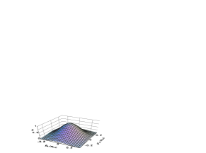
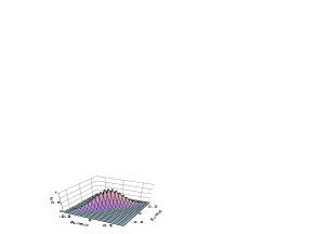
Figure 3: In figure it is represented the absolute value of the normalized density matrix $Z=|\rho^{{p_{x}},{p^{\prime}_{x}}}_{S}(t)|/N_{x}$ in one dimension, $N_{x}=1/\sqrt{2\pi}\Delta p_{x}$, with $p_{0}=0$ and $\Delta p_{x}/m_{0}c\approx 0.1$. On the top it is $t=0$ while on the bottom it is $t=3\tau_{vac}$, where $\tau_{vac}$ is taken for $p_{x}-p_{x}^{\prime}=\Delta p_{x}$.

III.2 Coordinate space

Our analysis is now extended to real space in order to describe spatial decoherence in more complex situations such as Young interference or Schrödinger cat states setups. We expect that changing representation the dynamics induced by the interaction with the electromagnetic field will appear more complex than in momentum space. As shown, in fact, it provides a basis of pointer states which allows a simple analysis of the process. To investigate the effects in the real space we need the reduced density matrix in the configuration space. It can be obtained from the corresponding momentum space reduced density matrix by performing a double Fourier transform:

$$\rho^{r,r^{\prime}}_{S}\!(t)\!=\!\frac{1}{(2\pi\hslash)^{3}}\!\!\int\!\!\mathrm{d}^{3}p\,\mathrm{d}^{3}p^{\prime}\rho^{p,p^{\prime}}_{S}\!(t)\exp\!\left[\frac{i}{\hslash}(\mbox{\boldmath$p$}\cdot\mbox{\boldmath$r$}-\mbox{\boldmath$p$}\,^{\prime}\cdot\mbox{\boldmath$r$}\,^{\prime})\right]\!.$$ (35)

Taking the Gaussian wave packet described by $\rho^{p,p^{\prime}}_{S}(0)$ of Eq. (30), the transform can be explicitly performed and is given in Appendix B. The spatial reduced density matrix $\rho^{r,r^{\prime}}_{S}(t)$, given by Eq. (B), can be rewritten as

$$\rho^{r,r^{\prime}}_{S}(t)=\frac{\mathrm{N}\Delta p^{3}}{\Delta r(t)^{3}}\>\exp\left[i\frac{\Delta r^{2}+6\Gamma(t)\hslash^{2}}{\Delta r(t)^{2}}\frac{\mbox{\boldmath$p$}_{0}\cdot(\mbox{\boldmath$q$}-\mbox{\boldmath$q$}\,^{\prime})}{\hslash}\right]$$

$$\times\exp\left\{-\frac{3[(\mbox{\boldmath$q$}-\langle\mbox{\boldmath$\hat{q}$}\rangle_{t})^{2}+(\mbox{\boldmath$q$}\,^{\prime}-\langle\mbox{\boldmath$\hat{q}$}\rangle_{t})^{2}]}{4\Delta r(t)^{2}}\right\}$$ (36)

$$\times\exp\left\{\frac{\Delta p^{2}}{\Delta r(t)^{2}}\left[-\Gamma(t)(\mbox{\boldmath$q$}-\mbox{\boldmath$q$}\,^{\prime})^{2}-i\Phi(t)(q^{2}-q^{\prime 2})\right]\right\}\,,$$

where: $\mbox{\boldmath$q$}=\mbox{\boldmath$r$}-\mbox{\boldmath$r$}_{0}$ is the displacement from the initial position and its average at the time $\langle\mbox{\boldmath$\hat{q}$}\rangle_{t}$ is given by

$$\langle\mbox{\boldmath$\hat{q}$}\rangle_{t}=\mathrm{tr}\{\hat{\rho}_{S}(t)\hat{q}\}=-2\mbox{\boldmath$p$}_{0}\Phi(t)\hslash\,,$$ (37)

$\Phi(t)$ and $\Gamma(t)$ are defined by Eqs. (III.1) and (III.1) while $\Delta r(t)$ is the spatial width of the wave packet at time $t$.
From Eq. (B) we get

$$\langle\hat{q}^{2}\rangle_{t} = \mathrm{tr}\{\hat{\rho}_{S}(t)\hat{q}^{2}\}$$

$$= \Delta r^{2}+6\Gamma(t)\hslash^{2}+\frac{9\Phi(t)^{2}\hslash^{4}}{\Delta r^{2}}+4p_{0}^{2}\Phi(t)^{2}\hslash^{2}\,,$$

and thus, using also Eq. (37), $\Delta r(t)$ is given by:

$$\Delta r(t) =\Delta q(t)=\sqrt{\langle\hat{q}^{2}\rangle_{t}-\langle\mbox{\boldmath$\hat{q}$}\rangle_{t}^{2}}$$

$$=\Delta r\sqrt{1+\frac{6\Gamma(t)\hslash^{2}}{\Delta r^{2}}+\frac{9\Phi(t)^{2}\hslash^{4}}{\Delta r^{4}}}\,.$$ (39)

$\Delta r(t)$ is at $t=0$, $\Delta r(0)=\Delta r$, and increases with time.

$\rho^{r,r^{\prime}}_{S}(t)$ can be obtained by its form at $t=0$

$$\rho^{r,r^{\prime}}_{S}\!(0)=\frac{\mathrm{N}\Delta p^{3}}{\Delta r^{3}}\>\exp\!\left[i\frac{\mbox{\boldmath$p$}_{0}\cdot(\mbox{\boldmath$q$}-\mbox{\boldmath$q$}\,^{\prime})}{\hslash}-\frac{3(q^{2}+q^{\prime 2})}{4\Delta r^{2}}\right],$$ (40)

replacing the initial width of the wave packet $\Delta r$ with its value at time $t$, $\Delta r(t)$, multiplying by $(\Delta r^{2}+6\Gamma(t)\hslash^{2})/\Delta r(t)^{2}$ the phase factor in the first exponent, centering the wave packet in the average displacement $\langle\mbox{\boldmath$\hat{q}$}\rangle_{t}$ in the second exponent and multiplying by an exponential factor which gives an increase of decoherence and a phase variation analogous to the factor appearing in the reduced momentum density matrix elements of Eq. (24).

III.2.1 Time dependent dressing

The average of the operator $\hat{\mbox{\boldmath$q$}}$ at time $t$, given by Eq. (37) and using the explicit form of $\Phi(t)$ (III.1), is

$$\langle\mbox{\boldmath$\hat{q}$}\rangle_{t}=\frac{\mbox{\boldmath$p$}_{0}t}{m_{0}}\left[1-\frac{4\alpha\hslash\left(\Omega-\frac{\arctan\Omega t}{t}\right)}{3\pi m_{0}c^{2}}\right]\,.$$ (41)

From this equation the average velocity of the wave packet is

$$\langle\hat{\dot{\mbox{\boldmath$q$}}}\rangle_{t}=\frac{\mathrm{d}}{\mathrm{d}t}\langle\mbox{\boldmath$\hat{q}$}\rangle_{t}=\frac{\mbox{\boldmath$p$}_{0}}{m_{0}}\left(1-\frac{4\alpha\hslash\Omega}{3\pi m_{0}c^{2}}\frac{\Omega^{2}t^{2}}{1+\Omega^{2}t^{2}}\right)\,.$$ (42)

As observed before, $\hat{\mbox{\boldmath$p$}}$ is a constant of motion, instead the velocity $\hat{\dot{\mbox{\boldmath$q$}}}=[\hat{\mbox{\boldmath$p$}}-e\mbox{\boldmath$\hat{A}$}(\mbox{\boldmath$r$}_{0})/c]/m_{0}$ it is not because it does not commute with the Hamiltonian (3). This may be related to the fact that, starting with uncoupled initial conditions, the charged particle is subject to time dependent dressing by the transverse photons. This increases its mass while $\hat{\mbox{\boldmath$p$}}$ remains constant. The mass variation can be obtained casting Eq. (42) in the form

$$\langle\hat{\dot{\mbox{\boldmath$q$}}}\rangle_{t}=\frac{\langle\mbox{\boldmath$\hat{p}$}\rangle_{t}}{m(t)}\approx\frac{\mbox{\boldmath$p$}_{0}}{m_{0}}\left[1-\frac{\delta m(t)}{m_{0}}\right]\,,$$ (43)

where $m(t)=m_{0}+\delta m(t)$ is the mass at time $t$ being the mass increase $\delta m(t)$ given by

$$\delta m(t)=\frac{4\alpha\hslash\Omega}{3\pi c^{2}}\frac{\Omega^{2}t^{2}}{1+\Omega^{2}t^{2}}\>\approx\>\left\{\>\begin{aligned} \frac{4\alpha\hslash\Omega}{3\,\pi\,c^{2}}\Omega^{2}t^{2},\quad\quad\,\textit{t}\ll\Omega^{-1}\\ \\ \frac{4\,\alpha\,\hslash\,\Omega}{3\,\pi\,c^{2}}\;.\;\;\;\;\;\quad\quad\textit{t}\gg\Omega^{-1}\end{aligned}\right.$$ (44)

For $t\ll\Omega^{-1}$ $\delta m(t)$ increases quadratically bellomo 2004 while for $t\gg\Omega^{-1}$ coincides with the usual total mass variation due to the interaction with the electromagnetic field Sakurai 1977 .

We observe that the equation of motion (41), from which we derived the expression for the mass increase, is related only to the total phase factor $\Phi(t)$ and is then temperature independent at first order in $v_{0}/c$.

III.2.2 Analysis of $\Delta r(t)$ and $l_{r}(t)$

The mass variation due to dressing is relevant if one wishes to compare the evolution of the wave packet width in the absence of interaction, $\Delta r(t)^{0}$, with its expression, $\Delta r(t)$, in the presence of interaction. In the last case we have from Eq. (III.2)

$$\Delta r(t) =\Delta r\sqrt{1+\frac{\Delta p^{2}t^{2}}{\Delta r^{2}}\frac{4\hslash^{2}\Phi(t)^{2}}{t^{2}}+\frac{6\Gamma(t)\hslash^{2}}{\Delta r^{2}}}\,,$$ (45)

with $\Gamma(t)$ and $\Phi(t)$ defined by Eqs. (III.1) and (III.1). Putting $e=0$ we obtain the well known expression for the free spread Pauli 2000

$$\Delta r(t)^{0}=\Delta r\sqrt{1+\frac{\Delta p^{2}t^{2}}{\Delta r^{2}}\frac{1}{m_{0}^{2}}}\,.$$ (46)

$\langle\mbox{\boldmath$\hat{q}$}\rangle_{t}$, given by Eq. (37), can also be obtained by integrating Eq. (43)

$$\langle\mbox{\boldmath$\hat{q}$}\rangle_{t}=-2\mbox{\boldmath$p$}_{0}\hslash\Phi(t)=\mbox{\boldmath$p$}_{0}\int_{0}^{t}\frac{1}{m(t^{\prime})}\mathrm{d}t^{\prime}\,.$$ (47)

Thus we can identify

$$\frac{-2\hslash\Phi(t)}{t}=\frac{1}{t}\int_{0}^{t}\frac{1}{m(t^{\prime})}\mathrm{d}t^{\prime}={\left\langle\frac{1}{m(t^{\prime})}\right\rangle}_{t}\,,$$ (48)

${\left\langle\frac{1}{m(t^{\prime})}\right\rangle}_{t}$ being the time average of $1/m(t^{\prime})$ over the time $t$. The width of the wave packet at time $t$ (45) can be thus rewritten as

$$\Delta r(t)=\Delta r\sqrt{1+\frac{\Delta p^{2}t^{2}}{\Delta r^{2}}{\left\langle\frac{1}{m(t^{\prime})}\right\rangle}_{t}^{2}+\frac{6\Gamma(t)\hslash^{2}}{\Delta r^{2}}}\,.$$ (49)

Eq. (49) shows that, starting from uncoupled condition, the interaction with the electromagnetic field induces differences with respect to the free evolution $\Delta r(t)^{0}$. The first one consists in the replacement of the inverse of the initial mass $1/m_{0}$ by ${\left\langle 1/m(t^{\prime})\right\rangle}_{t}$ and may be attributed to the $t$-dependent dressing. This effect is due to the vacuum fluctuations and is related to the total phase factor $\Phi(t)$, the mass increase leading to a rate decrease of the width with respect to the free case. The second effect is given by the term within the square root

$$\frac{6\Gamma(t)\hslash^{2}}{\Delta r^{2}}=\frac{1}{\Delta r^{2}}\frac{4\alpha\hslash^{2}}{\pi m_{0}^{2}c^{2}}\ln\left[\sqrt{1+\Omega^{2}t^{2}}\,\,\frac{\sinh(t/\tau_{F})}{t/\tau_{F}}\right]\,.$$ (50)

It always leads to an additional increase of the width of the wave packet. It contains both the effect of vacuum, represented by the term $\sqrt{1+\Omega^{2}t^{2}}$, and of the thermal field represented by the term $\sinh(t/\tau_{F})/(t/\tau_{F})$, being this last term for $T=0$ equal to $1$ ($\tau_{F}=\hslash/\pi k_{B}T$).

The comparison of the amplitudes of the vacuum and thermal terms in time may be obtained using the forms of the coefficients $\Gamma(t)$ and $\Phi(t)$ given by Eqs. (25) and (26) for small ($t\ll\Omega^{-1}$) and large ($t\gg\tau_{F}$) times . For small times the total effect is that the width of the wave packet results larger than in the free case. For large times, instead, the additional term becomes negligible and the spreading is slower than in the free case because the increasing of mass.

The space coherence length $l_{r}(t)$ represents the typical distance for which it is possible to have constructive interference among different parts within the wave packet. It can be read directly from the coefficient of $(\mbox{\boldmath$q$}-\mbox{\boldmath$q$}\,^{\prime})^{2}$ term of the reduced density matrix written under the form of Eq. (96), being in fact proportional to the inverse of this coefficient Libro decoerenza 2002 :

$$l_{r}(t)=\frac{\Delta r(t)}{\sqrt{1+6\hslash^{2}\Gamma(t)/\Delta r^{2}}}.$$ (51)

Using Eq. (III.2) for $\Delta r(t)$ it results that $l_{r}(t)$ increases with time, while, analogously to what happens in momentum space (33), $l_{r}(t)/\Delta r(t)$ decreases with time because $\Gamma(t)$ increases with time (III.1). In absence of interaction $\Gamma(t)$ is equal to zero and therefore the free space coherence length, $l_{r}(t)^{0}$, is always equal to the width of the wave packet which increases coherently in time due to the well known free spread (46). The coupling with the field induces an evolution of $l_{r}(t)$ different from $\Delta r(t)$. Using Eqs. (33) and (51) and $\Delta r\Delta p=3\hslash/2$, it follows that $l_{r}(t)/\Delta r(t)=l_{p}(t)/\Delta p(t)$ and therefore Eq. (34) describes also in the coordinate space the behaviour of the coherence length with respect to the width of the wave packet for large times. This equation shows that the ratio decreases to zero as $1/\sqrt{t}$ for $t\rightarrow\infty$ describing a loss of coherence also in the configuration space.

Another interesting aspect to investigate is the behaviour of $l_{r}(t)$ with respect to its evolution in the free case $l_{r}(t)^{0}$. Using Eq. (46) for $l_{r}(t)^{0}$ and Eqs. (51) and (49) we can put the coherence length in the form:

$$l_{r}^{2}(t) =\Delta r^{2}+\Delta p^{2}t^{2}{\left\langle\frac{1}{m(t^{\prime})}\right\rangle}_{t}^{2}\frac{\Delta r^{2}}{\Delta r^{2}+6\Gamma(t)\hslash^{2}}<l_{r}^{2}(t)^{0}\,.$$ (52)

Eq. (52) shows that dressing induces a slower increase of coherence length due to the mass increase, but always maintaining the coherence, while vacuum and thermal field induce a destruction of coherence in space such that the coherence length is lower than in the free evolution case.

In the momentum space we obtained a simple dynamics: the width of the wave packet remains constant while the coherence length decreases with respect to its initial value going to zero. In coordinate space, instead, different factors contribute to the dynamics: free evolution contributes to the coherent increase of the width of the wave packet coherently and therefore of the coherence length; the particle time dependent dressing of the particle slows this increase; finally vacuum and thermal field induce a loss of space coherence such that the value of the space coherence length in presence of the interaction is always lower than its value in absence of the interaction.

III.2.3 Linear entropy

The dynamics of our system is described by the reduced density matrix time evolution as a transformation from the pure initial state (10) into a statistical mixture (24). The time dependence of this process, that implies a loss of information on the system, may be described by the so-called linear entropy, $S_{\mathrm{lin}}$ Petruccione-Breuer libro 2002 . It has been analyzed in the case of localization by scattering, to measure how strongly the environment destroys coherence between positions by delocalizing phases, finding a linear departure in time from the initial value $0$ describing a pure state Libro decoerenza 2002 . Using its definition we obtain here

$$S_{\mathrm{lin}}=\mathrm{tr}(\hat{\rho}_{S}-\hat{\rho}_{S}^{2})=1-\sqrt{\frac{1}{1+6\Gamma(t)\hslash^{2}/\Delta r^{2}}}\,,$$ (53)

which describes the loss of purity of the initial state. It is interesting to note that in the case of initial Gaussian wave packet Morikawa 1990 , $S_{\mathrm{lin}}$ is directly connected to a dimensionless measurement of the decoherence given by the ratio between the decoherence length and the wave packet width. This ratio coincides both in the $p$ and $r$ representations (33) and (51) and using Eq. (53) may be expressed as

$$S_{\mathrm{lin}}=1-\frac{l_{p}(t)}{\Delta p(t)}=1-\frac{l_{r}(t)}{\Delta r(t)}\,.$$ (54)

Using Eq. (33) and the approximated form of $\Gamma(t)$ for small times given by Eq. (25), we find that $S_{lin}$ at the beginning evolves quadratically from the initial value $0$ corresponding to a pure state, then slows and finally (34) goes to 1 for $t\rightarrow\infty$ as $1-1/\sqrt{t}$.

In Fig. 4 the time development of the linear entropy is plotted as a function of the coupling constat $\alpha$. The figure shows clearly that the increase of this quantity towards 1 depends strongly on $\alpha$, that is on the charge of the particle considered.

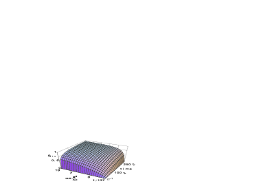
Figure 4: In figure it is shown the behaviour of $S_{\mathrm{lin}\mathrm{}}$ in time as a function of $\alpha$.

IV Interpretation of vacuum induced decoherence

The temperature independent part of decoherence is represented by $\Gamma^{p,p^{\prime}}_{vac}(t)$ of Eq. (20). In the following we shall analyze the processes that contribute to $\Gamma^{p,p^{\prime}}_{vac}(t)$.

In the case of a charged particle, initially described by a wave function made of a coherent superposition of two moving wave packets, it has been previously shown Breuer-Petruccione 2001 that Bremsstrahlung radiation induces decoherence decreasing the visibility of the interference pattern that results from their overlapping. The reason is that in its trajectory the particle is subject to a sudden change of the 4-momentum and in this process it is radiated as Bremsstrahlung photons the energy Peskin-Schroder 1995 :

$$E_{R}=\frac{\alpha}{\pi}k_{max}I(v,v^{\prime})\,,$$ (55)

where $I(v,v^{\prime})$ is a function of the initial and final velocity and $k_{max}$ is the wave vector corresponding to the frequency equals to the reciprocal of the time scattering during which the 4-momentum changes. This energy results, as also the decoherence function, proportional to $\alpha$. Thus Bremsstrahlung may be hold responsible of decoherence.

In our system the particle is also subject to a change of velocity during the dressing process with the emission of Bremsstrahlung photons. These could be held responsible of the temperature independent loss of coherence between the momentum components of the wave packet. However the radiation energy emitted in the unity of time from the accelerated charged particle during the dressing process can be estimated as Rossi 1991 :

$$E_{B}\propto\frac{e^{2}\langle\hat{\ddot{\mbox{\boldmath$q$}}}\rangle^{2}}{c^{3}}=\alpha\frac{\hslash\langle\hat{\ddot{\mbox{\boldmath$q$}}}\rangle^{2}}{c^{2}}\,,$$ (56)

with $\langle\hat{\ddot{\mbox{\boldmath$q$}}}\rangle$ being the average acceleration of the particle. To obtain $\langle\hat{\ddot{\mbox{\boldmath$q$}}}\rangle$ during the dressing we take the time derivative of Eq. (42):

$$\langle\hat{\ddot{\mbox{\boldmath$q$}}}\rangle=-\frac{\mbox{\boldmath$p$}_{0}}{m_{0}^{2}}\frac{4\,\alpha\,\hslash\,\Omega}{3\,\pi\,c^{2}}\frac{2\Omega^{2}t}{\left(1+\Omega^{2}t^{2}\right)^{2}}\,.$$ (57)

Substituting this last equation in Eq. (56) the estimated emitted energy per unity of time results proportional to $\alpha^{3}$. The vacuum contribution to the decoherence function is shown from Eq. (20) to be proportional to $\alpha$. From the considerations above it follows that the emission of Bremsstrahlung photons doesn’t seem to be relevant for the vacuum decoherence process.

However let’s observe that for short times ($t\ll\Omega^{-1}$), the decoherence factor $\Gamma(t)$ of Eq. (25) and the mass variation $\delta m(t)$ of Eq. (44) show both the same $t$ and $\alpha$ dependence. This appears to suggest a connection between the decoherence process for small times (vacuum contribution) and the dressing process. In analogy to the case of the two level systems Palma-Suominen-Ekert 1996 , the link between dressing and vacuum induced decoherence could be attributed to the correlation that get established between each component $p$ of the wave packet and the part of the dressing structure of the transverse electromagnetic field associated to it.

To verify this hypothesis, we shall analyze the evolution of the field associated to each component of the wave packet, during the initial phase of the decoherence process.

IV.1 Field structure dynamics

In the analyses of decoherence the behaviour of the environment is usually not investigated being the interest placed on the system evolution. In our case the environment is the electromagnetic field and its behaviour during the decoherence process can be analyzed by performing the trace of the total density matrix over the degrees of freedom of the particle.

For calculation purposes we shall consider the initial wave packet of momentum width $\Delta p$ as a sum of momentum sharp wave packets of width $\Delta\bar{p}\ll\Delta p$. Each of these sharp wave packets is centered at a momentum $\bar{\mbox{\boldmath$p$}}$ and it has in configuration space a width $\Delta\bar{r}\approx\hslash/\Delta\bar{p}$ taken less than $c/\Omega$ so that the dipole approximation can be yet used. To describe the development of the field correlated to one of these sharp wave packets centered at $\bar{\mbox{\boldmath$p$}}$ we start from a totally decoupled initial condition. The field is taken in its vacuum state and the charged particle is described by a sharp wave packet with momentum components peaked around $\bar{\mbox{\boldmath$p$}}$ of the form $\sqrt{N_{\varepsilon}}\sum_{p}\delta^{\varepsilon}_{p,\bar{p}}|p\rangle$, where $N_{\varepsilon}$ is a normalization factor and $\delta^{\varepsilon}_{p,\bar{p}}$ indicates a quasi delta centered on $\bar{\mbox{\boldmath$p$}}$ of width $\Delta\bar{p}$.

The corresponding initial density matrix is

$$\hat{\rho}(0) =\hat{\rho}_{S}(0)\otimes|\{0_{\bar{k},\bar{j}}\}\rangle\langle\{0_{\dot{k},\dot{j}}\}|$$

$$=\sum_{p,p^{\prime}}|p\rangle\bar{N}\delta^{\varepsilon}_{p,\bar{p}}\delta^{\varepsilon^{\prime}}_{p^{\prime},\bar{p}}\langle p^{\prime}|\otimes|\{0_{\bar{k},\bar{j}}\}\rangle\langle\{0_{\dot{k},\dot{j}}\}|\,.$$ (58)

We shall consider the representation of $\hat{\rho}(t)$ in a coherent basis. Indicating with $|\lambda_{k,j}\rangle$ a coherent state of the mode $\{\mbox{\boldmath$k$},j\}$ of amplitude $\lambda$, the reduced density matrix elements of the field in this basis, with the initial condition of Eq. (IV.1), are given by

$$\hat{\rho}_{F}^{\lambda_{k,j},\lambda^{\prime}_{k^{\prime},j^{\prime}}}(t)=\langle\lambda_{k,j}|\mathrm{tr}_{S}\{\hat{U}(t)\hat{\rho}_{S}(0)\otimes|\{0_{\bar{k},\bar{j}}\}\rangle\\ \langle\{0_{\dot{k},\dot{j}}\}|\hat{U}^{-1}(t)\}|\lambda^{\prime}_{k^{\prime},j^{\prime}}\rangle\,.$$ (59)

The explicit calculation, reported in Appendix C by Eq. (103), gives for the reduced density matrix of the field

$$\hat{\rho}_{F}^{\lambda_{k,j},\lambda^{\prime}_{k^{\prime},j^{\prime}}}(t)=N_{\varepsilon}\exp\left[-\frac{|\lambda_{k,j}|^{2}}{2}-\frac{|\lambda^{\prime}_{k^{\prime},j^{\prime}}|^{2}}{2}-\frac{|\beta_{k,j}^{\bar{p}}|^{2}}{2}\right.\\ \left.-\frac{|\beta_{k^{\prime},j^{\prime}}^{\bar{p}}|^{2}}{2}+\lambda^{*}_{k,j}\beta_{k,j}^{\bar{p}}+\lambda^{\prime}_{k^{\prime},j^{\prime}}\beta_{k^{\prime},j^{\prime}}^{{\bar{p}}*}\right]\,,$$ (60)

with $\beta_{k,j}^{\bar{p}}$ defined in Eq. (98). Because of our choice of sharp wave packets in $p$ space, the density matrix of Eq. (60) retains only a dependence on $\bar{p}$.

Eq. (60) allows to get the average number of photons $\langle\hat{n}_{\bar{p}}\rangle$ that can be associated to each sharp wave packet of width $\Delta\bar{p}$ and centered at the momentum $\bar{\mbox{\boldmath$p$}}$ of the total wave packet. The calculation, performed in Appendix C by (113), leads to

$$\langle\hat{n}_{\bar{p}}\rangle=\frac{2\alpha}{3\pi}\frac{{\bar{p}}^{2}}{m_{0}^{2}c^{2}}\ln\left(1+\Omega^{2}t^{2}\right)\,.$$ (61)

The time dependence of the average number of photons of Eq. (61) is, apart a factor 2, equal to that of the vacuum contribution to the decoherence function (20). This result appears to give a strong indication that it is just the buildup of correlations among the various momenta that compose the wave packet and the corresponding associated transverse photons that leads to vacuum decoherence in our system.

To confirm the possibility of associating a number of photons to the various momentum components of a given wave packet, we could choose as initial state a sum of two sharp wave packets of width $\Delta\bar{p}$ peaked around two different momenta. In this case it is easy to show that the average number of photons surrounding the particle can be written as a sum of two terms relative to the two sharp wave packets composing the initial state.

The energy associated to the field structure that builds up around the particle is responsible together with the interaction energy of the mass variation $\delta m$ computed in Eq. (44). The average energy associated to the cloud of photons, obtained in Appendix C by (C), is equal to

$$\langle\hat{E}_{F}\rangle=\frac{8\alpha}{3\pi}\frac{\hslash\Omega}{m_{0}c^{2}}\frac{\Omega^{2}t^{2}}{1+\Omega^{2}t^{2}}\frac{{\bar{p}}^{2}}{2m_{0}}\,.$$ (62)

$\langle\hat{E}_{F}\rangle$ can be written, using Eq. (44) for $\delta m$, as $\langle\hat{E}_{F}\rangle=-({\bar{p}}^{2}/2m_{0})\times(\delta_{F}m/m_{0})$ with $\delta_{F}m=-2\delta m$. Therefore $\langle\hat{E}_{F}\rangle$ reflects on one side the build up of correlations with momenta and on the other side contributes to the mass variation. This explains the analogous time behaviour of $\delta m(t)$ and $\Gamma_{vac}(t)$.

V Summary and Conclusions

We have considered a free charged particle interacting with a bath consisting of an electromagnetic field at temperature $T$. We have analyzed the decoherence on the charged particle wave packet induced by the interaction through the investigation of the off diagonal elements of the particle reduced density matrix. The interaction has been taken in the minimal coupling form and the particle is described by a wave packet of width $\Delta r$. The effect of all the modes of wavelength larger than $\Delta r$ can be taken into account within the dipole approximation. The dipole approximation and the neglecting of the quadratic potential term reduces the coupling to a linear form and this in turn allows an exact treatment of the dynamics of the system.

Our analysis has been conducted in the context of non relativistic QED which is in the spirit of modern quantum field theory an effective low energy theory with the cut off frequency $\Omega$ parameterizing the physics due to the higher frequencies Zee 2003 . For this reason our final results must show a dependence on $\Omega$, that is however as usual weak (logarithmic), as for example in the case of non relativistic expression for the Lamb shift.

The analysis of the decoherence process has been conducted both in the momentum and configuration space and it has been possible to separate both the vacuum and the thermal contribution to decoherence.

In momentum space decoherence among different momentum components occurs without population decay, therefore decoherence occurs in its purest form that is without dissipation. This is reflected by the fact that the width $\Delta p(t)$ of the wave packet remains constant in time while the coherence length $l_{p}(t)$ decreases in time, in particular as $1/\sqrt{t}$ for large $t$.

In configuration space again both vacuum and thermal contribution appear in the decay of the off diagonal elements of the reduced density matrix similarly to what occurs in the momentum space. However in the characterization of the development of decoherence by the behaviour of the space width of the wave packet, $\Delta r(t)$, and the coherence length, $l_{r}(t)$, it is necessary to consider that in these quantities two contributions appear, which are not present in the momentum space. The first is due to the free evolution of the wave packet and the second to the dressing process. The appearance of these contributions only in the configuration space is due to the fact that the Hamiltonian commutes with each momentum component that then results to be a constant of the motion. In particular the dressing process, with the emission and absorption of virtual photons and the creation of a structure of transverse field around the particle, doesn’t modify the distribution of momenta of the wave packet while it modifies the spatial probability distribution. We have determined the contribution of these physical effects to $\Delta r(t)$ and $l_{r}(t)$.

We have tried to determine the physical effect responsible for the part of decoherence independent from the temperature. The Bremsstrahlung photons emitted during the dressing have been shown not to be relevant for vacuum decoherence. The results obtained about the particle mass variation indicate that the vacuum contribution to decoherence is temporally linked to the dressing process. We have shown by the analysis of the field structure dynamics that the onset of time dependent correlations, induced by the interaction, between the momentum components of the particle wave packet and the associated field structure, may be held responsible of vacuum induced decoherence. In fact the average number of entangled photons with a given momentum has the same time dependence of the vacuum part of the decoherence function and moreover has the same dependence on the physical parameters of the system.

The results obtained for our system on the development of induced decoherence depend on the fact that in the initial state considered there are not particle-field correlations. Previously it has been shown that decoherence evolution is influenced by the presence of initial partial correlation bellomo2 2005 ; Smith-Caldeira 1990 ; Romero-Paz 1997 ; Lutz 2003 . It appears of interest to analyze in which way the results obtained in this paper are modified in the more realistic case in which partial correlations between the system and the environment are present since the beginning.

Appendix A

A.1 Phase factor

In order to compute the phase factor $\xi(p,t)$ of Eq. (II.1) it is necessary to explicit the commutator of $\hat{H}_{I}$ at different times (7). Using the following relation satisfied by the polarization vectors

$$\sum_{j}\varepsilon_{k,j}^{m}\varepsilon_{k,j}^{n}=\delta_{m,n}-\check{\mbox{\boldmath$k$}}_{m}\check{\mbox{\boldmath$k$}}_{n}\,,$$ (63)

where $\check{\mbox{\boldmath$k$}}$ indicates the versor of $k$ and $m$ and $n$ are generical components, we obtain

$$\sum_{j}|\mbox{\boldmath$p$}\cdot\mbox{\boldmath$\varepsilon$}_{k,j}|^{2}=p^{2}-(\mbox{\boldmath$p$}\cdot\check{\mbox{\boldmath$k$}})^{2}\,.$$ (64)

By using the explicit form of the coupling coefficients of Eq. (4), and Eq. (64) to compute the sum over the polarizations, the commutator of $\hat{H}_{I}$ at different times (7) assumes the form

$$[\hat{H}_{I}(s),\hat{H}_{I}(s^{\prime})]\!=\!-2i\!\sum_{p,k,j}\!g_{k,j}^{p\,2}\hat{\sigma}_{p}\sin\left[(\omega_{k}-\mbox{\boldmath$k$}\cdot\mbox{\boldmath$v$}_{0})(s-s^{\prime})\right]$$

$$=\!-i\frac{4\pi e^{2}\hslash}{m_{0}^{2}V}\!\sum_{p,k}\!\frac{p^{2}-(\mbox{\boldmath$p$}\cdot\check{\mbox{\boldmath$k$}})^{2}}{\omega_{k}}\hat{\sigma}_{p}\sin\left[(\omega_{k}-\mbox{\boldmath$k$}\cdot\mbox{\boldmath$v$}_{0})(s-s^{\prime})\right].$$ (65)

The time integrations present in Eq. (II.1) give

$$\int_{0}^{t}\mathrm{d}s\int_{0}^{t}\mathrm{d}s^{\prime}\sin\left[(\omega_{k}-\mbox{\boldmath$k$}\cdot\mbox{\boldmath$v$}_{0})(s-s^{\prime})\right]\theta(s-s^{\prime})\\ =\frac{1}{(\omega_{k}-\mbox{\boldmath$k$}\cdot\mbox{\boldmath$v$}_{0})}\left[t-\frac{\sin(\omega_{k}-\mbox{\boldmath$k$}\cdot\mbox{\boldmath$v$}_{0})t}{(\omega_{k}-\mbox{\boldmath$k$}\cdot\mbox{\boldmath$v$}_{0})}\right]\,,$$ (66)

and joining Eqs. (66), (A.1) and (II.1) we obtain for $\xi(p,t)$

$$\xi(p,t)=\frac{2\pi\,e^{2}}{m_{0}^{2}V\hslash}\sum_{k}\frac{p^{2}-(\mbox{\boldmath$p$}\cdot\check{\mbox{\boldmath$k$}})^{2}}{\omega_{k}(\omega_{k}-\mbox{\boldmath$k$}\cdot\mbox{\boldmath$v$}_{0})}\\ \times\left[t-\frac{\sin(\omega_{k}-\mbox{\boldmath$k$}\cdot\mbox{\boldmath$v$}_{0})t}{(\omega_{k}-\mbox{\boldmath$k$}\cdot\mbox{\boldmath$v$}_{0})}\right]\,.$$ (67)

By taking the continuum limit on the field modes, $\sum_{k}\rightarrow V\int_{0}^{\infty}\mathrm{d}^{3}k/(2\pi)^{3}$, Eq. (67) becomes

$$\xi(p,t)=\frac{e^{2}}{\hslash m_{0}^{2}(2\pi)^{2}}\int\mathrm{d}^{3}k\left[t-\frac{\sin(\omega-\mbox{\boldmath$k$}\cdot\mbox{\boldmath$v$}_{0})t}{(\omega-\mbox{\boldmath$k$}\cdot\mbox{\boldmath$v$}_{0})}\right]\\ \times\frac{p_{x}^{2}(1-\check{\mbox{\boldmath$k$}}^{2}_{x})+p_{y}^{2}(1-\check{\mbox{\boldmath$k$}}^{2}_{y})+p_{z}^{2}(1-\check{\mbox{\boldmath$k$}}^{2}_{z})}{\omega(\omega-\mbox{\boldmath$k$}\cdot\mbox{\boldmath$v$}_{0})}\,.$$ (68)

By introducing the cut off factor $\exp(-\omega/\Omega)$, Eq. (68) assumes the form

$$\xi(p,t)= \frac{e^{2}}{4\pi^{2}\hslash m_{0}^{2}c^{3}}\int_{0}^{\infty}\frac{\mathrm{d}\omega}{\omega}\exp\left(-\frac{\omega}{\Omega}\right)$$ (69)

$$\times\int\mathrm{d}o\frac{\omega t(1-X)-\sin\left[\omega t(1-X)\right]}{{(1-X)^{2}}}$$

$$\times\left[p_{x}^{2}(1-\check{\mbox{\boldmath$k$}}^{2}_{x})+p_{y}^{2}(1-\check{\mbox{\boldmath$k$}}^{2}_{y})+p_{z}^{2}(1-\check{\mbox{\boldmath$k$}}^{2}_{z})\right]\,,$$

where $\mathrm{d}o=\sin\theta\mathrm{d}\theta\mathrm{d}\varphi$ is the infinitesimal solid angle and we have posed

$$\mbox{\boldmath$k$}\cdot\mbox{\boldmath$v$}_{0}=\omega\frac{v_{0}}{c}\left[\sin\theta_{0}\sin\theta_{k}\cos(\varphi_{k}-\varphi_{0})+\cos\theta_{0}\cos\theta_{k}\right]\\ =\omega X\,,$$ (70)

where $\theta_{0}$ and $\varphi_{0}$ are the angles of the vector $\mbox{\boldmath$v$}_{0}$ and $\theta_{k}$ and $\varphi_{k}$ are the angles of the vector $k$.
Indicating with $f(X)$ the $X$ dependent part within the integrand in Eq. (69), for small values of $v_{0}/c$, this can be expanded with respect to $X$ obtaining up to the first order in $X$

$$f(X)=\frac{\omega t(1-X)-\sin\left[\omega t(1-X)\right]}{{(1-X)^{2}}}\\ \approx\omega t-\sin\omega t+f^{\prime}(0)X\,.$$ (71)

Using this expansion and the following integrals

$$\int\mathrm{d}o(1-\check{\mbox{\boldmath$k$}}^{2}_{i})=\frac{8}{3}\pi\,,\qquad\mathrm{for}\;i=x,y,z\,,$$ (72)

$$\int\mathrm{d}o(1-\check{\mbox{\boldmath$k$}}^{2}_{i})X=0\qquad\mathrm{for}\;i=x,y,z\,,$$ (73)

in Eq. (69), we obtain up to first order in $v_{0}/c$

$$\xi(p,t) =\frac{2e^{2}p^{2}}{3\pi\hslash m_{0}^{2}c^{3}}\int_{0}^{\infty}\frac{\mathrm{d}\omega}{\omega}\exp\left(-\frac{\omega}{\Omega}\right)\left(\omega t-\sin\omega t\right)$$

$$=\frac{2\alpha p^{2}}{3\pi m_{0}^{2}c^{2}}(\Omega t-\arctan\Omega t)\,,$$ (74)

where $\alpha=e^{2}/\hslash c$ is a dimensionless coupling constant.

A.2 Decoherence function

To obtain the explicit expression of $\Gamma^{p,p^{\prime}}(t)$ (15) it is necessary to calculate the trace on the field

$$\chi(\gamma_{k,j}^{p,p^{\prime}},\gamma_{k,j}^{p,p^{\prime}}*)=\mathrm{tr}_{F}\left\{\exp\left(\hat{\mathrm{a}}^{{\dagger}}_{k,j}\gamma_{k,j}^{p,p^{\prime}}-\hat{\mathrm{a}}_{k,j}\gamma_{k,j}^{p,p^{\prime}}*\right)\hat{\rho}_{F}\right\}\,.$$ (75)

The operator $\exp\left(\hat{\mathrm{a}}^{{\dagger}}_{k,j}\gamma_{k,j}^{p,p^{\prime}}-\hat{\mathrm{a}}_{k,j}\gamma_{k,j}^{p,p^{\prime}}*\right)$ is the generator of the coherent states of amplitude $\gamma_{k,j}^{p,p^{\prime}}$. It has been shown Privman-Mozyrsky 1998 ; Petruccione-Breuer libro 2002 that Eq. 75 can be put in the form

$$\chi(\gamma_{k,j}^{p,p^{\prime}},\gamma_{k,j}^{p,p^{\prime}}*)=\exp\left\{-\frac{1}{2}|\gamma_{k,j}^{p,p^{\prime}}|^{2}\mathrm{tr}_{F}\!\left[\{\hat{\mathrm{a}}_{k,j},\hat{\mathrm{a}}^{{\dagger}}_{k,j}\}\hat{\rho}_{F}\right]\right\}.$$ (76)

Using Eqs. (75) and (76), the relation Petruccione-Breuer libro 2002

$$\mathrm{tr}_{F}\left[\{\hat{\mathrm{a}}_{k,j},\hat{\mathrm{a}}^{{\dagger}}_{k,j}\}\hat{\rho}_{F}\right]=\coth\left(\frac{\hslash\omega_{k}}{2k_{B}T}\right)$$ (77)

obtained in the case of thermal distribution for $\hat{\rho}_{F}$ and

$$|\gamma_{k,j}^{p,p^{\prime}}|^{2}=\left[(\mbox{\boldmath$p$}-\mbox{\boldmath$p$}\,^{\prime})\cdot\varepsilon_{k,j}\right]^{2}\frac{\left[1-\cos(\omega_{k}-\mbox{\boldmath$k$}\cdot\mbox{\boldmath$v$}_{0})t\right]}{\hslash\omega_{k}(\omega_{k}-\mbox{\boldmath$k$}\cdot\mbox{\boldmath$v$}_{0})^{2}}\frac{4\pi\,e^{2}}{m_{0}^{2}V}\,,$$ (78)

derived from the position following Eq. (15) and using Eqs. (4) and (9), the decoherence function (15) can be put in the form

$$\Gamma^{p,p^{\prime}}(t)=\frac{2\pi\,e^{2}}{\hslash m_{0}^{2}V}\sum_{k}\frac{\left[1-\cos(\omega_{k}-\mbox{\boldmath$k$}\cdot\mbox{\boldmath$v$}_{0})t\right]}{\omega_{k}(\omega_{k}-\mbox{\boldmath$k$}\cdot\mbox{\boldmath$v$}_{0})^{2}}\\ \times\coth\left(\frac{\hslash\omega_{k}}{2k_{B}T}\right)\sum_{j}\left[(\mbox{\boldmath$p$}-\mbox{\boldmath$p$}\,^{\prime})\cdot\varepsilon_{k,j}\right]^{2}\,.$$ (79)

Taking the continuum limit on the field modes $\sum_{k}\rightarrow V\int_{0}^{\infty}\mathrm{d}^{3}k/(2\pi)^{3}$, using $\sum_{j}\left[(\mbox{\boldmath$p$}-\mbox{\boldmath$p$}\,^{\prime})\cdot\varepsilon_{k,j}\right]^{2}=(\mbox{\boldmath$p$}-\mbox{\boldmath$p$}\,^{\prime})^{2}-\left[(\mbox{\boldmath$p$}-\mbox{\boldmath$p$}\,^{\prime})\cdot\check{\mbox{\boldmath$k$}}\right]^{2}$, inserting the cut off factor $\exp(-\omega/\Omega)$ and introducing the variable $X$ defined in Eq. (70), we obtain

$$\Gamma^{p,p^{\prime}} (t)=\frac{e^{2}}{4\pi^{2}\hslash m_{0}^{2}c^{3}}\int_{0}^{\infty}\frac{\mathrm{d}\omega}{\omega}\exp\left(-\frac{\omega}{\Omega}\right)\coth\left(\frac{\hslash\omega}{2k_{B}T}\right)$$

$$\times\int\mathrm{d}o\frac{1-\cos\left[\omega t(1-X)\right]}{(1-X)^{2}}\left[(\mbox{\boldmath$p$}-\mbox{\boldmath$p$}\,^{\prime})_{x}^{2}(1-\check{\mbox{\boldmath$k$}}^{2}_{x})\right.$$

$$\left.+(\mbox{\boldmath$p$}-\mbox{\boldmath$p$}\,^{\prime})_{y}^{2}(1-\check{\mbox{\boldmath$k$}}^{2}_{y})+(\mbox{\boldmath$p$}-\mbox{\boldmath$p$}\,^{\prime})_{z}^{2}(1-\check{\mbox{\boldmath$k$}}^{2}_{z})\right]\,,$$ (80)

where, as before, $\mathrm{d}o$ is the infinitesimal solid angle.
Indicating with $g(X)$ the $X$ dependent part within the integrand in Eq. (A.2), for small values of $v_{0}/c$, this can be expanded with respect to $X$ obtaining up to the first order in $X$

$$g(X)=\frac{1-\cos\left[\omega t(1-X)\right]}{(1-X)^{2}}\approx 1-\cos\omega t+g^{\prime}(0)X\,.$$ (81)

Using this expansion and Eqs. (72) and (73) to compute the angular integral in Eq. (A.2), we obtain up to first order in $v_{0}/c$

$$\Gamma^{p,p^{\prime}}(t)=\frac{2\alpha}{3\pi}\frac{(\mbox{\boldmath$p$}-\mbox{\boldmath$p$}\,^{\prime})^{2}}{m_{0}^{2}c^{2}}\int_{0}^{\infty}\frac{\mathrm{d}\omega}{\omega}\exp\left(-\frac{\omega}{\Omega}\right)\\ \times(1-\cos\omega t)\coth\left(\hslash\omega/2k_{B}T\right)\,.$$ (82)

Before carrying out the frequency integral in Eq. (82), we separate $\Gamma^{p,p^{\prime}}(t)$ in two parts, $\Gamma^{p,p^{\prime}}(t)=\Gamma^{p,p^{\prime}}_{vac}(t)+\Gamma^{p,p^{\prime}}_{th}(t)$: a temperature independent part due to vacuum fluctuations and a dependent one due to the thermal bath properties, which goes to zero for $T\rightarrow 0$. From Eq. (82) we obtain the temperature independent contribution as

$$\Gamma^{p,p^{\prime}}_{vac}(t) =\frac{2\alpha}{3\pi}\frac{(\mbox{\boldmath$p$}-\mbox{\boldmath$p$}\,^{\prime})^{2}}{m_{0}^{2}c^{2}}\int_{0}^{\infty}\mathrm{d}\omega\exp\left(-\frac{\omega}{\Omega}\right)\frac{(1-\cos\omega t)}{\omega}$$

$$=\frac{2\alpha}{3\pi}\frac{(\mbox{\boldmath$p$}-\mbox{\boldmath$p$}\,^{\prime})^{2}}{m_{0}^{2}c^{2}}\ln\sqrt{1+\Omega^{2}t^{2}}\,,$$ (83)

and the thermal contribution as

$$\Gamma^{p,p^{\prime}}_{th}(t)= \frac{2\alpha}{3\pi}\frac{(\mbox{\boldmath$p$}-\mbox{\boldmath$p$}\,^{\prime})^{2}}{m_{0}^{2}c^{2}}\int_{0}^{\infty}\frac{\mathrm{d}\omega}{\omega}\exp\left(-\frac{\omega}{\Omega}\right)(1-\cos\omega t)$$

$$\times[\coth\left(\hslash\omega/2k_{B}T\right)-1]$$

$$= \frac{2\alpha}{3\pi}\frac{(\mbox{\boldmath$p$}-\mbox{\boldmath$p$}\,^{\prime})^{2}}{m_{0}^{2}c^{2}}\frac{1}{\beta}\int_{0}^{t}\mathrm{d}s\int_{0}^{\infty}\mathrm{d}x\exp\left(-\frac{k_{B}Tx}{\hslash\Omega}\right)$$

$$\times[\coth\left(x/2\right)-1]\sin(sx/\beta)\,.$$ (84)

For $k_{B}T\ll\hslash\Omega$ and introducing $\tau_{F}=\hslash/\pi k_{B}T\approx 2.43\cdot 10^{-12}s/T[K]$, we find

$$\Gamma^{p,p^{\prime}}_{th}(t)\approx \frac{2\alpha}{3\pi}\frac{(\mbox{\boldmath$p$}-\mbox{\boldmath$p$}\,^{\prime})^{2}}{m_{0}^{2}c^{2}}\frac{1}{\beta}\int_{0}^{t}\mathrm{d}s\int_{0}^{\infty}\mathrm{d}x$$

$$\times[\coth\left(x/2\right)-1]\sin(sx/\beta)$$

$$= \frac{2\alpha}{3\pi}\frac{(\mbox{\boldmath$p$}-\mbox{\boldmath$p$}\,^{\prime})^{2}}{m_{0}^{2}c^{2}}\ln\left[\frac{\sinh(t/\tau_{F})}{t/\tau_{F}}\right]\,,$$ (85)

where in the integration on $x$ we have used the formula

$$\int_{0}^{\infty}\mathrm{d}x[\coth\left(x/2\right)-1]\sin(sx/\beta)=\pi\coth(\pi s/\beta)-\frac{\beta}{s}\,.$$ (86)

Summing the vacuum contribution given by Eq. (A.2) and the thermal by Eq. (A.2), we obtain for the decoherence function

$$\Gamma^{p,p^{\prime}}(t)=\frac{2\alpha}{3\pi}\frac{(\mbox{\boldmath$p$}-\mbox{\boldmath$p$}\,^{\prime})^{2}}{m_{0}^{2}c^{2}}\ln\left[\sqrt{1+\Omega^{2}t^{2}}\,\;\frac{\sinh(t/\tau_{F})}{t/\tau_{F}}\right]\,.$$ (87)

Appendix B

Here we report the explicit computation of the spatial reduced density matrix that involves the double Fourier transform of the reduced density matrix in the momentum space:

$$\rho^{r,r^{\prime}}_{S}\!(t)\!=\!\frac{1}{(2\pi\hslash)^{3}}\!\!\int\!\!\mathrm{d}^{3}p\,\mathrm{d}^{3}p^{\prime}\rho^{p,p^{\prime}}_{S}\!(t)\exp\!\left[\frac{i}{\hslash}(\mbox{\boldmath$p$}\cdot\mbox{\boldmath$r$}-\mbox{\boldmath$p$}\,^{\prime}\cdot\mbox{\boldmath$r$}\,^{\prime})\right]\!.$$ (88)

Using Eq. (24) for $\rho^{p,p^{\prime}}_{S}(t)$, with the initial wave packet form of Eq. (30), we can easily decompose Eq. (88) in equal components:

$$\rho^{r,r^{\prime}}_{S}(t)=\frac{\mathrm{N_{x}}I_{x}}{(2\pi\hslash)}\frac{\mathrm{N_{y}}I_{y}}{(2\pi\hslash)}\frac{\mathrm{N_{z}}I_{z}}{(2\pi\hslash)}\,,$$ (89)

where $x,y,z$ are mute indices, $\mathrm{N_{x}}=1/\sqrt{2\pi}\Delta p_{x}$ and

$$I_{x}=\exp\left(-\frac{2d^{2}p_{0}^{x\,2}}{\hslash^{2}}\right)\int\mathrm{d}p_{x}\,\mathrm{d}p_{x}^{\prime}\times$$ (90)

$$\exp\left[-p_{x}^{2}\left(\Gamma-i\Phi+\frac{d^{2}}{\hslash^{2}}\right)+p_{x}\left(2\Gamma p_{x}^{\prime}+\frac{2d^{2}p_{0}^{x}}{\hslash^{2}}+\frac{ix}{\hslash}\right)\right]$$

$$\times\exp\left[-p_{x}^{\prime 2}\left(\Gamma+i\Phi+\frac{d^{2}}{\hslash^{2}}\right)+p_{x}^{\prime}\left(\frac{2d^{2}p_{0}^{x}}{\hslash^{2}}-\frac{ix^{\prime}}{\hslash}\right)\right]\,,$$

where we have introduced $\Delta r=\sqrt{3}d$, $\mbox{\boldmath$q$}=\mbox{\boldmath$r$}-\mbox{\boldmath$r$}_{0}$ of components $(x,y,z)$ and we have eliminated the explicit time dependence of $\Gamma$ and $\Phi$. Using

$$\int_{-\infty}^{+\infty}\exp(-ax^{2}+bx)\mathrm{d}x=\sqrt{\frac{\pi}{a}}\exp\left(\frac{b^{2}}{4a}\right)\>\>\>[\mathrm{Re}\;a>0]\,,$$ (91)

for the integral in $p_{x}$ we obtain

$$I_{x}=F(p_{x}^{\prime})\frac{\sqrt{\pi}\exp\left[-p_{0}^{x\,2}d^{2}\frac{2\hslash^{2}(\Gamma-i\Phi+\frac{d^{2}}{\hslash^{2}})-d^{2}}{\hslash^{4}(\Gamma-i\Phi+\frac{d^{2}}{\hslash^{2}})}\right]}{\sqrt{\Gamma-i\Phi+\frac{d^{2}}{\hslash^{2}}}}$$ (92)

$$\times\exp\left[-\frac{x^{2}}{4\hslash^{2}(\Gamma-i\Phi+\frac{d^{2}}{\hslash^{2}})}+i\frac{p_{0}^{x}d^{2}x}{\hslash^{3}(\Gamma-i\Phi+\frac{d^{2}}{\hslash^{2}})}\right]\,,$$

where $F(p_{x}^{\prime})$ contains the integral in $p_{x}^{\prime}$ and is equal to

$$F(p_{x}^{\prime})=\int_{-\infty}^{+\infty}\mathrm{d}p_{x}^{\prime}\exp\left[-p_{x}^{\prime 2}\frac{|\Gamma-i\Phi+\frac{d^{2}}{\hslash^{2}}|^{2}-\Gamma^{2}}{(\Gamma-i\Phi+\frac{d^{2}}{\hslash^{2}})}\right.$$

$$\left.\qquad\qquad\;+p_{x}^{\prime}\left(\frac{2d^{2}p_{0}^{x}}{\hslash^{2}}-\frac{ix^{\prime}}{\hslash}+\frac{i\hslash\Gamma x+2p_{0}^{x}d^{2}\Gamma}{\hslash^{2}(\Gamma-i\Phi+\frac{d^{2}}{\hslash^{2}})}\right)\right]$$

$$\qquad\;\>=\sqrt{\frac{\pi(\Gamma-i\Phi+\frac{d^{2}}{\hslash^{2}})}{2\Gamma\frac{d^{2}}{\hslash^{2}}+\frac{d^{4}}{\hslash^{4}}+\Phi^{2}}}\times$$ (93)

$$\exp\!\frac{\left[2p_{0}^{x}d^{2}(2\Gamma+\frac{d^{2}}{\hslash^{2}}-i\Phi)\!-i\hslash(\Gamma-i\Phi+\frac{d^{2}}{\hslash^{2}})x^{\prime}+i\hslash\Gamma x\right]^{2}}{4\hslash^{4}(|\Gamma-i\Phi+\frac{d^{2}}{\hslash^{2}}|^{2}-\Gamma^{2})(\Gamma-i\Phi+\frac{d^{2}}{\hslash^{2}})}.$$

Substituting this result in Eq. (92), simplifying and rationalizing where it occurs, and posing the adimensional quantity $Z=1+2\Gamma\hslash^{2}/d^{2}+\Phi^{2}\hslash^{4}/d^{4}$, we obtain after a lengthy calculation

$$I_{x}=\!\frac{\pi\hslash^{2}}{\sqrt{Z}d^{2}}\exp\!\left[-\frac{p_{0}^{x\,2}d^{2}(2\Gamma-i2\Phi+\frac{d^{2}}{\hslash^{2}})(\Gamma+i\Phi+\frac{d^{2}}{\hslash^{2}})}{\hslash^{2}(\Gamma^{2}+Z\frac{d^{4}}{\hslash^{4}})}\right]$$

$$\times\exp\left[\frac{p_{0}^{x\,2}(2\Gamma-i\Phi+\frac{d^{2}}{\hslash^{2}})^{2}(\Gamma+i\Phi+\frac{d^{2}}{\hslash^{2}})}{(\Gamma^{2}+Z\frac{d^{4}}{\hslash^{4}})Z}+\frac{2\Gamma xx^{\prime}}{4Zd^{4}/\hslash^{2}}\right]$$

$$\times\exp\left[-\frac{(\Gamma+i\Phi+\frac{d^{2}}{\hslash^{2}})x^{2}+(\Gamma-i\Phi+\frac{d^{2}}{\hslash^{2}})x^{\prime 2}}{4Zd^{4}/\hslash^{2}}\right]$$ (94)

$$\times\exp\left[i\frac{(2\Gamma+i\Phi+\frac{d^{2}}{\hslash^{2}})p_{0}^{x}x-(2\Gamma-i\Phi+\frac{d^{2}}{\hslash^{2}})p_{0}^{x}x^{\prime}}{Zd^{2}/\hslash}\right]\,.$$

After some passage, from $I_{x}$ we obtain $\rho^{r,r^{\prime}}_{S}(t)\!=\mathrm{N}I_{x}I_{y}I_{z}/(2\pi\hslash)^{3}$ put in the form

$$\rho^{r,r^{\prime}}_{S}(t)=\frac{\mathrm{N}\hslash^{3}}{8d^{6}Z^{\frac{3}{2}}}\exp\left[i\frac{(1+2\Gamma\hslash^{2}/d^{2})\mbox{\boldmath$p$}_{0}\cdot(\mbox{\boldmath$q$}-\mbox{\boldmath$q$}\,^{\prime})}{\hslash Z}\right]$$

$$\times\exp\left\{-\frac{3[(\mbox{\boldmath$q$}+2\mbox{\boldmath$p$}_{0}\Phi\hslash)^{2}+(\mbox{\boldmath$q$}\,^{\prime}+2\mbox{\boldmath$p$}_{0}\Phi\hslash)^{2}]}{4(3d^{2}Z)}\right\}$$ (95)

$$\times\exp\left\{-\frac{3\Gamma\hslash^{2}(\mbox{\boldmath$q$}-\mbox{\boldmath$q$}\,^{\prime})^{2}/d^{2}+i3\Phi\hslash^{2}(q^{2}-q^{\prime 2})/d^{2}}{4(3d^{2}Z)}\right\}\,.$$

The last can be put in a useful form to compute directly some quantities, as

$$\rho^{r,r^{\prime}}_{S}(t)=\frac{\mathrm{N}\hslash^{3}}{8d^{6}Z^{\frac{3}{2}}}\>\exp\left(-\frac{6p_{0}^{2}\Phi^{2}\hslash^{2}}{3d^{2}Z}\right)$$ (96)

$$\times\exp\left[i\frac{(1+2\Gamma\hslash^{2}/d^{2})\mbox{\boldmath$p$}_{0}\cdot(\mbox{\boldmath$q$}-\mbox{\boldmath$q$}\,^{\prime})}{\hslash Z}\right]$$

$$\times\exp\left[-\frac{\frac{3}{2}(1+2\Gamma\hslash^{2}/d^{2})(\mbox{\boldmath$q$}-\mbox{\boldmath$q$}\,^{\prime})^{2}+\frac{3}{2}(\mbox{\boldmath$q$}+\mbox{\boldmath$q$}\,^{\prime})^{2}}{4(3d^{2}Z)}\right]$$

$$\times\exp\left[\frac{+12\Phi\hslash\mbox{\boldmath$p$}_{0}\cdot(\mbox{\boldmath$q$}+\mbox{\boldmath$q$}\,^{\prime})-i3\Phi\hslash^{2}(q^{2}-q^{\prime 2})/d^{2}}{4(3d^{2}Z)}\right]\,.$$

Appendix C

We compute the trace on the subsystem in the momentum basis, $|p(t)\rangle$. In the interaction picture we have $|p(t)\rangle=\exp[itp^{2}/2m_{0}\hslash]|p(0)\rangle$, but because here we are not interested in the free evolution we will use $|p(t)\rangle=|p(0)\rangle$ for the trace, thus neglecting the phase factor which isn’t relevant for the following discussion.

We rewrite the time evolution operator of Eq. (II.1) in the form

$$\hat{U}(t)\!=\!\prod_{p,k,j}\exp\left[i\xi(p,t)\hat{\sigma}_{p}\right]\exp\left[\hat{\sigma}_{p}\left(\hat{\mathrm{a}}^{{\dagger}}_{k,j}\beta_{k,j}^{p}-\hat{\mathrm{a}}_{k,j}\beta_{k,j}^{p*}\right)\right],$$ (97)

where $\beta_{k,j}^{p}=g_{k,j}^{p}\alpha_{k}$ is given, using Eqs. (4) and (9), by

$$\beta_{k,j}^{p}=-\mbox{\boldmath$p$}\cdot\mbox{\boldmath$\varepsilon$}_{k,j}\frac{e}{m_{0}}\sqrt{\frac{2\pi\hslash}{V\omega_{k}}}\frac{1-\mathrm{e}^{i(\omega_{k}-\mbox{\boldmath$k$}\cdot\mbox{\boldmath$v$}_{0})t}}{\hslash(\omega_{k}-\mbox{\boldmath$k$}\cdot\mbox{\boldmath$v$}_{0})}\mathrm{e}^{-i\mbox{\boldmath$k$}\cdot\mbox{\boldmath$r$}_{0}}\,.$$ (98)

Using Eq. (97) in Eq. (59) we obtain

$$\hat{\rho}_{F}^{\lambda_{k,j},\lambda^{\prime}_{k^{\prime},j^{\prime}}}(t)=\langle\lambda_{k,j}|\mathrm{tr}_{S}\left\{\prod_{p_{1},k_{1},j_{1}}\prod_{p_{2},k_{2},j_{2}}\right.$$

$$\left\{\exp\left[\hat{\sigma}_{p_{1}}\left(\hat{\mathrm{a}}^{{\dagger}}_{k_{1},j_{1}}\beta_{k_{1},j_{1}}^{p_{1}}-\hat{\mathrm{a}}_{k_{1},j_{1}}\beta_{k_{1},j_{1}}^{p_{1}*}\right)\right]\exp\left[i\xi(p_{1},t)\hat{\sigma}_{p_{1}}\right]\right.$$

$$\left.\left.\times\sum_{p,p^{\prime}}|p\rangle|\{0_{\bar{k},\bar{j}}\}\rangle\langle\{0_{\dot{k},\dot{j}}\}|\langle p^{\prime}|N_{\varepsilon}\delta^{\varepsilon}_{p,\bar{p}}\delta^{\varepsilon^{\prime}}_{p^{\prime},\bar{p}}\right.\right.$$

$$\times\exp\left[\hat{\sigma}_{p_{2}}\left(-\hat{\mathrm{a}}^{{\dagger}}_{k_{2},j_{2}}\beta_{k_{2},j_{2}}^{p_{2}}+\hat{\mathrm{a}}_{k_{2},j_{2}}\beta_{k_{2},j_{2}}^{p_{2}*}\right)\right]$$

$$\left.\left.\times\exp\left[-i\xi(p_{2},t)\hat{\sigma}_{p_{2}}\right]\right\}\right\}|\lambda^{\prime}_{k^{\prime},j^{\prime}}\rangle\,.$$ (99)

Using the cyclicity of the trace and

$$\exp\hat{\sigma}_{p}\left(\hat{\mathrm{a}}^{{\dagger}}_{k,j}\beta_{k,j}^{p}-\hat{\mathrm{a}}_{k,j}\beta_{k,j}^{p*}\right)|p\rangle|0_{k,j}\rangle$$

$$=|p\rangle\exp\left(\hat{\mathrm{a}}^{{\dagger}}_{k,j}\beta_{k,j}^{p}-\hat{\mathrm{a}}_{k,j}\beta_{k,j}^{p*}\right)|0_{k,j}\rangle=|p\rangle|\beta_{k,j}^{p}\rangle\,,$$ (100)

where the amplitude of the coherent state $|\beta_{k,j}^{p}\rangle$ depends on the momentum component $p$, Eq. (C) becomes

$$\hat{\rho}_{F}^{\lambda_{k,j},\lambda^{\prime}_{k^{\prime},j^{\prime}}}(t)=\int\mathrm{d}^{3}p^{\prime\prime}\sum_{p,p^{\prime}}\delta(p^{\prime\prime}-p)\delta(p^{\prime\prime}-p^{\prime})\bar{N}$$

$$\times\delta^{\varepsilon}_{p,\bar{p}}\delta^{\varepsilon^{\prime}}_{p^{\prime},\bar{p}}\prod_{k_{1},j_{1}}\prod_{k_{2},j_{2}}\langle\lambda_{k,j}|\beta_{k_{1},j_{1}}^{p}\rangle\langle\beta_{k_{2},j_{2}}^{p^{\prime}}|\lambda^{\prime}_{k^{\prime},j^{\prime}}\rangle\,.$$ (101)

Taking into account the explicit form of the scalar product between coherent states

$$\prod_{k^{\prime},j^{\prime}}\langle\lambda_{k,j}|\beta_{k^{\prime},j^{\prime}}^{p}\rangle=\exp\left[-\frac{|\lambda_{k,j}|^{2}}{2}-\frac{|\beta_{k,j}^{p}|^{2}}{2}+\lambda_{k,j}^{*}\beta_{k,j}^{p}\right]\,,$$ (102)

Eq. (C) becomes

$$\hat{\rho}_{F}^{\lambda_{k,j},\lambda^{\prime}_{k^{\prime},j^{\prime}}}(t)=N_{\varepsilon}\exp\left[-\frac{|\lambda_{k,j}|^{2}}{2}-\frac{|\lambda^{\prime}_{k^{\prime},j^{\prime}}|^{2}}{2}-\frac{|\beta_{k,j}^{\bar{p}}|^{2}}{2}\right.\\ \left.-\frac{|\beta_{k^{\prime},j^{\prime}}^{\bar{p}}|^{2}}{2}+\lambda^{*}_{k,j}\beta_{k,j}^{\bar{p}}+\lambda^{\prime}_{k^{\prime},j^{\prime}}\beta_{k^{\prime},j^{\prime}}^{{\bar{p}}*}\right]\,,$$ (103)

where the integral over the momenta has lead to the presence of $\bar{\mbox{\boldmath$p$}}$ in the $\beta_{k,j}^{\bar{p}}$.

Now, we calculate the average of the operator $\hat{\mathrm{a}}^{{\dagger}}_{k,j}\hat{\mathrm{a}}_{k,j}$ using the trace in the coherent states basis, that for a generic operator $\hat{A}$ has the form Privman-Mozyrsky 1998

$$\mathrm{Tr}\hat{A}\equiv\frac{1}{\pi}\int\mathrm{d}(\mathrm{Re}\lambda)\,\mathrm{d}(\mathrm{Im}\lambda)\langle\lambda|\hat{A}|\lambda\rangle\,.$$ (104)

Using $\hat{\mathrm{a}}^{{\dagger}}_{k,j}\hat{\mathrm{a}}_{k,j}$ as operator in Eq. (104) we obtain (omitting the pedici $k$ and $j$ in $\lambda$)

$$\langle\hat{\mathrm{a}}^{{\dagger}}_{k,j}\hat{\mathrm{a}}_{k,j}\rangle=\mathrm{Tr}_{F}\left(\hat{\mathrm{a}}^{{\dagger}}_{k,j}\hat{\mathrm{a}}_{k,j}\hat{\rho}_{F}\right)=\mathrm{Tr}_{F}\left(\hat{\mathrm{a}}^{{\dagger}}_{k,j}\hat{\rho}_{F}\hat{\mathrm{a}}_{k,j}\right)\\ -\mathrm{Tr}_{F}\left(\hat{\rho}_{F}\right)=\frac{1}{\pi}\int\mathrm{d}(\mathrm{Re}\lambda)\,\mathrm{d}(\mathrm{Im}\lambda)\left(|\lambda|^{2}-1\right)\hat{\rho}_{F}^{\lambda,\lambda}\,,$$ (105)

where we have used the commutation rules satisfied by the operators $\hat{\mathrm{a}}^{{\dagger}}_{k,j}$ and $\hat{\mathrm{a}}_{k,j}$, and the action of these operators on the coherent sates

$$\hat{\mathrm{a}}_{k,j}|\lambda\rangle=\lambda|\lambda\rangle\;\;\;\mathrm{and}\;\;\;\langle\lambda|\,\hat{\mathrm{a}}^{{\dagger}}_{k,j}=\lambda^{*}\langle\lambda|\,.$$ (106)

Substituting the diagonal elements of Eq. (103) in Eq. (105), we obtain

$$\langle\hat{\mathrm{a}}^{{\dagger}}_{k,j}\hat{\mathrm{a}}_{k,j}\rangle= \frac{1}{\pi}\int\mathrm{d}(\mathrm{Re}\lambda)\,\mathrm{d}(\mathrm{Im}\lambda)\left(|\lambda|^{2}-1\right)$$ (107)

$$\times\exp\left[-|\lambda|^{2}-|\beta_{k,j}^{\bar{p}}|^{2}+\lambda^{*}\beta_{k,j}^{\bar{p}}+\lambda\beta_{k,j}^{{\bar{p}}*}\right]\,.$$

Posing $\mathrm{Re}\lambda=\lambda_{1}$ and $\mathrm{Im}\lambda=\lambda_{2}$, Eq. (107) can be put in the form

$$\langle\hat{\mathrm{a}}^{{\dagger}}_{k,j}\hat{\mathrm{a}}_{k,j}\rangle=\frac{\exp\left(-|\beta_{k,j}^{\bar{p}}|^{2}\right)}{\pi}\int\mathrm{d}\lambda_{1}\,\mathrm{d}\lambda_{2}\left(\lambda_{1}^{2}+\lambda_{2}^{2}-1\right)\times$$ (108)

$$\exp\!\left[-\lambda_{1}^{2}+2\lambda_{1}\left(\mathrm{Re}\beta_{k,j}^{\bar{p}}\right)^{2}\right]\exp\!\left[-\lambda_{2}^{2}+2\lambda_{2}\left(\mathrm{Im}\beta_{k,j}^{\bar{p}}\right)^{2}\right].$$

The integrals involved in Eq. (108) are of the Gaussian type (91) and

$$\int_{-\infty}^{+\infty}\!\mathrm{d}x\,x^{2}\exp\!\left(-ax^{2}+bx\right)=\frac{\sqrt{\pi}(2a+b^{2})}{4a^{5/2}}\exp\!\left(\frac{b^{2}}{4a^{2}}\right).$$ (109)

Using Eqs. (109) and (91) in Eq. (107) we obtain easily

$$\langle\hat{\mathrm{a}}^{{\dagger}}_{k,j}\hat{\mathrm{a}}_{k,j}\rangle=|\beta_{k,j}^{\bar{p}}|^{2}=\frac{4\pi e^{2}\left(\bar{\mbox{\boldmath$p$}}\cdot\mbox{\boldmath$\varepsilon$}_{k,j}\right)^{2}}{Vm_{0}^{2}\hslash\omega^{3}_{k}(1-X)^{2}}\\ \times\left\{1-\cos\left[\omega_{k}t(1-X)\right]\right\}\,,$$ (110)

with $X$ defined in Eq. (70). Eq. (110) represents the average number of photons, of the mode of the field represented by $\{k,j\}$, that compose the cloud associated to the momentum $\bar{\mbox{\boldmath$p$}}$. To obtain the trend of the total number of photons, then, we must sum over the polarizations and over $k$. Using Eq. (64) to perform the sum over $j$ and Eq. (70) we obtain

$$\sum_{j}\langle\hat{\mathrm{a}}^{{\dagger}}_{k,j}\hat{\mathrm{a}}_{k,j}\rangle=\left[{\bar{p}}^{2}-\left(\bar{\mbox{\boldmath$p$}}\cdot\check{\mbox{\boldmath$k$}}\right)^{2}\right]\frac{4\pi e^{2}}{Vm_{0}^{2}\hslash\omega_{k}^{3}}\\ \times\frac{1-\cos\left[\omega t(1-X)\right]}{(1-X)^{2}}\,.$$ (111)

Performing directly the limit to continuum on the field modes and inserting the usual cut off factor $\exp(-\omega/\Omega)$, the sum over the $\check{\mbox{\boldmath$k$}}$ assumes the form

$$\langle\hat{n}_{\bar{p}}\rangle=\frac{V}{(2\pi)^{3}}\int\mathrm{d}^{3}k\exp\left(-\frac{\omega}{\Omega}\right)\sum_{j}\langle\hat{\mathrm{a}}^{{\dagger}}_{k,j}\hat{\mathrm{a}}_{k,j}\rangle$$

$$=\frac{e^{2}}{2\pi^{2}m_{0}^{2}\hslash c^{3}}\int_{0}^{\infty}\frac{\mathrm{d}\omega}{\omega}\exp\left(-\frac{\omega}{\Omega}\right)\int\mathrm{d}\hat{\sigma}\frac{1-\cos\left[\omega t(1-X)\right]}{(1-X)^{2}}$$

$$\times\left[{\bar{p}}_{x}^{2}\left(1-\check{\mbox{\boldmath$k$}}_{x}^{2}\right)+{\bar{p}}_{y}^{2}\left(1-\check{\mbox{\boldmath$k$}}_{y}^{2}\right)+{\bar{p}}_{z}^{2}\left(1-\check{\mbox{\boldmath$k$}}_{z}^{2}\right)\right]\,.$$ (112)

Using the expansion of Eq. (81), and Eqs. (72) and (73) in Eq. (C), we obtain that the angular integral is equal to $(1-\cos\omega t)8\pi\bar{p}^{2}/3$, while the resulting integral over frequencies gives $\ln\left(1+\Omega^{2}t^{2}\right)/2$. The average number of photons at time $t$ that compose the cloud associated to momentum $\bar{\mbox{\boldmath$p$}}$ is then equal to

$$\langle\hat{n}_{\bar{p}}\rangle=\frac{2\alpha}{3\pi}\frac{{\bar{p}}^{2}}{m_{0}^{2}c^{2}}\ln\left(1+\Omega^{2}t^{2}\right)\,.$$ (113)

The average energy associated to this cloud of photons is obtained multiplying the integrand of the final integral over the frequencies (C) for $\hslash\omega$ and using considerations similar to those leading from Eq. (C) to (113):

$$\langle\hat{E}_{F}\rangle =\frac{V}{(2\pi)^{3}}\int\mathrm{d}^{3}k\exp\left(-\frac{\omega}{\Omega}\right)\hslash\omega\sum_{j}\langle\hat{\mathrm{a}}^{{\dagger}}_{k,j}\hat{\mathrm{a}}_{k,j}\rangle$$

$$=\frac{4\alpha}{3\pi}\frac{\hslash{\bar{p}}^{2}}{m_{0}^{2}c^{2}}\int_{0}^{\infty}\mathrm{d}\omega\exp\left(-\frac{\omega}{\Omega}\right)(1-\cos\omega t)$$

$$=\frac{8\alpha}{3\pi}\frac{\hslash\Omega}{m_{0}c^{2}}\frac{\Omega^{2}t^{2}}{1+\Omega^{2}t^{2}}\frac{{\bar{p}}^{2}}{2m_{0}}\,.$$ (114)

References

- (1) E. Joos, H.D. Zeh, C. Kiefer, D. Giulini, J. Kupsch and I.-O. Stamatescu, Decoherence and the Appearance of a Classical World in Quantum Theory (Springer, New York, sec. ed., 2002).
- (2) G. Massimo Palma, K.-A. Suominen and A.K. Ekert, Proc. R. Soc. Lond. A452 567 (1996).
- (3) W.H. Zurek, Rev. Mod. Phys. 75 715 (2003).
- (4) W.H. Zurek, Phys. Rev. D 24 1516 (1981).
- (5) M. Brune, E. Hagley, J. Dreyer, X. Maitre, A. Maali, C. Wunderlich, J.M. Raimond and S. Haroche, Phys. Rev. Lett. 77 4887 (1996).
- (6) C.J. Myatt, B.E. King, Q.A. Turchette, C.A. Sackett, D. Klelpinski, W.M. Itano, C. Monroe and D.J. Wineland, Nature 403 269 (2000).
- (7) B. Brezger, L. Hackermuller, S. Uttenthaler, J. Petschinka, M. Arndt, and A. Zeilinger, Phys. Rev. Lett. 88 100404 (2002).
- (8) A. Auffeves, P. Maioli, T. Meunier, S. Gleyzes, G. Nogues, M. Brune, J. M. Raimond and S. Haroche, Phys. Rev. Lett. 91 230405 (2003).
- (9) L. Hackerm ller, K. Hornberger, B. Brezger, A. Zeilinger and M. Arndt, Nature 427 711 (2004).
- (10) V. Hakim and V. Ambegaokar, Phys. Rev. A 32 423 (1985).
- (11) P.M.V.B. Barone and A.O.Caldeira, Phys. Rev. A 43 57 (1991).
- (12) L.H. Ford, Phys. Rev. D 47 5571 (1993).
- (13) D. Dürr and H. Spohn, in: Decoherence: theoretical, experimental, and conceptual problems, edited by Ph. Blanchard, D. Giulini, E. Joos, C. Kiefer and I. O. Stamatescu, Lecture Notes in Physics 538 77 (SpringerVerlag, Berlin, 2000).
- (14) F.D. Mazzitelli, J.P. Paz and A. Villanueva, Phys. Rev. A 68 062106 (2003).
- (15) J. Eisert, Phys. Rev. Lett. 92 210401-1 (2004).
- (16) H.P. Breuer and F. Petruccione, Phys. Rev. A 63 032102 (2001).
- (17) H.P. Breuer and F. Petruccione, The Theory of Open Quantum Systems (Oxford University, 2002).
- (18) R.P. Feynman and F.L. Vernon, Ann. Phys. (N.Y.) 24 118 (1963).
- (19) A.O. Caldeira and A.J. Leggett, Phys. Rev. A 31 1059 (1985).
- (20) D. Mozyrsky and V. Privman, J. Stat. Phys. 91 787 (1998).
- (21) D. Tolkunov and V. Privman, Phys. Rev. A 69 062309 (2004).
- (22) J.K. Sakurai, Advanced quantum mechanics (Addison-Wesley, 1977).
- (23) V.F. Weisskopf, Phys. Rev. 56 72 (1939).
- (24) A.O. Caldeira and A.J. Leggett, Physica 121A 587 (1983).
- (25) W. Pauli, Wave Mechanics (Dover, 2000).
- (26) B. Bellomo, G. Compagno and F. Petruccione, QCMC04 AIP Conf. Proc. 734 413, Issue 1, 2004.
- (27) M. Morikawa, Phys. Rev. D 42 2929 (1990).
- (28) M.E. Peskin, D.V. Schroder, An introduction to quantum field theory (Westview, 1995).
- (29) B. Rossi, Optics (Addison-Wesley, 1965).
- (30) A. Zee, Quantum field theory in a nutshell (Princeton University Press 2003).
- (31) B. Bellomo, G. Compagno and F. Petruccione, J. Phys. A: Math.Gen. 38 10203 (2005).
- (32) C.M. Smith and A.O. Caldeira, Phys. Rev. A 41 3103 (1990).
- (33) L.D. Romero and J.P. Paz, Phys. Rev. A 55 4070 (1997).
- (34) E. Lutz, Phys. Rev. A 67 022109 (2003).