Numerical Bayesian state assignment for a three-level quantum system
I. Absolute-frequency data; constant and Gaussian-like priors

Abstract

This paper offers examples of concrete numerical applications of Bayesian quantum-state-assignment methods to a three-level quantum system. The statistical operator assigned on the evidence of various measurement data and kinds of prior knowledge is computed partly analytically, partly through numerical integration (in eight dimensions) on a computer. The measurement data consist in absolute frequencies of the outcomes of $N$ identical von Neumann projective measurements performed on $N$ identically prepared three-level systems. Various small values of $N$ as well as the large-$N$ limit are considered. Two kinds of prior knowledge are used: one represented by a plausibility distribution constant in respect of the convex structure of the set of statistical operators; the other represented by a Gaussian-like distribution centred on a pure statistical operator, and thus reflecting a situation in which one has useful prior knowledge about the likely preparation of the system.

In a companion paper the case of measurement data consisting in average values, and an additional prior studied by Slater, are considered.

I Introduction

I.1 Quantum-state assignment: theory…

A number of different “quantum-state assignment” (or “reconstruction”, “estimation”, “retrodiction”) techniques have been studied in the literature. Their purpose is to encode various kinds of measurement data and prior knowledge, especially in cases in which the former is meager, into a statistical operator (or “density matrix”) suitable for deriving the plausibilities of future or past measurement outcomes. The use of probabilistic methods is clearly essential in this task, and they are implemented in a variety of ways. There are implementations based on maximum-relative-entropy methods and others based on more general Bayesian methods (Jeffreys, 1931/1957, 1939/1998; Jaynes, 1994/2003; de Finetti, 1970/1990; Bernardo and Smith, 1994; Gelman et al., 1995/2004; Gregory, 2005). Here we are concerned with the latter, which can apparently be used with a larger variety of prior knowledge than the former. (Old statistical methods, like maximum likelihood, are not considered here either since they are only special cases of the Bayesian ones.)

The fundamental ideas behind the Bayesian techniques were developed gradually. A sample of more or less related studies could consist in the works by Segal (Segal, 1947), Helstrom (Helstrom, 1967, 1974, 1976), Band and Park (Park and Band, 1971; Band and Park, 1971, 1976; Park and Band, 1976, 1977; Band and Park, 1977, 1979; Park et al., 1980), Holevo (Holevo, 1973, 1980/1982, 2001), Bloore (Bloore, 1976), Ivanović (Ivanović, 1981, 1983, 1984, 1987), Larson and Dukes (Larson and Dukes, 1991), Jones (Jones, 1991, 1994), Malley and Hornstein (Malley and Hornstein, 1993), Slater (Slater, 1993, 1995), and many others (Mackey, 1963; Mielnik, 1968, 1974; Davies, 1978; Harriman, 1978a, b, 1979, 1983, 1984; Balian and Balazs, 1987; Balian, 1989; Derka et al., 1996; Bužek et al., 1997, 1998; Derka et al., 1998; Bužek et al., 1999; Barnett et al., 2000a, b; Bužek and Drobný, 2000; Harriman, 2001; Schack et al., 2001; Caves et al., 2002; Pegg et al., 2002; van Enk and Fuchs, 2002a, b; Man’ko and Man’ko, 2004; Tanaka and Komaki, 2005; Man’ko et al., 2006); some central points can already be found in Bloch (Bloch, 1989/2000). Such a dull list unfortunately does not do justice to the relative importance of the individual contributions (some of which are just rediscoveries of earlier ones); those by Helstrom, Holevo, Larson and Dukes, and Jones, however, deserve special mention.

All Bayesian quantum-state assignment techniques more or less agree in the expression used to calculate the statistical operator $\bm{\erho}_{D\land I}$ encoding the measurement data $D$ and the prior knowledge $I$. The ‘conditions’, or ‘states’, in which the system can be prepared are represented by statistical operators , whose set we denote by $\mathbb{S}$. Let the prior knowledge $I$ about the possible state in which the system is prepared be expressed by a ‘prior’ plausibility distribution $p(\bm{\erho}\mathpunct{|}I)\,\mathrm{d}\bm{\erho}=g(\bm{\erho})\,\mathrm{d}\bm{\erho}$ (where $\mathrm{d}\bm{\erho}$ is a volume element on $\mathbb{S}$ or a subset thereof, and $g$ a plausibility density; more technical details are given in § IV). Let the measurement data $D$ consist in a set of $N$ outcomes $i_{1},\dotsc,i_{k},\dotsc,i_{N}$ of $N$ measurements, represented by the $N$ positive-operator-valued measures $\{\bm{\evarEpsilon}^{(k)}\colon\emu=1,\dotsc,r_{k}\}$, $k=1,\dotsc,N$. Bayesian quantum-state assignment techniques yield a ‘posterior’ plausibility distribution of the form

$$\begin{split}p(\bm{\erho}\mathpunct{|}D\land I)\,\mathrm{d}\bm{\erho}&=\frac{p(D\mathpunct{|}\bm{\erho})\,p(\bm{\erho}\mathpunct{|}I)\,\mathrm{d}\bm{\erho}}{\int p(D\mathpunct{|}\bm{\erho})\,p(\bm{\erho}\mathpunct{|}I)\,\mathrm{d}\bm{\erho}},\\ &=\frac{\Bigl{[}\operatorname*{\textstyle\prod}_{k}\operatorname{tr}\bigl{(}\bm{\evarEpsilon}^{(k)}_{i_{k}}\bm{\erho}\bigr{)}\Bigr{]}\,g(\bm{\erho})\,\mathrm{d}\bm{\erho}}{\int\Bigl{[}\operatorname*{\textstyle\prod}_{k}\operatorname{tr}\bigl{(}\bm{\evarEpsilon}^{(k)}_{i_{k}}\bm{\erho}\bigr{)}\Bigr{]}\,g(\bm{\erho})\,\mathrm{d}\bm{\erho}}.\end{split}$$ (1a)

and a statistical operator $$\bm{\erho}_{D\land I}$$ given by a sort of weighted average,

$$\bm{\erho}_{D\land I}\coloneqq\int\bm{\erho}\,p(\bm{\erho}\mathpunct{|}D\land I)\,\mathrm{d}\bm{\erho}=\frac{\int\bm{\erho}\Bigl{[}\operatorname*{\textstyle\prod}_{k}\operatorname{tr}\bigl{(}\bm{\evarEpsilon}^{(k)}_{i_{k}}\bm{\erho}\bigr{)}\Bigr{]}\,g(\bm{\erho})\,\mathrm{d}\bm{\erho}}{\int\Bigl{[}\operatorname*{\textstyle\prod}_{k}\operatorname{tr}\bigl{(}\bm{\evarEpsilon}^{(k)}_{i_{k}}\bm{\erho}\bigr{)}\Bigr{]}\,g(\bm{\erho})\,\mathrm{d}\bm{\erho}}.$$ (1b)

These formulae may present differences of detail from author to author, reflecting — quite excitingly! — different philosophical stands. For instance, the prior distribution (and therefore the integration) is in general defined over the whole set of statistical operators; but a person who conceives only pure statistical operators as representing sort of “real, internal (microscopic) states of the system” may restrict it to those only. A person who, on the other hand, thinks of the statistical operators themselves as encoding “states of knowledge” au pair with plausibility distributions, might see the prior distribution as a “plausibility of a plausibility”, and thus prefer to derive the formula above through a quantum analogue of de Finetti’s theorem; in this case the derivation will involve a tensor product $\bm{\erho}\otimes\dotsb\otimes\bm{\erho}$ of multiple copies of the same statistical operator.

The formulae (1) (or special cases thereof) are proposed and used in Larson and Dukes (Larson and Dukes, 1991), Jones (Jones, 1991, 1994), and e.g. Slater (Slater, 1995), Derka, Buzek, et al. (Derka et al., 1996; Bužek et al., 1998, 1999), and Mana (Mana, 2004). We arrived at these same formulae (as special cases of formulae applicable to generic, not necessarily quantum-theoretical systems) in a series of papers (Porta Mana et al., 2006, 2007; Porta Mana, 2007a, b) (see also (Mana, 2003, 2004)) in which we studied and tried to solve the various philosophical issues to our satisfaction.

I.2 …and practice

In regard to the numerical computation of formulae (1) in actual or fictive state-assignment problems, with explicitly given prior distributions and measurement data, the number of studies is much smaller. The main problem is that formula (1b), when applied to a $d$-level system, generally involves an integration over a complicated (see e.g. figs. 1 and those in (Jakóbczyk and Siennicki, 2001; Kimura, 2003; Kimura and Kossakowski, 2005; Porta Mana, 2006)) convex region of $d^{2}-1$ dimensions ($2d-2$ dimensions if only pure statistical operators are considered), and one has to choose between explicit integration limits but very complex integrands, or, vice versa, simpler integrands but implicitly defined integration regions.

Therefore explicit calculations have hitherto been confined almost exclusively to two-level systems, which have the obvious advantages of low-dimensionality and symmetry (the set of statistical operators is the three-dimensional Bloch ball (Bloch, 1946; Bloch et al., 1946)); in some cases these allow the derivation of analytical results. In studies by Jones (Jones, 1991), Larson and Dukes (Larson and Dukes, 1991), Slater (Slater, 1995, 1996a, 1996b) (these are very interesting studies; cf. also (Slater, 1997a, b)), and Bužek, Derka, et al. (Derka et al., 1996; Bužek et al., 1998, 1999), the posterior distributions $p(\bm{\erho}\mathpunct{|}D)\,\mathrm{d}\bm{\erho}$ and the ensuing statistical operator $\bm{\erho}_{D\land I}$ are explicitly calculated for measurement data $D$ and priors $I$ of various kinds. In some of these studies the integrations range over the whole set of statistical operators, in others over the pure ones only. As regards higher-level systems, the only numerical study known to us is that by Bužek et al. (Bužek et al., 1998, 1999) for a spin-3/2 system; however, they assume from the start that the a priori possible statistical operators are confined to a three-dimensional subset of the pure ones; this assumption simplifies the integration problem from 15 to 3 dimensions.

I.3 More practice: the place of the present study

In this paper and its companion (Månsson et al., 2007) we provide numerical examples of quantum-state assignment, via eqs. (1), for a three-level system. The set of statistical operators of such a system, ${\mathbb{S}_{3}}$, is eight-dimensional — a high but still computationally tractable number of dimensions — and has less symmetries, in respect of its dimensionality, than that of a two-level one: a two-level system is a ball in $\mathbb{R}^{3}$, but a three-level one is definitely not a ball in $\mathbb{R}^{8}$. Some three-dimensional sections of this eight-dimensional set are given in fig. 1 (two-dimensional sections can be found in (Kimura, 2003); four-dimensional ones are also available (Porta Mana, 2006)); see also Bloore’s very interesting study (Bloore, 1976).

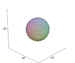
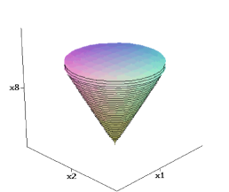
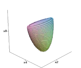
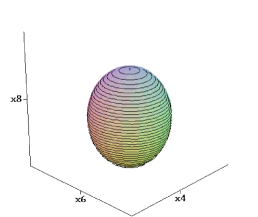
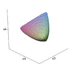
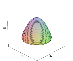
Figure 1: Some three-dimensional sections of the eight-dimensional set ${\mathbb{S}_{3}}$ of the statistical operators for a three-level quantum system. The adopted coordinate system is explained in § III.

We study data $D$ and prior knowledge $I$ of the following kind:

• The measurement data $D$ consist in a set of $N$ outcomes of $N$ instances of the same measurement performed on $N$ identically prepared systems. The measurement is represented by the extreme positive-operator-valued measure (i.e., non-degenerate ‘von Neumann measurement’) having three possible distinct outcomes $\{\text{`1'},\text{`2'},\text{`3'}\}$ represented by the eigenprojectors $\{\lvert 1\rangle\langle 1\rvert,\lvert 2\rangle\langle 2\rvert,\lvert 3\rangle\langle 3\rvert\}$. The data $D$ thus correspond to a triple of absolute frequencies $(N_{1},N_{2},N_{3})\eqqcolon\bar{N}$, with $N_{i}\geqslant 0$ and $\sum_{i}N_{i}=N$. We consider various such triples for small values of $N$, as well as for the limiting case of very large $N$.

• Two different kinds of prior knowledge $I$ are used. The first, $I_{\text{co}}$, is represented by a prior plausibility distribution

  $$p(\bm{\erho}\mathpunct{|}I_{\text{co}})\,\mathrm{d}\bm{\erho}=g_{\text{co}}(\bm{\erho})\,\mathrm{d}\bm{\erho}\propto\mathrm{d}\bm{\erho},$$ (2)

  which is constant in respect of the convex structure of the set of statistical operators, in the sense explained in §§ III and IV. The second, $I_{\text{ga}}$, is represented by a spherically symmetric, Gaussian-like prior distribution

  $$p(\bm{\erho}\mathpunct{|}I_{\text{ga}})\,\mathrm{d}\bm{\erho}=g_{\text{ga}}(\bm{\erho})\,\mathrm{d}\bm{\erho}\propto\exp\biggl{\{}-\frac{\operatorname{tr}[(\bm{\erho}-\lvert 2\rangle\langle 2\rvert)^{2}]}{s^{2}}\biggr{\}}\,\mathrm{d}\bm{\erho},$$ (3)

  centred on the statistical operator $\lvert 2\rangle\langle 2\rvert$, one of the projectors of the von Neumann measurement. This prior expresses some kind of knowledge that leads us to assign higher plausibility to regions in the vicinity of $\lvert 2\rangle\langle 2\rvert$.

To assign a statistical operator $\bm{\erho}_{D\land I}$ from these data and priors means to assign eight independent real coefficients of its matrix elements, or equivalently a vector of eight real parameters bijectively associated with them. These parameters, according to eq. (1b), must be computed by the integration of a function (actually two, the other being a normalisation factor) defined over the set of all statistical operators. Hence the function itself and the integration region can be expressed in terms of eight coordinates, corresponding to the parameters. The coordinate system should be chosen in such a way that both the function and the integration limits have a not too complex form. For these reasons we choose the parametrisation studied in particular by Kimura (Kimura, 2003). In this case the vectors of real parameters associated to a statistical operator is called a ‘Bloch vector’.

In such a coordinate system, six of the eight parameters can be calculated analytically and quite straightforwardly by symmetry arguments, for all absolute-frequency triples $\bar{N}$. The remaining two parameters have been numerically calculated for some triples $\bar{N}$ by a computer using quasi-Monte Carlo integration methods, suitable for high-dimensional problems. Further symmetry arguments yield the parameters for the remaining triples.

All these points as well as the results are discussed in the paper as follows: In § II we quickly present the reasoning leading to the statistical-operator-assignment formulae (1), and particularise the latter to our study. In § III Kimura’s parametrisation and the Bloch-vector set are introduced. The two prior distributions adopted are discussed in § IV. The calculation, by symmetry arguments and by numerical integration, of the Bloch vectors and of the corresponding statistical operators is presented in § V, for all data and priors. In § VI we offer some remarks on the incorporation into the formalism of uncertainties in the detection of outcomes. In § VII we discuss the form the assigned statistical operator takes in the limit of a very large number of measurements. Finally, the last section summarises and discusses the main points and results.

II Statistical-operator assignment

II.1 General case

This section provides a summary derivation of the formulae for statistical-operator assignment. For a more general derivation of analogous formulae valid for any kind of system (classical, quantum, or exotic), and for a discussion of some philosophical points involved, we refer the reader to (Porta Mana et al., 2006, 2007; Porta Mana, 2007a, b) and also (Mana, 2003, 2004).

There is a preparation scheme that produces quantum systems always in the same ‘condition’ — the same ‘state’. We do not know which this condition is, amongst a set of possible ones; although there may be some conditions in that set that are more plausible than others. Our knowledge $I$, in other words, is expressed by a plausibility distribution over these conditions. To each condition is associated a statistical operator; this encodes the plausibility distributions that we assign for all possible quantum measurements, given that that particular condition hold. Therefore we can and shall more simply speak in terms of statistical operators instead of the respective conditions. Note that this is, however, a metonymy, i.e. we are speaking about something (‘statistical operator’) although it is something else but related to it (‘condition’) that we really mean.

We thus have a plausibility distribution over some statistical operators. It can in full generality be written as

$$p(\bm{\erho}\mathpunct{|}I)\,\mathrm{d}\bm{\erho}=g(\bm{\erho})\,\mathrm{d}\bm{\erho},$$ (4)

defined over the whole set of statistical operators, denoted by $\mathbb{S}$. The function $g$ is a normalised positive generalised function. In this way the more general case is also accounted for in which the whole set of statistical operators $\mathbb{S}$ is involved: the case with a finite number of a priori possible statistical operators corresponds to a $g$ equal to a sum of appropriately weighted Dirac deltas.

Our ‘prior’ knowledge $I$ about the preparation can be represented by a unique statistical operator: Suppose we are to give the plausibility of the th outcome of an arbitrary measurement, represented by the positive-operator-valued measure $\{\bm{\evarEpsilon}\}$, performed on a system produced according to the preparation. Quantum mechanics dictates the plausibilities $p(\bm{\evarEpsilon}\mathpunct{|}\bm{\erho})=\operatorname{tr}(\bm{\evarEpsilon}\bm{\erho})$, and by the rules of plausibility theory we assign, conditional on $I$,

$$p(\bm{\evarEpsilon}\mathpunct{|}I)=\int_{\mathbb{S}}p(\bm{\evarEpsilon}\mathpunct{|}\bm{\erho})\,p(\bm{\erho}\mathpunct{|}I)\,\mathrm{d}\bm{\erho}=\int_{\mathbb{S}}\operatorname{tr}(\bm{\evarEpsilon}\bm{\erho})\,g(\bm{\erho})\,\mathrm{d}\bm{\erho},$$ (5)

or more compactly, by linearity of the trace,

$$\begin{split}p(\bm{\evarEpsilon}\mathpunct{|}I)&=\operatorname{tr}\bigl{[}\bm{\evarEpsilon}\smallint\bm{\erho}\,g(\bm{\erho})\,\mathrm{d}\bm{\erho}\bigr{]},\\ &=\operatorname{tr}(\bm{\evarEpsilon}\bm{\erho}_{I}),\end{split}$$ (6)

with the statistical operator $$\bm{\erho}_{I}$$ defined as

$$\bm{\erho}_{I}\coloneqq\int_{\mathbb{S}}\bm{\erho}\,p(\bm{\erho}\mathpunct{|}I)\,\mathrm{d}\bm{\erho}=\int_{\mathbb{S}}\bm{\erho}\,g(\bm{\erho})\,\mathrm{d}\bm{\erho}.$$ (7)

The prior knowledge $I$ can thus be compactly represented by, or “encoded in”, the statistical operator $\bm{\erho}_{I}$. Note how $\bm{\erho}_{I}$ appears naturally, without the need to invoke decision-theoretics arguments and concepts, like cost functions etc. Note also that the association between $I$ and $\bm{\erho}_{I}$ is by construction valid for generic knowledge $I$, be it “prior” or not.

The statistical operator $\bm{\erho}_{I}$ is a “disposable” object. As soon as we know the outcome of a measurement on a system produced according to our preparation, the plausibility distribution $p(\bm{\erho}\mathpunct{|}I)\,\mathrm{d}\bm{\erho}$ should be updated on the evidence of this new piece of data $D$, and thus we get a new statistical operator $\bm{\erho}_{I\land D}$. And so on. It is a fundamental characteristic of plausibility theory that this update can indifferently be performed with a piece of data at a time or all at once.

So suppose we come to know that $N$ measurements, represented by the $N$ positive-operator-valued measures $\{\bm{\evarEpsilon}^{(k)}\colon\emu=1,\dotsc,r_{k}\}$, $k=1,\dotsc,N$, are or have been performed on $N$ systems for which our knowledge $I$ holds. Note that some, even all, of the measurements (and therefore their positive-operator-valued measures) can be identical. The outcomes $i_{1},\dotsc,i_{k},\dotsc,i_{N}$ are or were obtained; this is our new data $D$. The plausibility for this to occur, according to the prior knowledge $I$, is given by a generalisation of expression (5):

$$p(D\mathpunct{|}I)\equiv p\bigl{(}\bm{\evarEpsilon}^{(1)}_{i_{1}},\dotsc,\bm{\evarEpsilon}^{(N)}_{i_{N}}\mathpunct{|}I\bigr{)}=\int_{\mathbb{S}}\Bigl{[}\operatorname*{\textstyle\prod}_{k=1}^{N}p\bigl{(}\bm{\evarEpsilon}^{(k)}_{i_{k}}\mathpunct{|}\bm{\erho}\bigr{)}\Bigr{]}\,p(\bm{\erho}\mathpunct{|}I)\,\mathrm{d}\bm{\erho}.$$ (8)

On the evidence of $D$ we can update the prior plausibility distribution $p(\bm{\erho}\mathpunct{|}I)\,\mathrm{d}\bm{\erho}$. By the rules of plausibility theory

$$\begin{split}p(\bm{\erho}\mathpunct{|}D\land I)\,\mathrm{d}\bm{\erho}&=\frac{p(D\mathpunct{|}\bm{\erho})\,p(\bm{\erho}\mathpunct{|}I)\,\mathrm{d}\bm{\erho}}{\int_{\mathbb{S}}p(D\mathpunct{|}\bm{\erho})\,p(\bm{\erho}\mathpunct{|}I)\,\mathrm{d}\bm{\erho}},\\ &=\frac{\Bigl{[}\operatorname*{\textstyle\prod}_{k}\operatorname{tr}\bigl{(}\bm{\evarEpsilon}^{(k)}_{i_{k}}\bm{\erho}\bigr{)}\Bigr{]}\,g(\bm{\erho})\,\mathrm{d}\bm{\erho}}{\int_{\mathbb{S}}\Bigl{[}\operatorname*{\textstyle\prod}_{k}\operatorname{tr}\bigl{(}\bm{\evarEpsilon}^{(k)}_{i_{k}}\bm{\erho}\bigr{)}\Bigr{]}\,g(\bm{\erho})\,\mathrm{d}\bm{\erho}}.\end{split}$$ (9)

The statistical operator encoding the joint knowledge $D\land I$ is thus, according to eq. (7) and using eq. (9),

$$\bm{\erho}_{D\land I}\coloneqq\int_{\mathbb{S}}\bm{\erho}\,p(\bm{\erho}\mathpunct{|}D\land I)\,\mathrm{d}\bm{\erho}=\frac{\int_{\mathbb{S}}\bm{\erho}\Bigl{[}\operatorname*{\textstyle\prod}_{k}\operatorname{tr}\bigl{(}\bm{\evarEpsilon}^{(k)}_{i_{k}}\bm{\erho}\bigr{)}\Bigr{]}\,g(\bm{\erho})\,\mathrm{d}\bm{\erho}}{\int_{\mathbb{S}}\Bigl{[}\operatorname*{\textstyle\prod}_{k}\operatorname{tr}\bigl{(}\bm{\evarEpsilon}^{(k)}_{i_{k}}\bm{\erho}\bigr{)}\Bigr{]}\,g(\bm{\erho})\,\mathrm{d}\bm{\erho}}.$$ (10)

II.2 Three-level case

So far everything has been quite general. Let us now consider the particular cases studied in this paper.

The preparation scheme concerns three-level quantum systems; the corresponding set of statistical operators will be denoted by ${\mathbb{S}_{3}}$. The $N$ measurements considered here are all instances of the same measurement, namely a non-degenerate projection-valued measurement (often called ‘von Neumann measurement’). Thus, for all $k=1,\dotsc,N$, $\{\bm{\evarEpsilon}^{(k)}\}=\{\bm{\evarEpsilon}\}\coloneqq\{\lvert 1\rangle\langle 1\rvert,\lvert 2\rangle\langle 2\rvert,\lvert 3\rangle\langle 3\rvert\}$. The projectors $\lvert 1\rangle\langle 1\rvert$, $\lvert 2\rangle\langle 2\rvert$, $\lvert 3\rangle\langle 3\rvert$ define an orthonormal basis in Hilbert space. All relevant operators will, quite naturally and advantageously, be expressed in this basis. We have for example that $\operatorname{tr}(\bm{\evarEpsilon}\bm{\erho})\equiv$, the th diagonal element of .

The data $D$ consist in the set of outcomes $\{i_{1},\dotsc,i_{N}\}$ of the $N$ measurements, where each $i_{k}$ is one of the three possible outcomes ‘1’, ‘2’, or ‘3’. The formula (10) for the statistical operator thus takes the form

$$\bm{\erho}_{D\land I}=\frac{\int_{{\mathbb{S}_{3}}}\bm{\erho}\,\Bigl{[}\operatorname*{\textstyle\prod}_{k=1}^{N}{}_{i_{k}i_{k}}\Bigr{]}\,g(\bm{\erho})\,\mathrm{d}\bm{\erho}}{\int_{{\mathbb{S}_{3}}}\Bigl{[}\operatorname*{\textstyle\prod}_{k=1}^{N}{}_{i_{k}i_{k}}\Bigr{]}\,g(\bm{\erho})\,\mathrm{d}\bm{\erho}},$$ (11)

with $i_{k}\in\{1,2,3\}$ for all $k$.

However, it is clear from the expressions in the integrals above that the exact order of the sequence of ‘1’s, ‘2’s, and ‘3’s is unimportant; only the absolute frequencies $(N_{1},N_{2},N_{3})$ of appearance of these three possible outcomes matter (naturally, $N_{i}\geqslant 0$ and ${\textstyle\sum}_{i}N_{i}=N$). We can thus rewrite the last equation as

$$\bm{\erho}_{D\land I}=\frac{\int_{\mathbb{S}_{3}}\bm{\erho}\,\Bigl{[}\operatorname*{\textstyle\prod}_{i=1}^{3}{}_{ii}^{N_{i}}\Bigr{]}\,g(\bm{\erho})\,\mathrm{d}\bm{\erho}}{\int_{\mathbb{S}_{3}}\Bigl{[}\operatorname*{\textstyle\prod}_{i=1}^{3}{}_{ii}^{N_{i}}\Bigr{]}\,g(\bm{\erho})\,\mathrm{d}\bm{\erho}},$$ (12)

with the convention, here and in the following, that ${}_{ii}^{N_{i}}\coloneqq 1$ whenever $N_{i}={}_{ii}=0$ (the reason is that the product originally is, to wit, restricted to the terms with $N_{i}>0$).

The discussion of the explicit form of the prior $g(\bm{\erho})\,\mathrm{d}\bm{\erho}$ is deferred to § IV. We shall first introduce on ${\mathbb{S}_{3}}$ a suitable coordinate system $(x_{1},\dotsc,x_{8})\equiv\bm{x}\in\mathbb{R}^{8}$ so as to explicitly calculate the integrals. This is done in the next section.

III Bloch vectors

In order to calculate the integrals required in the state-assignment formula (12) we put a suitable coordinate system on ${\mathbb{S}_{3}}$, so that they “translate” as integrals in $\mathbb{R}^{8}$. In differential-geometrical terms, we choose a particular chart on ${\mathbb{S}_{3}}$ considered as a differentiable manifold (Kobayashi and Nomizu, 1963; Boothby, 1975/1986; Choquet-Bruhat et al., 1977/1996; Marsden et al., 1983/2002; Curtis and Miller, 1985; Gallot et al., 1987; Kennington, 2001/2006).

There exists an ‘Euler angle’ parametrisation (Byrd, 1998; Byrd and Slater, 2001; Tilma and Sudarshan, 2002a, b) which maps ${\mathbb{S}_{3}}$ onto a rectangular region of $\mathbb{R}^{8}$ (modulo identification of some points). With this parametrisation the integration limits of our integrals become advantageously independent, but the integrands ($p(D\mathpunct{|}\bm{\erho})$ in particular) acquire too complex a form.

For the latter reason we choose, instead, the parametrisation studied by Byrd, Slater and Khaneja (Byrd and Slater, 2001; Byrd and Khaneja, 2003), Kimura (Kimura, 2003) (see also (Kimura and Kossakowski, 2005)), and Bölükbaşı and Dereli (Bölükbaşı and Dereli, 2006), amongst others. The functions to be integrated take simple polynomials or exponentials forms. The integration limits are no longer independent, though — in fact, they are given in an implicit form and will be accounted for by multiplying the integrands by a characteristic function.

We follow Kimura’s study Kimura (2003) here, departing from it on some definitions. All statistical operators of a $d$-level quantum system can be written in the following form Kimura (2003) (see also Byrd and Slater (2001); Byrd and Khaneja (2003); Kimura and Kossakowski (2005)):

$$\bm{\erho}=\bm{\erho}(\bm{x})=\frac{1}{d}\bm{I}_{d}+\frac{1}{2}\sum_{j=1}^{n}x_{j}\bm{\elambda}_{j},\quad(x_{1},\dotsc,x_{n})\equiv\bm{x}\in\mathbb{B}_{n}\subset\mathbb{R}^{n}.$$ (13)

where $n\equiv d^{2}-1$ is the dimension of $\mathbb{S}$, and $\mathbb{B}_{n}$ is a compact convex subset of $\mathbb{R}^{n}$. The operators $\{\bm{\elambda}_{j}\}$ satisfy (1) $\bm{\elambda}_{j}=\bm{\elambda}_{j}^{\dagger}$, (2) $\operatorname{tr}\bm{\elambda}_{j}=0$, (3) $\operatorname{tr}(\bm{\elambda}_{i}\bm{\elambda}_{j})=2{}_{ij}$. Together with the identity operator $\bm{I}_{d}$ they are generators of $\mathrm{SU}(d)$, and in respect of the Frobenius (Hilbert-Schmidt) inner product $\bm{\elambda}_{i}\cdot\bm{\elambda}_{j}\coloneqq\operatorname{tr}(\bm{\elambda}_{i}\bm{\elambda}_{j})$ (Hall, 2003/2004) they also constitute a complete orthogonal basis for the vector space of Hermitean operators on a $d$-dimensional Hilbert space. In fact, eq. (13) is simply the decomposition of the Hermitean operator in terms of such a basis. The vector $\bm{x}\equiv(x_{j})$ of coefficients in equation (13) is uniquely determined by :

$$x_{j}=x_{j}(\bm{\erho})=\operatorname{tr}(\bm{\elambda}_{j}\,\bm{\erho}).$$ (14)

The operators $\{\bm{\elambda}_{j}\}$, being Hermitean, can also be regarded as observables and then the equation above says that the $(x_{i})$ are the corresponding expectation values in the state : $x_{j}=\langle\bm{\elambda}_{j}\rangle_{\bm{\erho}}$ (Peres, 1995).

A systematic construction of generators of $\mathrm{SU}(d)$ which generalises the Pauli spin operators is known (see e.g. Hioe and Eberly (1981); Kimura (2003)). In particular, for $d=2$ they are the usual Pauli spin operators, and for $d=3$ they are the Gell-Mann matrices (see e.g. (Macfarlane et al., 1968)). In the eigenbasis $\{\lvert 1\rangle\langle 1\rvert,\lvert 2\rangle\langle 2\rvert,\lvert 3\rangle\langle 3\rvert\}$ of the von Neumann measurement $\{\bm{\evarEpsilon}\}$ introduced in the previous section these matrices assume the particular form

$$\begin{gathered}\bm{\elambda}_{1}=\begin{pmatrix}0&1&0\\ 1&0&0\\ 0&0&0\end{pmatrix},\quad\bm{\elambda}_{2}=\begin{pmatrix}0&-\mathrm{i}&0\\ \mathrm{i}&0&0\\ 0&0&0\end{pmatrix},\quad\bm{\elambda}_{3}=\begin{pmatrix}1&0&0\\ 0&0&0\\ 0&0&-1\end{pmatrix},\\ \bm{\elambda}_{4}=\begin{pmatrix}0&0&1\\ 0&0&0\\ 1&0&0\end{pmatrix},\quad\bm{\elambda}_{5}=\begin{pmatrix}0&0&-\mathrm{i}\\ 0&0&0\\ \mathrm{i}&0&0\end{pmatrix},\quad\bm{\elambda}_{6}=\begin{pmatrix}0&0&0\\ 0&0&1\\ 0&1&0\end{pmatrix},\\ \bm{\elambda}_{7}=\begin{pmatrix}0&0&0\\ 0&0&-\mathrm{i}\\ 0&\mathrm{i}&0\end{pmatrix},\quad\bm{\elambda}_{8}=\frac{1}{\sqrt{3}}\begin{pmatrix}1&0&0\\ 0&-2&0\\ 0&0&1\end{pmatrix}.\end{gathered}$$ (15a)

We see that our von Neumann measurement corresponds to the observable

$$\bm{\elambda}_{3}\equiv\lvert 1\rangle\langle 1\rvert+0\lvert 2\rangle\langle 2\rvert-\lvert 3\rangle\langle 3\rvert,$$ (15b)

the measurement outcomes being associated with the particular values $1$, $0$, and $-1$. These eigenvalues, however, are of no importance to us (they will be more relevant in the companion paper (Månsson et al., 2007)).

For a three-level system, and in the eigenbasis $\{\lvert 1\rangle\langle 1\rvert,\lvert 2\rangle\langle 2\rvert,\lvert 3\rangle\langle 3\rvert\}$, the operator in (13) can thus be written in matrix form as:

$$\bm{\erho}=\bm{\erho}(\bm{x})={}\\ \begin{pmatrix}\frac{1}{3}+\frac{1}{2}(x_{3}+\frac{1}{\sqrt{3}}x_{8})&\frac{1}{2}(x_{1}-\mathrm{i}x_{2})&\frac{1}{2}(x_{4}-\mathrm{i}x_{5})\\ \frac{1}{2}(x_{1}+\mathrm{i}x_{2})&\frac{1}{3}-\frac{1}{\sqrt{3}}x_{8}&\frac{1}{2}(x_{6}-\mathrm{i}x_{7})\\ \frac{1}{2}(x_{4}+\mathrm{i}x_{5})&\frac{1}{2}(x_{6}+\mathrm{i}x_{7})&\frac{1}{3}+\frac{1}{2}(-x_{3}+\frac{1}{\sqrt{3}}x_{8})\end{pmatrix}.$$ (16)

This matrix is Hermitean and has unit trace, so the remaining condition for it to be a statistical operator is that it be positive semi-definite (non-negative eigenvalues). This is equivalent to two conditions Kimura (2003) for the coefficients $\bm{x}$: with our definitions of the Gell-Mann matrices, the first is

$$\bm{x}^{2}\equiv{\textstyle\sum}_{k=1}^{8}x_{i}^{2}\leqslant\frac{4}{3},$$ (17a)

which limits $$\bm{x} 2/\sqrt{3}$$ to be inside or on a ball of radius ; the second is

$$8-18\bm{x}^{2}+27x_{3}\bigl{(}x_{1}^{2}+x_{2}^{2}-x_{6}^{2}-x_{7}^{2}\bigr{)}-6\sqrt{3}x_{8}^{3}+{}\\ 9\sqrt{3}x_{8}\bigl{[}2\bigl{(}x_{3}^{2}+x_{4}^{2}+x_{5}^{2}\bigr{)}-\bigl{(}x_{1}^{2}+x_{2}^{2}+x_{6}^{2}+x_{7}^{2}\bigr{)}\bigr{]}+{}\\ 54(x_{1}x_{4}x_{6}+x_{2}x_{4}x_{7}+x_{2}x_{5}x_{6}-x_{1}x_{5}x_{7})\geqslant 0.$$ (17b)

The set of all real vectors $\bm{x}$ satisfying conditions (17) is called the ‘Bloch-vector set’ ${\mathbb{B}_{8}}$ of the three-level system:

$${\mathbb{B}_{8}}\coloneqq\{\bm{x}\in\mathbb{R}^{8}\mathpunct{|}\text{\eqref{eq:bv} hold}\}.$$ (18)

Since there is a bijective correspondence between ${\mathbb{B}_{8}}$ and ${\mathbb{S}_{3}}$, we can parametrise the set of all statistical operators ${\mathbb{S}_{3}}$ by the set of all Bloch vectors.

Both ${\mathbb{S}_{3}}$ and ${\mathbb{B}_{8}}$ are convex sets (Valentine, 1964; Grünbaum, 1967/2003; Rockafellar, 1970; Alfsen, 1971; Brøndsted, 1983; Webster, 1994; Segal, 1947; Mackey, 1963; Mielnik, 1968, 1974; Bloore, 1976), and the maps

$${\mathbb{S}_{3}} \to{\mathbb{B}_{8}}\quad\text{by}\quad\bm{\erho}\mapsto\bm{x}(\bm{\erho})$$ (19)

given by (14), and its inverse

$${\mathbb{B}_{8}} \to{\mathbb{S}_{3}}\quad\text{by}\quad\bm{x}\mapsto\bm{\erho}(\bm{x})$$ (20)

given by (13) or (16) are convex isomorphisms, i.e. they preserve convex combinations:

$$\bm{x}({}^{\prime}\bm{\erho}^{\prime}+{}^{\prime\prime}\bm{\erho}^{\prime\prime})={}^{\prime}\bm{x}(\bm{\erho}^{\prime})+{}^{\prime\prime}\bm{x}(\bm{\erho}^{\prime\prime}),$$ (21)

$$\bm{\erho}({}^{\prime}\bm{x}^{\prime}+{}^{\prime\prime}\bm{x}^{\prime\prime})={}^{\prime}\bm{\erho}(\bm{x}^{\prime})+{}^{\prime\prime}\bm{\erho}(\bm{x}^{\prime\prime}),$$ (22)

with ${}^{\prime},{}^{\prime\prime}\geqslant 0$, ${}^{\prime}+{}^{\prime\prime}=1$. This fact will be relevant for the discussion of the prior distributions.

It is useful to introduce the characteristic function $\bm{x}\mapsto{}_{\mathbb{B}}(\bm{x})$ of the set ${\mathbb{B}_{8}}$:

$${}_{\mathbb{B}}(\bm{x})\coloneqq\begin{cases}1&\text{if $\bm{x}\in{\mathbb{B}_{8}}$, {i.e.}\ if\leavevmode\nobreak\ \eqref{eq:bv} hold},\\ 0&\text{if $\bm{x}\notin{\mathbb{B}_{8}}$, {i.e.}\ if\leavevmode\nobreak\ \eqref{eq:bv} do not hold},\end{cases}$$ (23)

and to consider the smallest eight-dimensional rectangular region (or ‘orthotope’ (Grünbaum, 1967/2003)) ${\mathbb{C}_{8}}$ containing ${\mathbb{B}_{8}}$. As shown in the appendix, ${\mathbb{C}_{8}}$ is

$${\mathbb{C}_{8}}\coloneqq\lclose-1,1\rclose^{7}\times\Bigl{\lclose}-\tfrac{2}{\sqrt{3}},\tfrac{1}{\sqrt{3}}\Bigr{\rclose}\supset{\mathbb{B}_{8}}.$$ (24)

The relations amongst ${\mathbb{S}_{3}}$, ${\mathbb{B}_{8}}$, and ${\mathbb{C}_{8}}$ are schematically illustrated in fig. 2. In fig. 1 we can see some three-dimensional sections (through the origin) of ${\mathbb{B}_{8}}$ — and thus of ${\mathbb{S}_{3}}$ as well, in the sense of their isomorphism.

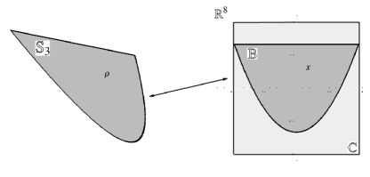
Figure 2: Schematic illustration of the relations amongst ${\mathbb{S}_{3}}$, ${\mathbb{B}_{8}}$, and ${\mathbb{C}_{8}}$.

We are almost ready to write the integrals of formula (12) in coordinate form, i.e. as integrals over $\mathbb{R}^{8}$. It only remains to specify the volume element $\mathrm{d}\bm{\erho}$ in coordinate form. What we shall do is in fact the opposite: we define $\mathrm{d}\bm{\erho}$ to be the volume element on ${\mathbb{S}_{3}}$ which in the coordinates $\bm{x}$ is simply $\mathrm{d}\bm{x}$. In differential-geometrical terms, $\mathrm{d}\bm{\erho}$ is the pull-back (Choquet-Bruhat et al., 1977/1996; Marsden et al., 1983/2002; Curtis and Miller, 1985; Gallot et al., 1987; Kennington, 2001/2006) of $\mathrm{d}\bm{x}$ induced by the map $\bm{\erho}\mapsto\bm{x}$:

$$\mathrm{d}\bm{\erho}\mapsto\mathrm{d}\bm{x}.$$ (25)

It is worth noting that this choice of volume element is not arbitrary, but rather quite natural. On any $n$-dimensional convex set $S$ we can define a volume element which is canonical in respect of $S$’s convex structure, as follows. Consider any convex isomorphism $c\colon S\to B$ between $S$ and some subset $B\subset\mathbb{R}^{n}$. Consider the volume element on $B$ defined by

$$\eomega\coloneqq\mathrm{d}\bm{y}/\smallint_{B}\mathrm{d}\bm{y},$$ (26)

where $\mathrm{d}\bm{y}$ is the canonical volume element on $\mathbb{R}^{n}$. The pull-back $c^{*}(\eomega)$ of onto $S$ then yields a volume element on the latter. It is easy to see that the volume element thus induced (1) does not depend on the particular isomorphism $c$ (and set $B$) chosen, since all such isomorphisms are related by affine coordinate changes ($\bm{y}\mapsto\bm{A}\bm{y}+\bm{b}$, with $\det\bm{A}\neq 0$, $\bm{b}\in\mathbb{R}^{n}$); (2) is invariant in respect of convex automorphisms of $S$; (3) assigns unit volume to $S$, as clear from eq. (26). These properties make this volume element canonical.

Since the parametrisation ${\mathbb{S}_{3}}\to{\mathbb{B}_{8}}$ is a convex isomorphism, we see that $\mathrm{d}\bm{\erho}$ as defined in (25) is the canonical volume element of ${\mathbb{S}_{3}}$ in respect of its convex structure.

We can finally write any integral over ${\mathbb{S}_{3}}$ in coordinate form. If $\bm{\erho}\mapsto f(\bm{\erho})$ is an integrable (possibly vector-valued) function over ${\mathbb{S}_{3}}$, its integral becomes

$$\int_{\mathbb{S}_{3}}f(\bm{\erho})\,\mathrm{d}\bm{\erho}\equiv\int_{\mathbb{C}_{8}}f[\bm{\erho}(\bm{x})]\,{}_{\mathbb{B}}(\bm{x})\,\mathrm{d}\bm{x}\equiv{}\\ \int_{-1}^{1}\mathrm{d}x_{1}\,\dotsi\int_{-1}^{1}\mathrm{d}x_{7}\int_{-\frac{2}{\sqrt{3}}}^{\frac{1}{\sqrt{3}}}\mathrm{d}x_{8}\,f[\bm{\erho}(\bm{x})]\,{}_{\mathbb{B}}(\bm{x}).$$ (27)

This form is especially suited to numerical integration by computer and we shall use it hereafter. We can thus rewrite the state-assignment formula (12) for $\bm{\erho}_{D\land I}$ as:

$$\bm{\erho}_{D\land I}=\frac{\int_{\mathbb{C}_{8}}\bm{\erho}(\bm{x})\,\Bigl{[}\operatorname*{\textstyle\prod}_{i=1}^{3}{}_{ii}(\bm{x})^{N_{i}}\Bigr{]}\,{}_{\mathbb{B}}(\bm{x})\,g(\bm{x})\,\mathrm{d}\bm{x}}{\int_{\mathbb{C}_{8}}\Bigl{[}\operatorname*{\textstyle\prod}_{i=1}^{3}{}_{ii}(\bm{x})^{N_{i}}\Bigr{]}\,{}_{\mathbb{B}}(\bm{x})\,g(\bm{x})\,\mathrm{d}\bm{x}}.$$ (28)

Expanding the $\bm{\erho}(\bm{x})$ inside the integrals using eq. (13) (equivalent to (16)) we further obtain

$$\bm{\erho}_{D\land I}=\frac{1}{3}\bm{I}_{3}+\frac{1}{2}\sum_{j=1}^{8}\frac{L_{j}(\bar{N},I)}{Z(\bar{N},I)}\bm{\elambda}_{j},$$ (29)

where

$$L_{j}(\bar{N},I) \coloneqq\int_{\mathbb{C}_{8}}x_{j}\,\Bigl{[}\operatorname*{\textstyle\prod}_{i=1}^{3}{}_{ii}(\bm{x})^{N_{i}}\Bigr{]}\,g(\bm{x})\,{}_{\mathbb{B}}(\bm{x})\,\mathrm{d}\bm{x},$$ (30a)

for $$j=1,\dotsc,8$$, and

$$Z(\bar{N},I) \coloneqq\int_{\mathbb{C}_{8}}\Bigl{[}\operatorname*{\textstyle\prod}_{i=1}^{3}{}_{ii}(\bm{x})^{N_{i}}\Bigr{]}\,g(\bm{x})\,{}_{\mathbb{B}}(\bm{x})\,\mathrm{d}\bm{x}.$$ (30b)

We shall omit the argument ‘$(\bar{N},I)$’ from both $L_{j}$ and $Z$ when it should be clear from the context.

It is now time to discuss the prior plausibility distributions adopted in our study.

IV Prior knowledge

The prior knowledge $I$ about the preparation is expressed as a prior plausibility distribution $p(\bm{\erho}\mathpunct{|}I)\,\mathrm{d}\bm{\erho}=g(\bm{\erho})\,\mathrm{d}\bm{\erho}$. The last expression can be interpreted, in measure-theoretic terms (Rudin, 1953/1976, 1970)(Choquet-Bruhat et al., 1977/1996, § I.D) (Fremlin, 2000/2004) (cf. also (Kolmogorov, 1933/1956; Doob, 1996)), as ‘$\emu(\mathrm{d}\bm{\erho})$’, where is a normalised measure; or it can be simply interpreted, as we do here, as the product of a generalised function $g$ and the volume element $\mathrm{d}\bm{\erho}$. The two points of view are not mutually exclusive of course, and these technical matters are only relatively important since ${\mathbb{S}_{3}}$ and the distributions we consider are quite well-behaved objects (and the simple Riemann integral suffices for our purposes).

We shall specify the plausibility distributions on ${\mathbb{S}_{3}}$ giving them directly in coordinate form on ${\mathbb{B}_{8}}$ (with an abuse of notation for $g$):

$$p(\bm{x}\mathpunct{|}I)\,\mathrm{d}\bm{x}=g(\bm{x})\,\mathrm{d}\bm{x}\coloneqq g[\bm{\erho}(\bm{x})]\,\mathrm{d}\bm{x}.$$ (31)

The first kind of prior knowledge considered in our study, $I_{\text{co}}$, has a constant density:

$$p(\bm{x}\mathpunct{|}I_{\text{co}})\,\mathrm{d}\bm{x}=g_{\text{co}}(\bm{x})\,\mathrm{d}\bm{x}\propto\mathrm{d}\bm{x},$$ (32)

the proportionality constant being given by the inverse of the volume of ${\mathbb{B}_{8}}$. This distribution hence corresponds to the canonical volume element (or the canonical measure) discussed in the previous section. Thus $I_{\text{co}}$ expresses somehow “vague” prior knowledge (although we do not necessarily maintain that it be “uninformative”). Fig. 3 shows the marginal density of the coordinates $x_{3}$ and $x_{8}$ for this prior. The state-assignment formula which makes use of this prior assumes the simplified form

$$\bm{\erho}_{D\land I_{\text{co}}}=\frac{\int_{\mathbb{C}_{8}}\bm{\erho}(\bm{x})\,\Bigl{[}\operatorname*{\textstyle\prod}_{i=1}^{3}{}_{ii}(\bm{x})^{N_{i}}\Bigr{]}\,{}_{\mathbb{B}}(\bm{x})\,\mathrm{d}\bm{x}}{\int_{\mathbb{C}_{8}}\Bigl{[}\operatorname*{\textstyle\prod}_{i=1}^{3}{}_{ii}(\bm{x})^{N_{i}}\Bigr{]}\,{}_{\mathbb{B}}(\bm{x})\,\mathrm{d}\bm{x}}.$$ (33)

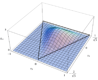
Figure 3: Graph of the constant prior’s marginal density $(x_{3},x_{8})\mapsto\smallint g_{\text{co}}\,\mathrm{d}x_{1}\,\mathrm{d}x_{2}\,\mathrm{d}x_{4}\,\mathrm{d}x_{5}\,\mathrm{d}x_{6}\,\mathrm{d}x_{7}$. The triangle represents the boundary of ${\mathbb{B}_{8}}$ in the $\bm{O}x_{3}x_{8}$ plane (see § V.2, and cf. figs. 5–9).

The second prior to be considered expresses somehow better knowledge $I_{\text{ga}}$ of the possible preparation. In coordinate form it is represented by the spherically symmetric Gaussian-like distribution

$$p(\bm{x}\mathpunct{|}I_{\text{ga}})\,\mathrm{d}\bm{x}=g_{\text{ga}}(\bm{x})\,\mathrm{d}\bm{x}\propto{}\\ \exp\Biggl{(}-\frac{\operatorname{tr}\bigl{\{}[\bm{\erho}(\bm{x})-\bm{\erho}(\hat{\bm{x}})]^{2}\bigr{\}}}{s^{2}}\Biggr{)}\,\mathrm{d}\bm{x}\equiv\exp\Biggl{[}\frac{(\bm{x}-\hat{\bm{x}})^{2}}{2s^{2}}\Biggr{]}\,\mathrm{d}\bm{x},$$ (34)

with

$$\hat{\bm{x}}\coloneqq(0,0,0,0,0,0,0,-2/\sqrt{3}),\quad\text{{i.e.},}\quad\bm{\erho}(\hat{\bm{x}})\equiv\lvert 2\rangle\langle 2\rvert,$$ (35)

$$s=\frac{1}{2\sqrt{2}}.$$

Regions in proximity of $\lvert 2\rangle\langle 2\rvert$ have greater plausibility, and the plausibility of other regions decreases as their “distance” $\{\operatorname{tr}[\bm{\erho}(\bm{x})-\bm{\erho}(\hat{\bm{x}})]^{2}\}^{1/2}\mathrel{\hat{=}}\lvert\bm{x}-\hat{\bm{x}}\rvert$ from $\lvert 2\rangle\langle 2\rvert$ increases. The parameter $s$ may be called the ‘breadth’ of the Gaussian-like function. The marginal density of the coordinates $x_{3}$ and $x_{8}$ for this prior is shown in fig. 4. The state-assignment formula with the prior knowledge $I_{\text{ga}}$ assumes the form

$$\bm{\erho}_{D\land I_{\text{ga}}}=\frac{\int_{\mathbb{C}_{8}}\bm{\erho}(\bm{x})\,\Bigl{[}\operatorname*{\textstyle\prod}_{i=1}^{3}{}_{ii}(\bm{x})^{N_{i}}\Bigr{]}\,\exp\Bigl{[}\frac{(\bm{x}-\hat{\bm{x}})^{2}}{2s^{2}}\Bigr{]}\,{}_{\mathbb{B}}(\bm{x})\,\mathrm{d}\bm{x}}{\int_{\mathbb{C}_{8}}\Bigl{[}\operatorname*{\textstyle\prod}_{i=1}^{3}{}_{ii}(\bm{x})^{N_{i}}\Bigr{]}\,\exp\Bigl{[}\frac{(\bm{x}-\hat{\bm{x}})^{2}}{2s^{2}}\Bigr{]}\,{}_{\mathbb{B}}(\bm{x})\,\mathrm{d}\bm{x}}.$$ (36)

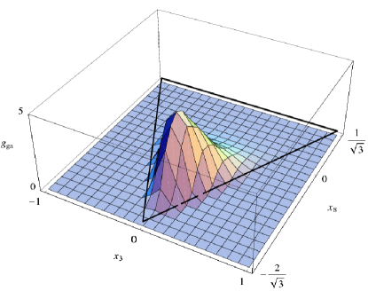
Figure 4: Graph of the Gaussian-like prior’s marginal density $(x_{3},x_{8})\mapsto\smallint g_{\text{ga}}\,\mathrm{d}x_{1}\,\mathrm{d}x_{2}\,\mathrm{d}x_{4}\,\mathrm{d}x_{5}\,\mathrm{d}x_{6}\,\mathrm{d}x_{7}$. The triangle represents the boundary of ${\mathbb{B}_{8}}$ in the $\bm{O}x_{3}x_{8}$ plane (see § V.2, and cf. figs. 5–9).

In the following the function $g(\bm{x})$ will generically stand for $g_{\text{co}}(\bm{x})$ or $g_{\text{ga}}(\bm{x})$.

V Explicit calculation of the assigned statistical operator

We shall now calculate the statistical operator given by (29), which means calculating the $L_{j}$ and $Z$ as given in (30a) and (30), for the triples of absolute frequencies

$$N =1\text{:} (1,0,0)\text{ and permutations thereof;}$$

$$N =2\text{:} (2,0,0),(1,1,0),\text{ and permutations;}$$

$$N =3\text{:} (3,0,0),(2,1,0),(1,1,1),\text{ and permutations;}$$

$$N =4,5,6,7\text{:} (0,N,0),$$

with the prior distribution $$g_{\text{co}}(\bm{x})\,\mathrm{d}\bm{x}$$; and the triples

$$N =1\text{:} (1,0,0),(0,1,0),(0,0,1);$$

with the Gaussian-like prior distribution $g_{\text{ga}}(\bm{x})\,\mathrm{d}\bm{x}$.

A combination of symmetries of ${\mathbb{B}_{8}}$ and numerical integration is used to compute $L_{j}$ and $Z$.

V.1 Deduction of some Bloch-vector parameters for some data via symmetry arguments

The coefficients $L_{j}$ for $j=1,2,4,5,6,7$ can be shown to vanish by symmetry arguments. Let us show that $L_{1}=0$ in particular. Consider

$$L_{1}\equiv\int_{\mathbb{C}_{8}}x_{1}\,\Bigl{[}\operatorname*{\textstyle\prod}_{i=1}^{3}{}_{ii}(\bm{x})^{N_{i}}\Bigr{]}\,g(\bm{x})\,{}_{\mathbb{B}}(\bm{x})\,\mathrm{d}\bm{x}.$$ (37)

The transformation

$$\bm{x}\equiv(x_{1},x_{2},x_{3},x_{4},x_{5},x_{6},x_{7},x_{8})\mapsto{}\\ \bm{x}^{\prime}\equiv(-x_{1},x_{2},x_{3},x_{4},x_{5},-x_{6},x_{7},-x_{8})$$ (38)

maps the domain ${\mathbb{C}_{8}}$ bijectively onto itself, and the absolute value of its Jacobian determinant is equal to unity. Under this transformation we have that

$$x^{\prime}_{1} =-x_{1},$$ (39a)

$$\bm{\erho}_{ii}(\bm{x}^{\prime}) =\bm{\erho}_{ii}(\bm{x})\quad i=1,2,3,$$ (39b)

$$g(\bm{x}^{\prime}) =g(\bm{x})\quad\text{(for both $g=g_{\text{co}},g_{\text{ga}}$)},$$ (39c)

$${}_{\mathbb{B}}(\bm{x}^{\prime}) ={}_{\mathbb{B}}(\bm{x}).$$ (39d)

Applying the formula for the change of variables (Schwartz, 1954; Lax, 1999) to (37), using the symmetries above, and renaming dummy integration variables we obtain

$$\begin{split}L_{1}&=\int_{\mathbb{C}_{8}}x_{1}\,\Bigl{[}\operatorname*{\textstyle\prod}_{i=1}^{3}{}_{ii}(\bm{x})^{N_{i}}\Bigr{]}\,g(\bm{x})\,{}_{\mathbb{B}}(\bm{x})\,\mathrm{d}\bm{x},\\ &=-\int_{\mathbb{C}_{8}}x_{1}\,\Bigl{[}\operatorname*{\textstyle\prod}_{i=1}^{3}{}_{ii}(\bm{x})^{N_{i}}\Bigr{]}\,g(\bm{x})\,{}_{\mathbb{B}}(\bm{x})\,\mathrm{d}\bm{x},\end{split}$$ (40)

$$\therefore L_{1} =0.$$ (41)

Similarly one can show that $L_{2}$, $L_{4}$, $L_{5}$, $L_{6}$, $L_{7}$ are all zero by changing the signs of the triplets $(x_{2},x_{5},x_{7})$, $(x_{1},x_{5},x_{6})$, $(x_{2},x_{4},x_{6})$, $(x_{2},x_{4},x_{6})$, $(x_{2},x_{5},x_{7})$, respectively.

The assigned statistical operator hence corresponds to the Bloch vector $(0,0,L_{3}/Z,0,0,0,0,L_{8}/Z)$, for all triples of absolute frequencies $\bar{N}$ and both kinds of prior knowledge. I.e. it has, in the eigenbasis $\{\lvert 1\rangle\langle 1\rvert,\lvert 2\rangle\langle 2\rvert,\lvert 3\rangle\langle 3\rvert\}$, the diagonal matrix form

$$\bm{\erho}_{D\land I}=\begin{pmatrix}\frac{1}{3}+\frac{L_{3}+L_{8}/\sqrt{3}}{2Z}&0&0\\ 0&\frac{1}{3}-\frac{L_{8}}{\sqrt{3}Z}&0\\ 0&0&\frac{1}{3}+\frac{-L_{3}+L_{8}/\sqrt{3}}{2Z}\end{pmatrix}$$ (42)

(note that $L_{3,8}$ and $Z$ still depend on $\bar{N}$ and $I$).

Two further changes of variables — both with unit Jacobian determinant and mapping ${\mathbb{B}_{8}}$ 1-1 onto itself — can be used to reduce the calculations for some absolute-frequency triples $(N_{1},N_{2},N_{3})$ to the calculation of other ones, with a reasoning similar to that of the preceding section.

The first is

$$\bm{x}\equiv(x_{1},x_{2},x_{3},x_{4},x_{5},x_{6},x_{7},x_{8})\mapsto{}\\ \bm{x}^{\prime}\equiv(x_{6},x_{7},-x_{3},x_{4},-x_{5},x_{1},x_{2},x_{8}),$$ (43)

under which, in particular,

$$\bm{\erho}_{11}(\bm{x}^{\prime})=\bm{\erho}_{33}(\bm{x}),\quad\bm{\erho}_{33}(\bm{x}^{\prime})=\bm{\erho}_{11}(\bm{x}),\quad\bm{\erho}_{22}(\bm{x}^{\prime})=\bm{\erho}_{22}(\bm{x}).$$ (44)

From eqs. (30) it follows that

$$L_{3}(N_{3},N_{2},N_{1}) =-L_{3}(N_{1},N_{2},N_{3}),$$ (45a)

$$L_{8}(N_{3},N_{2},N_{1}) =L_{8}(N_{1},N_{2},N_{3}),$$ (45b)

$$Z(N_{3},N_{2},N_{1}) =Z(N_{1},N_{2},N_{3}),$$ (45c)

for both prior distributions $g_{\text{co}}$ and $g_{\text{ga}}$.

The second change of variables is an anti-clockwise rotation of the plane $(x_{3},x_{8})$ by an angle $2\epi/3$ accompanied by permutations of the other coordinates:

$$(x_{1},x_{2},x_{3},x_{4},x_{5},x_{6},x_{7},x_{8})\mapsto{}\\ \biggl{(}x_{7},x_{6},-\frac{x_{3}+\sqrt{3}x_{8}}{2},x_{2},x_{1},x_{4},x_{5},\frac{\sqrt{3}x_{3}-x_{8}}{2}\Biggr{)},$$ (46)

under which, in particular,

$$\bm{\erho}_{11}(\bm{x}^{\prime})=\bm{\erho}_{22}(\bm{x}),\quad\bm{\erho}_{22}(\bm{x}^{\prime})=\bm{\erho}_{33}(\bm{x}),\quad\bm{\erho}_{33}(\bm{x}^{\prime})=\bm{\erho}_{11}(\bm{x}),$$ (47)

leading to

$$\begin{split}L_{3}[(N_{2},N_{3},N_{1}),I_{\text{co}}]&=-\frac{1}{2}L_{3}[(N_{1},N_{2},N_{3}),I_{\text{co}}]-{}\\ &\qquad\qquad\frac{\sqrt{3}}{2}L_{8}[(N_{1},N_{2},N_{3}),I_{\text{co}}],\end{split}$$ (48a)

$$\begin{split}L_{8}[(N_{2},N_{3},N_{1}),I_{\text{co}}]&=\frac{\sqrt{3}}{2}L_{3}[(N_{1},N_{2},N_{3}),I_{\text{co}}]-{}\\ &\qquad\qquad\frac{1}{2}L_{8}[(N_{1},N_{2},N_{3}),I_{\text{co}}],\end{split}$$ (48b)

$$Z[(N_{2},N_{3},N_{1}),I_{\text{co}}] =Z[(N_{1},N_{2},N_{3}),I_{\text{co}}].$$ (48c)

Note that the formulae from this transformation holds only for the constant prior $g_{\text{co}}$.

From (45) we see that, for both priors, $L_{3}$ vanishes for all triples of the form $(n,N-2n,n)$ for some positive integer $n\leqslant N/2$, in particular for $(0,N,0)$ and $(n,n,n)$. In the last case $L_{8}=0$ as well — though only for the constant prior $g_{\text{co}}$ —, as can be deduced from (45) and (48).

In the case of the prior knowledge $I_{\text{co}}$, it is easy to realise that, repeatedly applying the two transformations above, one can derive the values of $L_{3}$, $L_{8}$, and $Z$ for all triples $(N_{1},N_{2},N_{2})$ from the values for the triples with $N_{2}\geqslant N_{1}\geqslant N_{3}$ only.

V.2 Numerical calculation for the remaining cases

No other symmetry arguments seem available to derive $L_{3}$, $L_{8}$, and $Z$ for the remaining cases. In fact $L_{3}$, $L_{8}$ are in general non-zero ($Z$ can never vanish, its integrand being positive and never identically naught). It is very difficult — impossible perhaps? — to calculate the corresponding integrals analytically because of the complicated shape of ${\mathbb{B}_{8}}$. Therefore we have resorted to numerical integration, using the quasi-Monte Carlo integration algorithms provided by Mathematica 5.2.

The resulting Bloch vectors for the constant prior $g_{\text{co}}\,\mathrm{d}\bm{x}$ are shown for $N=1,2,3$ in figs. 5, 6, and 7 respectively. We have included in fig. 5 the case $N=0$ — i.e., no data — corresponding to the statistical operator $\bm{\erho}_{I_{\text{co}}}$ that encodes the prior knowledge $I_{\text{co}}$. In fig. 8 we have plotted the Bloch vectors corresponding to triples of the form $(N_{1},N_{2},N_{3})=(0,0,N)$ for $N=1,\dotsc,7$.

The cases $N=0$ and $N=1$ for the Gaussian-like prior $g_{\text{ga}}\,\mathrm{d}\bm{x}$ are shown in fig. 9. The case $N=0$ corresponds to the statistical operator $\bm{\erho}_{I_{\text{ga}}}$ encoding the prior knowledge $I_{\text{ga}}$.

The large triangle in the figures is the two-dimensional section of the set ${\mathbb{B}_{8}}$ along the plane $\bm{O}x_{3}x_{8}$. It can, of course, also be considered as a section of the set of statistical operators ${\mathbb{S}_{3}}$. This section contains the eigenprojectors $\lvert 1\rangle\langle 1\rvert$, $\lvert 2\rangle\langle 2\rvert$, $\lvert 3\rangle\langle 3\rvert$, which are the vertices of the triangle, as indicated. The assigned statistical operators, for all data and priors considered in this study, also lie on this triangle since they are mixtures of the eigenprojectors, as we found in § V.1, eq. (42). They are represented by points labelled with the respective data triples. The points have planar coordinates $\bigl{(}L_{3}(\bar{N},I)/Z(\bar{N},I),L_{8}(\bar{N},I)/Z(\bar{N},I)\bigr{)}$.

The numerical-integration uncertainties ₃ and ₈, for $L_{3}/Z$ and $L_{8}/Z$ respectively, specified in the figures’ legends, vary from $\pm 0.0025$ for the triplets with $N=2$ to $\pm 0.015$ for various other triplets. Numerical integration has also been performed for those quantities that can be determined analytically (§ V.1) — like $L_{3}(0,N,0)/Z(0,N,0)$ e.g. —, and the numerical results agree, within the uncertainties, with the analytical ones.

A trade-off between, on the one hand, calculation time and, on the other, accuracy of the result was necessary. The accuracy parameters to be inputted onto the integration routine were determined by previous rough numerical estimations of the results; in some cases an iterative process of this kind was adopted. The calculation of the statistical operator for a given triple of absolute frequencies $\bar{N}$ took from three to one hundred minutes, depending on the accuracy required and the complexity of the integrands.

$I_{\text{co}}$, $N=0$ (no data): $\bm{\erho}_{(000),I_{\text{co}}}=\begin{pmatrix}1/3&0&0\\ 0&1/3&0\\ 0&0&1/3\end{pmatrix}$ NB: This statistical operator encodes the prior knowledge $I_{\text{co}}$ $I_{\text{co}}$, $N=1$: $\bm{\erho}_{(010),I_{\text{co}}}=\begin{pmatrix}0.300\pm 0.001&0&0\\ 0&0.399\pm 0.003&0\\ 0&0&0.300\pm 0.001\end{pmatrix}$ cases $(100)$ and $(001)$ obtained by permutation $I_{\text{co}}$, $N=2$: $\bm{\erho}_{(020),I_{\text{co}}}=\begin{pmatrix}0.2735\pm 0.0007&0&0\\ 0&0.453\pm 0.001&0\\ 0&0&0.2735\pm 0.0007\end{pmatrix}$ $\bm{\erho}_{(101),I_{\text{co}}}=\begin{pmatrix}0.3642\pm 0.0007&0&0\\ 0&0.272\pm 0.001&0\\ 0&0&0.3642\pm 0.0007\end{pmatrix}$ other cases obtained by permutation $I_{\text{co}}$, $N=3$: $\bm{\erho}_{(030),I_{\text{co}}}=\begin{pmatrix}0.249\pm 0.001&0&0\\ 0&0.502\pm 0.003&0\\ 0&0&0.249\pm 0.001\end{pmatrix}$ $\bm{\erho}_{(021),I_{\text{co}}}=\begin{pmatrix}0.333\pm 0.004&0&0\\ 0&0.418\pm 0.003&0\\ 0&0&0.249\pm 0.004\end{pmatrix}$ $\bm{\erho}_{(111),I_{\text{co}}}=\begin{pmatrix}1/3&0&0\\ 0&1/3&0\\ 0&0&1/3\end{pmatrix}$ other cases obtained by permutation $I_{\text{co}}$, $N=4$: $\bm{\erho}_{(040),I_{\text{co}}}=\begin{pmatrix}0.230\pm 0.004&0&0\\ 0&0.541\pm 0.009&0\\ 0&0&0.230\pm 0.004\end{pmatrix}$ cases $(400)$ and $(004)$ obtained by permutation

$I_{\text{co}}$, $N=5$: $\bm{\erho}_{(050),I_{\text{co}}}=\begin{pmatrix}0.215\pm 0.004&0&0\\ 0&0.571\pm 0.009&0\\ 0&0&0.215\pm 0.004\end{pmatrix}$ cases $(500)$ and $(005)$ obtained by permutation $I_{\text{co}}$, $N=6$: $\bm{\erho}_{(060),I_{\text{co}}}=\begin{pmatrix}0.201\pm 0.004&0&0\\ 0&0.598\pm 0.009&0\\ 0&0&0.201\pm 0.004\end{pmatrix}$ cases $(600)$ and $(006)$ obtained by permutation $I_{\text{co}}$, $N=7$: $\bm{\erho}_{(070),I_{\text{co}}}=\begin{pmatrix}0.191\pm 0.004&0&0\\ 0&0.619\pm 0.009&0\\ 0&0&0.191\pm 0.004\end{pmatrix}$ cases $(700)$ and $(007)$ obtained by permutation $I_{\text{ga}}$, $N=0$ (no data): $\bm{\erho}_{(000),I_{\text{ga}}}=\begin{pmatrix}0.195\pm 0.004&0&0\\ 0&0.609\pm 0.009&0\\ 0&0&0.195\pm 0.004\end{pmatrix}$ NB: This statistical operator encodes the prior knowledge $I_{\text{ga}}$ $I_{\text{ga}}$, $N=1$: $\bm{\erho}_{(010),I_{\text{ga}}}=\begin{pmatrix}0.180\pm 0.004&0&0\\ 0&0.640\pm 0.009&0\\ 0&0&0.180\pm 0.004\end{pmatrix}$ $\bm{\erho}_{(001),I_{\text{ga}}}=\begin{pmatrix}0.239\pm 0.006&0&0\\ 0&0.575\pm 0.009&0\\ 0&0&0.186\pm 0.006\end{pmatrix}$ $\bm{\erho}_{(100),I_{\text{ga}}}=\begin{pmatrix}0.186\pm 0.006&0&0\\ 0&0.575\pm 0.009&0\\ 0&0&0.239\pm 0.006\end{pmatrix}$ Note that only two of the three uncertainties of the diagonal elements are independent; see § V.2. This has been computed from the average of the cases $(021)$ and $(120)$ (appropriately permuted).

Table 1: Statistical operators assigned for the various absolute-frequency data and priors considered in this study. Cf. figs. 5–9.

The statistical operators encoding the various kinds of data and prior knowledge are given in explicit form in table 1. Note that the uncertainties for the statistical operators should be written as ${}_{3}\bm{\elambda}_{3}/2+{}_{8}\bm{\elambda}_{8}/2$ (cf. eq. (29)); however, we adopted a more compact notation in the table (see footnote a there).

The results for $N=2$ and $N=3$ show an intriguing feature, immediately apparent in figs. 6 and 7: the computed Bloch vectors seem to maintain the convex structure of the respective data. What we mean is the following. For given $N$, the set of possible triples of absolute frequencies $(N_{1},N_{2},N_{3})$ has a natural convex structure with the extreme points $(N,0,0)$, $(0,N,0)$, and $(0,0,N)$:

$$(N_{1},N_{2},N_{3})\equiv(f_{1}N,f_{2}N,f_{3}N)={}\\ f_{1}(N,0,0)+f_{2}(0,N,0)+f_{3}(0,0,N),$$ (49)

where we have introduced the relative frequencies $f_{i}\coloneqq N_{i}/N$. Denote the Bloch vector corresponding to the triple $(N_{1},N_{2},N_{3})\equiv(f_{1}N,f_{2}N,f_{3}N)$ by

$$\bm{v}(N_{1},N_{2},N_{3})\coloneqq{}\\ \bigl{(}0,0,L_{3}(\bar{N},I_{\text{co}})/Z(\bar{N},I_{\text{co}}),0,0,0,0,L_{8}(\bar{N},I_{\text{co}})/Z(\bar{N},I_{\text{co}})\bigr{)}.$$ (50)

These Bloch vectors (and hence the statistical operators) seem, from figs. 6 and 7, to respect the same convex combinations as their respective triples:

$$\bm{v}(f_{1}N,f_{2}N,f_{3}N)\approx f_{1}\bm{v}(N,0,0)+f_{2}\bm{v}(0,N,0)+f_{3}\bm{v}(0,0,N).$$ (51)

In terms of the integrals (30) defining $L_{3}$, $L_{8}$, $Z$, and using (16) or (42), the seeming equation above becomes

$$\frac{\int_{\mathbb{B}_{8}}x_{j}\,\Bigl{(}\frac{1}{3}+\frac{x_{3}}{2}+\frac{x_{8}}{2\sqrt{3}}\Bigr{)}^{f_{1}N}\,\Bigl{(}\frac{1}{3}-\frac{x_{8}}{\sqrt{3}}\Bigr{)}^{f_{2}N}\,\Bigl{(}\frac{1}{3}-\frac{x_{3}}{2}+\frac{x_{8}}{2\sqrt{3}}\Bigr{)}^{f_{3}N}\,\mathrm{d}\bm{x}}{\int_{\mathbb{B}_{8}}\Bigl{(}\frac{1}{3}+\frac{x_{3}}{2}+\frac{x_{8}}{2\sqrt{3}}\Bigr{)}^{f_{1}N}\,\Bigl{(}\frac{1}{3}-\frac{x_{8}}{\sqrt{3}}\Bigr{)}^{f_{2}N}\,\Bigl{(}\frac{1}{3}-\frac{x_{3}}{2}+\frac{x_{8}}{2\sqrt{3}}\Bigr{)}^{f_{3}N}\,\mathrm{d}\bm{x}}\approx{}\\ f_{1}\frac{\int_{\mathbb{B}_{8}}x_{j}\,\Bigl{(}\frac{1}{3}+\frac{x_{3}}{2}+\frac{x_{8}}{2\sqrt{3}}\Bigr{)}^{N}\,\mathrm{d}\bm{x}}{\int_{\mathbb{B}_{8}}\Bigl{(}\frac{1}{3}+\frac{x_{3}}{2}+\frac{x_{8}}{2\sqrt{3}}\Bigr{)}^{N}\,\mathrm{d}\bm{x}}+f_{2}\frac{\int_{\mathbb{B}_{8}}x_{j}\,\Bigl{(}\frac{1}{3}-\frac{x_{8}}{\sqrt{3}}\Bigr{)}^{N}\,\mathrm{d}\bm{x}}{\int_{\mathbb{B}_{8}}\Bigl{(}\frac{1}{3}-\frac{x_{8}}{\sqrt{3}}\Bigr{)}^{N}\,\mathrm{d}\bm{x}}+f_{3}\frac{\int_{\mathbb{B}_{8}}x_{j}\,\Bigl{(}\frac{1}{3}-\frac{x_{3}}{2}+\frac{x_{8}}{2\sqrt{3}}\Bigr{)}^{N}\,\mathrm{d}\bm{x}}{\int_{\mathbb{B}_{8}}\Bigl{(}\frac{1}{3}-\frac{x_{3}}{2}+\frac{x_{8}}{2\sqrt{3}}\Bigr{)}^{N}\,\mathrm{d}\bm{x}},\quad j=3,8,$$ (52)

a remarkable expression. Does it hold exactly? We have not tried to prove or disprove its analytical validity, but it surely deserves further investigation. [Post scriptum: Slater, using cylindrical algebraic decomposition (Arnon et al., 1984a, b; Jirstrand, 1995) and a parametrisation by Bloore (cf. Slater, 2007), has confirmed that eq. (52) holds exactly. In fact, he has remarked that the some of the integrals, here numerically calculated, can be solved analytically by his approach.]

VI Taking account of the uncertainties in the detection of outcomes

Uncertainties are normally to be found in one’s measurement data, and need to be taken into account in the state-assignment procedure. For frequency data the uncertainty can stem from a combination of “over-counting”, i.e. the registration (because of background noise e.g.) of some events as outcomes when there are in fact none, and “under-counting”, i.e. the failure (because of detector limitations, e.g.) to register some outcomes.

Let us model the measurement-data uncertainty as follows, for definiteness. We say that the plausibility of registering the “event” ‘$i$’ when the outcome ‘’ is obtained is

$$\operatorname{P}(\text{`$i$'}\mathpunct{|}\text{`$\emu$'}\land I)=h(i\mathpunct{|}\emu).$$ (53)

The event ‘$i$’ belongs to some given set that may include such events as e.g. the ‘null’, no-detection event; the number of events need not be the same as the number of outcomes. The model formalised in the equation above suffices in many cases. Other models could take into account, e.g. “non-local” or memory effects, so that the plausibility of an event could depend on a set of previous or simultaneous outcomes. We thus definitely enter the realm of communication theory (Shannon, 1948, 1949; Middleton, 1960; Csiszár and Körner, 1981; Cover and Thomas, 1991) (see also (Helstrom, 1967, 1976)).

Given the preparation represented by the statistical operator , and the positive-operator-valued measure $\{\bm{\evarEpsilon}\}$ representing the measurement with outcomes $\{\text{`$\emu$'}\}$, the plausibility of registering the event ‘$i$’ in a measurement instance is, by the rules of plausibility theory,

$$p(i\mathpunct{|}\bm{\erho})={\textstyle\sum}p(i\mathpunct{|}\emu)\,p(\emu\mathpunct{|}\bm{\erho})={\textstyle\sum}h(i\mathpunct{|}\emu)\,\operatorname{tr}(\bm{\evarEpsilon}\bm{\erho}).$$ (54)

This marginalisation could be carried over to the state-assignment formulae already discussed in § II, and the formulae thus obtained would take into account the outcome-registration uncertainties.

However, it is much simpler to introduce a new positive-operator-valued measure $\{\bm{\evarDelta}_{i}\}$ defined by

$$\bm{\evarDelta}_{i}\coloneqq{\textstyle\sum}h(i\mathpunct{|}\emu)\bm{\evarEpsilon},$$ (55)

so that the plausibilities $p(i\mathpunct{|}\bm{\erho})$ in eq. (54) can be written, by the linearity of the trace,

$$p(i\mathpunct{|}\bm{\erho})=\operatorname{tr}(\bm{\evarDelta}_{i}\bm{\erho}).$$ (56)

In the state assignment we can simply use the new positive-operator-valued measure, which includes the outcome-registration uncertainties, in place of the old one. The last procedure is also more in the spirit of quantum mechanics: it is analogous to the use of the statistical operator $p_{1}\bm{\erho}_{1}+p_{2}\bm{\erho}_{2}$ when we are unsure (with plausibilities $p_{1}$ and $p_{2}$) about whether $\bm{\erho}_{1}$ or $\bm{\erho}_{2}$ holds. I.e., we can “mix” positive-operator-valued-measure elements just like we mix statistical operators. In fact, we could even mix, with a similar procedure, whole positive-operator-valued measures — a procedure which would represent the fact that there are uncertainties in the identification not only of the outcomes, but of the whole measurement procedure as well. See Peres’ partially related discussion (Peres, 2003).

VII Large-$N$ limit

VII.1 General case

Let us briefly consider the case of data with very large $N$. We summarise some results obtained in (Porta Mana, 2007b). Mathematically we want to see what form the state-assignment formulae take in the limit $N\to\infty$. Consider a sequence of data sets $\{D_{N}\}_{N=1}^{\infty}$. Each $D_{N}$ consists in some knowledge about the outcomes of $N$ instances of the same measurement. The latter is represented by the positive-operator-valued measure $\{\bm{\evarEpsilon}_{i}\}$. The plausibility distribution for the outcomes, given the preparation , is

$$\bm{q}(\bm{\erho})\coloneqq\bigl{(}q_{i}(\bm{\erho})\bigr{)}\quad\text{with}\quad q_{i}(\bm{\erho})=\operatorname{tr}(\bm{\evarEpsilon}_{i}\bm{\erho}).$$ (57)

Let us consider more precisely the general situation in which each data set $D_{N}$ consists in the knowledge that the relative frequencies $\bm{f}\equiv(f_{i})\coloneqq(N_{i}/N)$ lie in a region _N (with non-empty interior and whose boundary has measure zero in respect of the prior plausibility measure). Such kind of data arise when the registration of measurement outcomes is affected by uncertainties and is moreover “coarse-grained” for practical purposes, so that not precise frequencies are obtained but rather a region — like _N — of possible ones.

For each data set we then have a resulting posterior distribution for the statistical operators,

$$p(\bm{\erho}\mathpunct{|}D_{N}\land I)\,\mathrm{d}\bm{\erho}=p[\bm{\erho}\mathpunct{|}(\bm{f}\in{}_{N})\land I]\,\mathrm{d}\bm{\erho}={}\\ \frac{p(\bm{f}\in{}_{N}\mathpunct{|}\bm{\erho})\,p(\bm{\erho}\mathpunct{|}I)\,\mathrm{d}\bm{\erho}}{\int_{\mathbb{S}}p(\bm{f}\in{}_{N}\mathpunct{|}\bm{\erho})\,p(\bm{\erho}\mathpunct{|}I)\,\mathrm{d}\bm{\erho}}.$$ (58)

and an associated statistical operator $\bm{\erho}_{D_{N}\land I}\coloneqq\smallint\bm{\erho}\,p(\bm{\erho}\mathpunct{|}D_{N}\land I)\,\mathrm{d}\bm{\erho}$.

Assume that the sequence $\{{}_{N}\}_{N=1}^{\infty}$ of such frequency regions converges (in a topological sense specified in (Porta Mana, 2007b)) to a region _∞ (also with non-empty interior and with boundary of measure zero). We shall see later what happens when such a region shrinks to a single point, i.e. when the uncertainties becomes smaller and smaller. In (Porta Mana, 2007b) it is shown, using some theorems in Csiszár (Csiszár, 1984) and Csiszár and Shields (Csiszár and Shields, 2004), that

$$p(\bm{\erho}\mathpunct{|}D_{N}\land I)\,\mathrm{d}\bm{\erho}\propto\begin{cases}0,&\text{if $\bm{q}(\bm{\erho})\not\in{{}_{\infty}}$},\\ p(\bm{\erho}\mathpunct{|}I)\,\mathrm{d}\bm{\erho},&\text{if $\bm{q}(\bm{\erho})\in{{}_{\infty}}$},\end{cases}\\ \text{as $N\to\infty$}.$$ (59)

In other words: as the number of measurements becomes large, the plausibility of the statistical operators that encode a plausibility distribution not equal to one of the measured frequencies vanishes, so that the whole plausibility gets concentrated on the statistical operators encoding plausibility distributions equal to the possible frequencies. This is an intuitively satisfying result. The data single out a set of statistical operators, and these are then given weight according to the prior $p(\bm{\erho}\mathpunct{|}I)\,\mathrm{d}\bm{\erho}$, specified by us.

If _∞ degenerates into a single frequency value $\bm{f}^{*}$, the expression above becomes, as shown in (Porta Mana, 2007b),

$$p[\bm{\erho}\mathpunct{|}(\bm{f}=\bm{f}^{*})\land I]\,\mathrm{d}\bm{\erho}\propto p(\bm{\erho}\mathpunct{|}I)\,\edeltaup[\bm{q}(\bm{\erho})-\bm{f}^{*}]\,\mathrm{d}\bm{\erho},$$ (60)

which was also intuitively expected.

Note that if the prior density vanishes for such statistical operators as are singled out by the data, then the equations above become meaningless (no normalisation is possible), revealing a contradiction between the prior knowledge and the measurement data.

VII.2 Present case

In the case of our study, the derivation above shows that, as $N\to\infty$ and the triple of relative frequencies $\bm{f}\equiv(f_{1},f_{2},f_{3})\coloneqq(N_{1},N_{2},N_{3})/N$ tends to some value $\bm{f}^{*}$, the diagonal elements of the assigned statistical operator $\bm{\erho}_{D_{N}\land I}$ tend to

$$p(i\mathpunct{|}\bm{\erho}_{D_{N}\land I})\equiv(\bm{\erho}_{D_{N}\land I})_{ii}\to f^{*}_{i}\quad\text{as $N\to\infty$}.$$ (61)

Combining this with the results of § V.1 concerning the off-diagonal elements, we find that the assigned statistical operator has in the limit the form

$$\bm{\erho}_{D_{\infty}\land I}=\begin{pmatrix}f^{*}_{1}&0&0\\ 0&f^{*}_{2}&0\\ 0&0&f^{*}_{3}\end{pmatrix},$$ (62)

for both studied priors. This is again an expected result. Only the diagonal elements of the statistical operator are affected by the data, and as the data amount increases it overwhelms the prior information affecting the diagonal elements. Both priors are moreover symmetric in respect of the off-diagonal elements, that get thus a vanishing average.

VIII Discussion and conclusions

Bayesian quantum-state assignment techniques have been studied for some time now but, as far as we know, never been applied to the whole set of statistical operators of systems with more than two levels. And they have never been used for state assignment in real cases. In this study we have applied such methods to a three-level system, showing that the numerical implementation is possible and simple in principle. This paper should therefore not only be of theoretical interest but also be of use to experimentalists involved in state estimation. The time required to obtain the numerical results was relatively short in this three-level case, which involved an eight-dimensional integration. Application to higher-level systems should also be feasible, if one considers that integrals involving hundreds of dimensions are computed in financial, particle-physics, and image-processing problems (see e.g. the (somewhat dated) refs. (James, 1980; Stewart, 1983; LaValle et al., 1997; Sloan and Woźniakowski, 1998; Novak, 2000)).

Bayesian methods always take into account prior knowledge. We have given examples of state-assignment in the case of “vague” prior knowledge, as well as in the case of a kind of somehow better knowledge assigning higher plausibility to statistical operators in the vicinity of a given pure one. A comparison of the resulting statistical operators for the same kind of data is quickly obtained by looking at figs. 5 and 9 (or at the respective statistical operators in table 1). It is clear that when the available amount of data is small (as is the case in those figures, which concern data with no or only one measurement outcome), prior knowledge is very relevant. Any practised experimentalist usually has some kinds of prior knowledge in many experimental situations, which arise from past experience with similar situations. With some practice in “translating” these kinds of prior knowledge into distribution functions, one could employ small amounts of data in the most efficient way.

The generalisation of the present study to data involving different kinds of measurement is straightforward. Of course, in the general case one has to numerically determine a greater number of parameters (the $L_{j}$) and therefore compute a greater number of integrals. It would also be interesting to look at the results for other kinds of priors, in particular “special” priors like the Bures one (Slater, 1999; Byrd and Slater, 2001; Slater, 2001a, b; Sommers and Życzkowski, 2003). We found a particular non-trivial numerical relation, eq. (52), between the results obtained for the constant prior; it would be interesting to know whether it holds exactly.

In the next paper (Månsson et al., 2007) we shall give examples of numerical quantum-state assignment for data consisting in average values instead of absolute frequencies; and besides the two priors considered here we shall employ another prior studied by Slater (Slater, 1995).

Appendix A Determination of ${\mathbb{C}_{8}}$

Any hyperplane tangent to (supporting) a convex set must touch the latter on at least an extreme point (Valentine, 1964; Grünbaum, 1967/2003; Rockafellar, 1970; McMullen and Shephard, 1971; Brøndsted, 1983; Webster, 1994). To determine the hyper-sides of the minimal hyper-box ${\mathbb{C}_{8}}$ containing ${\mathbb{B}_{8}}$ we need therefore consider only the maximal points of the latter — i.e., the pure states.

A generic ray of a three-dimensional complex Hilbert space can be written as

$$\lvert\ephi\rangle=a\,\lvert 1\rangle+\mathrm{e}^{-\mathrm{i}\ebeta}b\,\lvert 2\rangle+\mathrm{e}^{-\mathrm{i}\egamma}c\,\lvert 3\rangle,$$ (63)

with

$$0\leqslant\ebeta,\egamma\leqslant 2\epiup,\qquad a,b,c\geqslant 0,\quad a^{2}+b^{2}+c^{2}=1;$$ (64)

note that any two of the parameters $a$, $b$, $c$ can be chosen independently in the range $\lclose 0,1\rclose$. The corresponding pure statistical operator is

$$\lvert\ephi\rangle\langle\ephi\rvert=\begin{pmatrix}a^{2}&\mathrm{e}^{-\mathrm{i}\ebeta}ab&\mathrm{e}^{-\mathrm{i}\egamma}ac\\ \mathrm{e}^{\mathrm{i}\ebeta}ab&b^{2}&\mathrm{e}^{-\mathrm{i}(\ebeta-\egamma)}bc\\ \mathrm{e}^{\mathrm{i}\egamma}ac&\mathrm{e}^{\mathrm{i}(\ebeta-\egamma)}bc&c^{2}\end{pmatrix}.$$ (65)

All pure states have this form, with the parameters in the ranges (64). Equating this expression with the one in terms of the Bloch-vector components $(x_{i})$, eq. (16), we obtain after some algebraic manipulation a parametric expression for the Bloch vectors of the pure states:

$$x_{1} =2ab\cos\ebeta, x_{2} =2ab\sin\ebeta,$$ (66)

$$x_{3} =a^{2}-b^{2}, x_{4} =2ac\cos\egamma,$$

$$x_{5} =2ac\sin\egamma, x_{6} =bc\cos(\ebeta-\egamma),$$

$$x_{7} =bc\sin(\ebeta-\egamma), x_{8} =\sqrt{3}(b^{2}-1/3).$$

These parametric equations define the four-dimensional subset of the extreme points of ${\mathbb{B}_{8}}$. It takes little effort to see that, as $a$, $b$, $c$, , and vary in the ranges (64), each of the first seven coordinates above ranges in the interval $\lclose-1,1\rclose$ and the eighth in the interval $\lclose-2/\sqrt{3},1/\sqrt{3}\rclose$. The rectangular region given by the Cartesian product of these intervals is thus ${\mathbb{C}_{8}}$ as defined in eq. (24), ∎

Figure 5: Bloch vectors of the assigned statistical operator for prior knowledge $I_{\text{co}}$ and absolute-frequency triples with $N=0$ and $N=1$, computed by numerical integration. The large triangle in the figures is the two-dimensional section of the set ${\mathbb{B}_{8}}$ along the plane $\bm{O}x_{3}x_{8}$. The numerical-integration uncertainty in the $x_{3}$ and $x_{8}$ components is $\pm 0.005$. In the case of no data ($N=0$), the statistical operator assigned on the basis of the prior knowledge $I_{\text{co}}$ alone is the “completely mixed” one $\bm{I}_{3}/3$. Note that that all the components of all four points have been determined by numerical integration, even those that can be exactly determined by symmetry arguments. Within the given uncertainties, numerical computations yielded the exact results.

Figure 6: Bloch vectors of the assigned statistical operator for prior knowledge $I_{\text{co}}$ and absolute-frequency triples with $N=2$, computed by numerical integration. The large triangle in the figures is the two-dimensional section of the set ${\mathbb{B}_{8}}$ along the plane $\bm{O}x_{3}x_{8}$. The numerical-integration uncertainty in the $x_{3}$ and $x_{8}$ components is $\pm 0.0025$. Note that that all the components of all six points have been determined by numerical integration, even those that can be exactly determined by symmetry arguments. Within the given uncertainties, numerical computations yielded the exact results.

Figure 7: Bloch vectors of the assigned statistical operator for prior knowledge $I_{\text{co}}$ and absolute-frequency triples with $N=3$, computed by numerical integration. The large triangle in the figures is the two-dimensional section of the set ${\mathbb{B}_{8}}$ along the plane $\bm{O}x_{3}x_{8}$. The numerical-integration uncertainty in the $x_{3}$ and $x_{8}$ components is $\pm 0.005$. Note that that all the components of all ten points have been determined by numerical integration, even those that can be exactly determined by symmetry arguments. Within the given uncertainties, numerical computations yielded the exact results.

Figure 8: Bloch vectors of the assigned statistical operator for prior knowledge $I_{\text{co}}$ and absolute-frequency triples of the form $(0,N,0)$, with $N=1,2,3,4,5,6,7$, computed by numerical integration. The large triangle in the figures is the two-dimensional section of the set ${\mathbb{B}_{8}}$ along the plane $\bm{O}x_{3}x_{8}$. The numerical-integration uncertainty in the $x_{3}$ and $x_{8}$ components is $\pm 0.015$. Only the $x_{8}$ component was determined by numerical integration; the $x_{3}$ vanishes for symmetry reasons.

Figure 9: Bloch vectors of the assigned statistical operator for prior knowledge $I_{\text{ga}}$ and absolute-frequency triples with $N=0$ and $N=1$, computed by numerical integration. The large triangle in the figures is the two-dimensional section of the set ${\mathbb{B}_{8}}$ along the plane $\bm{O}x_{3}x_{8}$. The prior knowledge is represented by a Gaussian-like distribution of “breadth” $s=1/(2\sqrt{(}2)$ centred on the pure statistical operator $\lvert 2\rangle\langle 2\rvert$; see § IV. The small circular arc is the locus of the Bloch vectors (on the plane) at a distance $\lvert\bm{x}-\hat{\bm{x}}\rvert=s$ from the vector $\hat{\bm{x}}\coloneqq(0,0,0,0,0,0,0,-2/\sqrt{3})$ corresponding to the statistical operator $\lvert 2\rangle\langle 2\rvert$. In the case of no data ($N=0$), the statistical operator assigned on the basis of the prior knowledge $I_{\text{ga}}$ alone lies in between the completely mixed one and the pure one $\lvert 2\rangle\langle 2\rvert$.

References

- Leonhardt (1997) U. Leonhardt, Measuring the Quantum State of Light (Cambridge University Press, Cambridge, 1997).
- James et al. (2001) D. F. V. James, P. G. Kwiat, W. J. Munro, and A. G. White, Measurement of qubits, Phys. Rev. A 64, 052312 (2001), arxiv eprint quant-ph/0103121.
- Jaynes (1957a) E. T. Jaynes, Information theory and statistical mechanics. II, Phys. Rev. 108(2), 171–190 (1957a), http://bayes.wustl.edu/etj/node1.html, see also (Jaynes, 1957b).
- Jaynes (1980) E. T. Jaynes, The minimum entropy production principle, Annu. Rev. Phys. Chem. 31, 579 (1980), http://bayes.wustl.edu/etj/node1.html.
- Derka et al. (1996) R. Derka, V. Bužek, G. Adam, and P. L. Knight, From quantum Bayesian inference to quantum tomography, Jemna Mechanika a Optika 11/12, 341 (1996), arxiv eprint quant-ph/9701029.
- Bužek et al. (1997) V. Bužek, G. Drobný, G. Adam, R. Derka, and P. L. Knight, Reconstruction of quantum states of spin systems via the Jaynes principle of maximum entropy, J. Mod. Opt. 44(11/12), 2607–2627 (1997), arxiv eprint quant-ph/9701038.
- Bužek et al. (1998) V. Bužek, R. Derka, G. Adam, and P. L. Knight, Reconstruction of quantum states of spin systems: From quantum Bayesian inference to quantum tomography, Ann. of Phys. 266, 454–496 (1998).
- Bužek and Drobný (2000) V. Bužek and G. Drobný, Quantum tomography via the maxent principle, J. Mod. Opt. 47(14/15), 2823–2839 (2000).
- Jeffreys (1931/1957) H. Jeffreys, Scientific Inference (Cambridge University Press, Cambridge, 1931/1957), 2nd ed., first publ. 1931.
- Jeffreys (1939/1998) H. Jeffreys, Theory of Probability (Oxford University Press, London, 1939/1998), 3rd ed., first publ. 1939.
- Jaynes (1994/2003) E. T. Jaynes, Probability Theory: The Logic of Science (Cambridge University Press, Cambridge, 1994/2003), ed. by G. Larry Bretthorst; http://omega.albany.edu:8008/JaynesBook.html, http://omega.albany.edu:8008/JaynesBookPdf.html. First publ. 1994; earlier versions in (Jaynes, 1954–1974, 1959).
- de Finetti (1970/1990) B. de Finetti, Theory of Probability: A critical introductory treatment. Vol. 1 (John Wiley & Sons, New York, 1970/1990), transl. by Antonio Machi and Adrian Smith; first publ. in Italian 1970.
- Bernardo and Smith (1994) J.-M. Bernardo and A. F. Smith, Bayesian Theory (John Wiley & Sons, Chichester, 1994).
- Gelman et al. (1995/2004) A. Gelman, J. B. Carlin, H. S. Stern, and D. B. Rubin, Bayesian Data Analysis (Chapman & Hall/CRC, Boca Raton, USA, 1995/2004), 2nd ed., first publ. 1995.
- Gregory (2005) P. Gregory, Bayesian Logical Data Analysis for the Physical Sciences: A Comparative Approach with Mathematica Support (Cambridge University Press, Cambridge, 2005).
- Segal (1947) I. E. Segal, Postulates for general quantum mechanics, Ann. Math. 48(4), 930–948 (1947).
- Helstrom (1967) C. W. Helstrom, Detection theory and quantum mechanics, Inform. and Contr. 10(3), 254–291 (1967).
- Helstrom (1974) C. W. Helstrom, Estimation of a displacement parameter of a quantum system, Int. J. Theor. Phys. 11(6), 357–427 (1974).
- Helstrom (1976) C. W. Helstrom, Quantum Detection and Estimation Theory (Academic Press, New York, 1976).
- Park and Band (1971) J. L. Park and W. Band, A general theory of empirical state determination in quantum physics: Part I, Found. Phys. 1(3), 211–226 (1971), see also (Band and Park, 1971).
- Band and Park (1971) W. Band and J. L. Park, A general method of empirical state determination in quantum physics: Part II, Found. Phys. 1(4), 339–357 (1971), see also (Park and Band, 1971).
- Band and Park (1976) W. Band and J. L. Park, New information-theoretic foundations for quantum statistics, Found. Phys. 6(3), 249–262 (1976).
- Park and Band (1976) J. L. Park and W. Band, Mutually exclusive and exhaustive quantum states, Found. Phys. 6(2), 157–172 (1976).
- Park and Band (1977) J. L. Park and W. Band, Rigorous information-theoretic derivation of quantum-statistical thermodyamics. I, Found. Phys. 7(3/4), 233–244 (1977), see also (Band and Park, 1977).
- Band and Park (1977) W. Band and J. L. Park, Rigorous information-theoretic derivation of quantum-statistical thermodyamics. II, Found. Phys. 7(9/10), 705–721 (1977), see also (Park and Band, 1977).
- Band and Park (1979) W. Band and J. L. Park, Quantum state determination: Quorum for a particle in one dimension, Am. J. Phys. 47(2), 188–191 (1979).
- Park et al. (1980) J. L. Park, W. Band, and W. Yourgrau, Simultaneous measurement, phase-space distributions, and quantum state determination, Ann. d. Phys. 37(3), 189–199 (1980).
- Holevo (1973) A. S. Holevo, Statistical decision theory for quantum systems, J. Multivariate Anal. 3(4), 337–394 (1973).
- Holevo (1980/1982) A. S. Holevo, Probabilistic and Statistical Aspects of Quantum Theory (North-Holland, Amsterdam, 1980/1982), first publ. in Russian in 1980.
- Holevo (2001) A. S. Holevo, Statistical Structure of Quantum Theory (Springer-Verlag, Berlin, 2001).
- Bloore (1976) F. J. Bloore, Geometrical description of the convex sets of states for systems with spin- and spin-, J. Phys. A 9(12), 2059–2067 (1976).
- Ivanović (1981) I. D. Ivanović, Geometrical description of quantal state determination, J. Phys. A 14(12), 3241–3245 (1981).
- Ivanović (1983) I. D. Ivanović, Formal state determination, J. Math. Phys. 24(5), 1199–1205 (1983).
- Ivanović (1984) I. D. Ivanović, Representative state in incomplete quantal state determination, J. Phys. A 17(11), 2217–2223 (1984).
- Ivanović (1987) I. D. Ivanović, How to differentiate between non-orthogonal states, Phys. Lett. A 123(6), 257–259 (1987).
- Larson and Dukes (1991) E. G. Larson and P. R. Dukes, The evolution of our probability image for the spin orientation of a spin-1/2–ensemble as measurements are made on several members of the ensemble — connections with information theory and Bayesian statistics, in Grandy and Schick (1991) (1991), pp. 181–189.
- Jones (1991) K. R. W. Jones, Principles of quantum inference, Ann. of Phys. 207(1), 140–170 (1991).
- Jones (1994) K. R. W. Jones, Fundamental limits upon the measurement of state vectors, Phys. Rev. A 50(5), 3682–3699 (1994).
- Malley and Hornstein (1993) J. D. Malley and J. Hornstein, Quantum statistical inference, Stat. Sci. 8(4), 433–457 (1993).
- Slater (1993) P. B. Slater, Fisher information, prior probabilities, and the state determination of spin-1/2 and spin-1 systems, J. Math. Phys. 34(5), 1794–1798 (1993).
- Slater (1995) P. B. Slater, Reformulation for arbitrary mixed states of Jones’ Bayes estimation of pure states, Physica A 214(4), 584–604 (1995).
- Mackey (1963) G. W. Mackey, The Mathematical Foundations of Quantum Mechanics: A Lecture-Note Volume (W. A. Benjamin, New York, 1963).
- Mielnik (1968) B. Mielnik, Geometry of quantum states, Commun. Math. Phys. 9(1), 55–80 (1968).
- Mielnik (1974) B. Mielnik, Generalized quantum mechanics, Commun. Math. Phys. 37(3), 221–256 (1974), repr. in (Hooker, 1979, pp. 115–152).
- Davies (1978) E. B. Davies, Information and quantum measurement, IEEE Trans. Inform. Theor. IT-24(5), 596–599 (1978).
- Harriman (1978a) J. E. Harriman, Geometry of density matrices. I. Definitions, matrices and matrices, Phys. Rev. A 17(4), 1249–1256 (1978a), see also (Harriman, 1978b, 1979, 1983, 1984).
- Harriman (1978b) J. E. Harriman, Geometry of density matrices. II. Reduced density matrices and representability, Phys. Rev. A 17(4), 1257–1268 (1978b), see also (Harriman, 1978a, 1979, 1983, 1984).
- Harriman (1979) J. E. Harriman, Geometry of density matrices. III. Spin components, Int. J. Quant. Chem. 15(6), 611–643 (1979), see also (Harriman, 1978a, b, 1983, 1984).
- Harriman (1983) J. E. Harriman, Geometry of density matrices. IV. The relationship between density matrices and densities, Phys. Rev. A 27(2), 632–645 (1983), see also (Harriman, 1978a, b, 1979, 1984).
- Harriman (1984) J. E. Harriman, Geometry of density matrices. V. Eigenstates, Phys. Rev. A 30(1), 19–29 (1984), see also (Harriman, 1978a, b, 1979, 1983).
- Balian and Balazs (1987) R. Balian and N. L. Balazs, Equiprobability, inference, and entropy in quantum theory, Ann. of Phys. 179(1), 97–144 (1987).
- Balian (1989) R. Balian, Justification of the maximum entropy criterion in quantum mechanics, in Skilling (1989) (1989), pp. 123–129.
- Derka et al. (1998) R. Derka, V. Bužek, and A. K. Ekert, Universal algorithm for optimal estimation of quantum states from finite ensembles via realizable generalized measurement, Phys. Rev. Lett. 80(8), 1571–1575 (1998), arxiv eprint quant-ph/9707028.
- Bužek et al. (1999) V. Bužek, G. Drobný, R. Derka, G. Adam, and H. Wiedemann, Quantum state reconstruction from incomplete data, Chaos, Solitons & Fractals 10(6), 981–1074 (1999), arxiv eprint quant-ph/9805020.
- Barnett et al. (2000a) S. M. Barnett, D. T. Pegg, and J. Jeffers, Bayes’ theorem and quantum retrodiction, J. Mod. Opt. 47(11), 1779–1789 (2000a), arxiv eprint quant-ph/0106139.
- Barnett et al. (2000b) S. M. Barnett, D. T. Pegg, J. Jeffers, and O. Jedrkiewicz, Atomic retrodiction, J. Phys. B 33(16), 3047–3065 (2000b), arxiv eprint quant-ph/0107019.
- Harriman (2001) J. E. Harriman, Distance and entropy for density matrices, J. Chem. Phys. 115(20), 9223–9232 (2001).
- Schack et al. (2001) R. Schack, T. A. Brun, and C. M. Caves, Quantum Bayes rule, Phys. Rev. A 64, 014305 (2001), arxiv eprint quant-ph/0008113.
- Caves et al. (2002) C. M. Caves, C. A. Fuchs, and R. Schack, Unknown quantum states: the quantum de Finetti representation, J. Math. Phys. 43(9), 4537–4559 (2002), arxiv eprint quant-ph/0104088.
- Pegg et al. (2002) D. T. Pegg, S. M. Barnett, and J. Jeffers, Quantum retrodiction in open systems, Phys. Rev. A 66, 022106 (2002), arxiv eprint quant-ph/0208082.
- van Enk and Fuchs (2002a) S. J. van Enk and C. A. Fuchs, Quantum state of an ideal propagating laser field, Phys. Rev. Lett. 88, 027902 (2002a), arxiv eprint quant-ph/0104036.
- van Enk and Fuchs (2002b) S. J. van Enk and C. A. Fuchs, Quantum state of a propagating laser field, Quant. Info. Comp. 2, 151–165 (2002b), arxiv eprint quant-ph/0111157.
- Man’ko and Man’ko (2004) O. V. Man’ko and V. I. Man’ko, Probability representation entropy for spin-state tomogram (2004), arxiv eprint quant-ph/0401131.
- Tanaka and Komaki (2005) F. Tanaka and F. Komaki, Bayesian predictive density operators for exchangeable quantum-statistical models, Phys. Rev. A 71(5), 052323 (2005).
- Man’ko et al. (2006) V. I. Man’ko, G. Marmo, A. Simoni, A. Stern, E. C. G. Sudarshan, and F. Ventriglia, On the meaning and interpretation of tomography in abstract Hilbert spaces, Phys. Lett. A 351(1–2), 1–12 (2006), arxiv eprint quant-ph/0510156.
- Bloch (1989/2000) F. Bloch, Fundamentals of Statistical Mechanics: Manuscript and Notes of Felix Bloch (Imperial College Press and World Scientific Publishing, London and Singapore, 1989/2000), prepared by John D. Walecka, first publ. 1989; based on lectures notes by Bloch dating from 1949.
- Mana (2004) P. G. L. Mana, Probability tables, in Khrennikov (2004) (2004), pp. 387–401, rev. version at arxiv eprint quant-ph/0403084.
- Porta Mana et al. (2006) P. G. L. Porta Mana, A. Månsson, and G. Björk, ‘Plausibilities of plausibilities’: an approach through circumstances. Being part I of “From ‘plausibilities of plausibilities’ to state-assignment methods” (2006), arxiv eprint quant-ph/0607111.
- Porta Mana et al. (2007) P. G. L. Porta Mana, A. Månsson, and G. Björk, The Laplace-Jaynes approach to induction. Being part II of “From ‘plausibilities of plausibilities’ to state-assignment methods” (2007), arxiv eprint physics/0703126, philsci eprint 00003235.
- Porta Mana (2007a) P. G. L. Porta Mana, Ph.D. thesis, Kungliga Tekniska Högskolan, Stockholm (2007a), http://web.it.kth.se/~mana/.
- Porta Mana (2007b) P. G. L. Porta Mana (2007b), in preparation.
- Mana (2003) P. G. L. Mana, Why can states and measurement outcomes be represented as vectors? (2003), arxiv eprint quant-ph/0305117.
- Jakóbczyk and Siennicki (2001) L. Jakóbczyk and M. Siennicki, Geometry of Bloch vectors in two-qubit system, Phys. Lett. A 286, 383–390 (2001).
- Kimura (2003) G. Kimura, The Bloch vector for -level systems, Phys. Lett. A 314(5–6), 339–349 (2003), arxiv eprint quant-ph/0301152.
- Kimura and Kossakowski (2005) G. Kimura and A. Kossakowski, The Bloch-vector space for -level systems: the spherical-coordinate point of view, Open Sys. & Information Dyn. 12(3), 207–229 (2005), arxiv eprint quant-ph/0408014.
- Porta Mana (2006) P. G. L. Porta Mana, Four-dimensional sections of the set of statistical operators for a three-level quantum system, in various coordinate systems (2006), realised as animated pictures by means of Maple; available upon request.
- Bloch (1946) F. Bloch, Nuclear induction, Phys. Rev. 70(7–8), 460–474 (1946).
- Bloch et al. (1946) F. Bloch, W. W. Hansen, and M. Packard, The nuclear induction experiment, Phys. Rev. 70(7–8), 474–485 (1946).
- Slater (1996a) P. B. Slater, Bayesian inference for complex and quaternionic two-level quantum systems, Physica A 223(1–2), 167–174 (1996a).
- Slater (1996b) P. B. Slater, Quantum Fisher-Bures information of two-level systems and a three-level extension, J. Phys. A 29(10), L271–L275 (1996b).
- Slater (1997a) P. B. Slater, Bayesian thermostatistical analyses of two-level complex and quaternionic systems (1997a), arxiv eprint quant-ph/9710057.
- Slater (1997b) P. B. Slater, Quantum statistical thermodynamics of two-level systems (1997b), arxiv eprint quant-ph/9706013.
- Månsson et al. (2007) A. Månsson, P. G. L. Porta Mana, and G. Björk, Numerical Bayesian state assignment for a quantum three-level system. II. Average-value data; constant, Gaussian-like, and Slater priors (2007), arxiv eprint quant-ph/0701087; see also (Månsson et al., 2006).
- Bengtsson (2006) I. Bengtsson (2006), personal communication.
- Wigner (1931/1959) E. P. Wigner, Group Theory: and Its Application to the Quantum Mechanics of Atomic Spectra (Academic Press, New York, 1931/1959), expanded and improved ed., transl. by J. J. Griffin; first publ. in German 1931.
- Kadison (1965) R. V. Kadison, Transformations of states in operator theory and dynamics, Topology 3(2), 177–198 (1965).
- Hunziker (1972) W. Hunziker, A note on symmetry operations in quantum mechanics, Helv. Phys. Acta 45(2), 233–236 (1972).
- Baez (2002) J. C. Baez, The octonions, Bull. Am. Math. Soc. 39(2), 145–205 (2002), http://math.ucr.edu/home/baez/octonions/, arxiv eprint math.RA/0105155; see also errata (Baez, 2004).
- Gilmore (1974) R. Gilmore, Lie Groups, Lie Algebras, and Some of Their Applications (John Wiley & Sons, New York, 1974).
- Curtis (1979/1984) M. L. Curtis, Matrix Groups (Springer-Verlag, New York, 1979/1984), first publ. 1979.
- Baker (2002) A. Baker, Matrix Groups: An Introduction to Lie Group Theory (Springer-Verlag, London, 2002).
- Hall (2003/2004) B. C. Hall, Lie Groups, Lie Algebras, and Representations: An Elementary Introduction (Springer-Verlag, New York, 2003/2004), first publ. 2003.
- Kobayashi and Nomizu (1963) S. Kobayashi and K. Nomizu, Foundations of Differential Geometry. Vol. I (Interscience Publishers, New York, 1963).
- Boothby (1975/1986) W. M. Boothby, An Introduction to Differentiable Manifolds and Riemannian Geometry (Academic Press, Orlando, USA, 1975/1986), 2nd ed., first publ. 1975.
- Choquet-Bruhat et al. (1977/1996) Y. Choquet-Bruhat, C. De Witt-Morette, and M. Dillard-Bleick, Analysis, Manifolds and Physics. Part I: Basics (Elsevier, Amsterdam, 1977/1996), revised ed., first publ. 1977.
- Marsden et al. (1983/2002) J. E. Marsden, T. Ratiu, and R. Abraham, Manifolds, Tensor Analysis, and Applications (Springer-Verlag, New York, 1983/2002), 3rd ed., first publ. 1983.
- Curtis and Miller (1985) W. D. Curtis and F. R. Miller, Differential Manifolds and Theoretical Physics (Academic Press, Orlando, USA, 1985).
- Gallot et al. (1987) S. Gallot, D. Hulin, and J. Lafontaine, Riemannian Geometry (Springer-Verlag, Berlin, 1987).
- Kennington (2001/2006) A. U. Kennington, Differential geometry reconstructed: a unified systematic framework, http://www.topology.org/tex/conc/dg.html (2001/2006).
- Byrd (1998) M. Byrd, Differential geometry on with applications to three state systems, J. Math. Phys. 39(11), 6125–6136 (1998), arxiv eprint math-ph/9807032; see also erratum (Byrd, 2000).
- Byrd and Slater (2001) M. S. Byrd and P. B. Slater, Bures measures over the spaces of two- and three-dimensional density matrices, Phys. Lett. A 283(3–4), 152–156 (2001), arxiv eprint quant-ph/0004055.
- Tilma and Sudarshan (2002a) T. Tilma and E. C. G. Sudarshan, Generalized Euler angle parametrization for , J. Phys. A 35, 10467–10501 (2002a), arxiv eprint math-ph/0205016.
- Tilma and Sudarshan (2002b) T. Tilma and E. C. G. Sudarshan, Some applications for an Euler angle parameterization of and (2002b), arxiv eprint quant-ph/0212075.
- Byrd and Khaneja (2003) M. S. Byrd and N. Khaneja, Characterization of the positivity of the density matrix in terms of the coherence vector representation, Phys. Rev. A 68, 062322 (2003), arxiv eprint quant-ph/0302024.
- Bölükbaşı and Dereli (2006) A. T. Bölükbaşı and T. Dereli, On the parametrization of qutrits, J. Phys. Conf. Ser. 36, 28–32 (2006), arxiv eprint quant-ph/0511111.
- Peres (1995) A. Peres, Quantum Theory: Concepts and Methods (Kluwer Academic Publishers, Dordrecht, 1995).
- Hioe and Eberly (1981) F. T. Hioe and J. H. Eberly, -level coherence vector and higher conservation laws in quantum optics and quantum mechanics, Phys. Rev. Lett. 47(12), 838–841 (1981).
- Macfarlane et al. (1968) A. J. Macfarlane, A. Sudbery, and P. H. Weisz, On Gell-Mann’s -matrices, - and -tensors, octets, and parametrizations of , Commun. Math. Phys. 11(1), 77–90 (1968).
- Valentine (1964) F. A. Valentine, Convex Sets (McGraw-Hill Book Company, New York, 1964).
- Grünbaum (1967/2003) B. Grünbaum, Convex Polytopes (Springer-Verlag, New York, 1967/2003), 2nd ed., prep. by Volker Kaibel, Victor Klee, and Günter M. Ziegler; first publ. 1967 (Grünbaum, 1967).
- Rockafellar (1970) R. T. Rockafellar, Convex Analysis (Princeton University Press, Princeton, 1970).
- Alfsen (1971) E. M. Alfsen, Compact Convex Sets and Boundary Integrals (Springer-Verlag, Berlin, 1971).
- Brøndsted (1983) A. Brøndsted, An Introduction to Convex Polytopes (Springer-Verlag, Berlin, 1983).
- Webster (1994) R. Webster, Convexity (Oxford University Press, Oxford, 1994).
- Moser (1965) J. K. Moser, On the volume elements on a manifold, Trans. Am. Math. Soc. 120(2), 286–294 (1965).
- Rudin (1953/1976) W. Rudin, Principles of Mathematical Analysis (McGraw-Hill, New York, 1953/1976), 3rd ed., first publ. 1953.
- Rudin (1970) W. Rudin, Real and Complex Analysis (McGraw-Hill, London, 1970).
- Fremlin (2000/2004) D. H. Fremlin, Measure Theory. Vol. 1: The Irreducible Minimum (Torres Fremlin, Colchester, England, 2000/2004), http://www.sx.ac.uk/maths/staff/fremlin/mt.htm; first publ. 2000.
- Kolmogorov (1933/1956) A. N. Kolmogorov, Foundations of the Theory of Probability (Chelsea Publishing Company, New York, 1933/1956), second English ed., transl. by Nathan Morrison, with an added bibliography by A. T. Bharucha-Reid first publ. in Russian 1933.
- Doob (1996) J. L. Doob, The development of rigor in mathematical probability (1900–1950), Am. Math. Monthly 103(7), 586–595 (1996).
- Egorov (1990) Y. V. Egorov, A contribution to the theory of generalized functions, Russ. Math. Surveys (Uspekhi Mat. Nauk) 45(5), 1–49 (1990).
- Lighthill (1958/1964) M. J. Lighthill, Introduction to Fourier Analysis and Generalised Functions (Cambridge University Press, London, 1958/1964), first publ. 1958.
- Colombeau (1984) J. F. Colombeau, New Generalized Functions and Multiplication of Distributions (North-Holland, Amsterdam, 1984).
- Colombeau (1985) J. F. Colombeau, Elementary Introduction to New Generalized Functions (North-Holland, Amsterdam, 1985).
- Colombeau (1992) J. F. Colombeau, Multiplication of Distributions: A tool in mathematics, numerical engineering and theoretical physics (Springer-Verlag, Berlin, 1992).
- Oberguggenberger (1992) M. Oberguggenberger, Multiplication of distributions and applications to partial differential equations (Longman Scientific & Technical, Harlow, England, 1992).
- Oberguggenberger (2001) M. Oberguggenberger, Generalized functions in nonlinear models — a survey, Nonlinear Analysis 47(8), 5029–5040 (2001), http://techmath.uibk.ac.at/mathematik/publikationen/.
- Soffer and Lynch (1999) B. H. Soffer and D. K. Lynch, Some paradoxes, errors, and resolutions concerning the spectral optimization of human vision, Am. J. Phys. 67(11), 946–953 (1999).
- Chew (1966) V. Chew, Confidence, prediction, and tolerance regions for the multivariate normal distribution, J. Am. Stat. Assoc. 61(315), 605–617 (1966).
- Schwartz (1954) J. Schwartz, The formula for change in variables in a multiple integral, Am. Math. Monthly 61(2), 81–85 (1954).
- Lax (1999) P. D. Lax, Change of variables in multiple integrals, Am. Math. Monthly 106(6), 497–501 (1999).
- Arnon et al. (1984a) D. S. Arnon, G. E. Collins, and S. McCallum, Cylindrical algebraic decomposition I: The basic algorithm, SIAM J. Comput. 13(4), 865–877 (1984a), see also (Arnon et al., 1984b).
- Arnon et al. (1984b) D. S. Arnon, G. E. Collins, and S. McCallum, Cylindrical algebraic decomposition II: An adjacency algorithm for the plane, SIAM J. Comput. 13(4), 878–889 (1984b), see also (Arnon et al., 1984a).
- Jirstrand (1995) M. Jirstrand, Cylindrical algebraic decomposition — an introduction, Tech. Rep. LiTH-ISY-R-1807, Linköping University, Linköping, Sweden (1995), http://www.control.isy.liu.se/publications/doc?id=164.
- Slater (2007) P. B. Slater, Qubit-qubit and qubit-qutrit separability functions and probabilities (2007), arxiv eprint quant-ph/0702134.
- Shannon (1948) C. E. Shannon, A mathematical theory of communication, Bell Syst. Tech. J. 27, 379–423, 623–656 (1948), http://cm.bell-labs.com/cm/ms/what/shannonday/paper.html, http://www.cparity.com/it/demo/external/shannon.pdf.
- Shannon (1949) C. E. Shannon, Communication in the presence of noise, Proc. IRE 37(1), 10–21 (1949), repr. in (Shannon, 1998).
- Middleton (1960) D. Middleton, An Introduction to Statistical Communication Theory (McGraw-Hill Book Company, New York, 1960).
- Csiszár and Körner (1981) I. Csiszár and J. Körner, Information Theory: Coding Theorems for Discrete Memoryless Systems (Academic Press, New York, 1981).
- Cover and Thomas (1991) T. M. Cover and J. A. Thomas, Elements of Information Theory (John Wiley & Sons, New York, 1991).
- Peres (2003) A. Peres, What’s wrong with these observables?, Found. Phys. 33(10), 1543–1547 (2003), arxiv eprint quant-ph/0207020.
- Csiszár (1984) I. Csiszár, Sanov property, generalized -projection and a conditional limit theorem, Ann. Prob. 12(3), 768–793 (1984).
- Csiszár and Shields (2004) I. Csiszár and P. C. Shields, Information theory and statistics: A tutorial, Foundations and Trends in Communications and Information Theory 1(4), 417–528 (2004), http://www.renyi.hu/~csiszar/.
- James (1980) F. James, Monte Carlo theory and practice, Rep. Prog. Phys. 43(9), 1145–1189 (1980).
- Stewart (1983) L. Stewart, Bayesian analysis using Monte Carlo integration — a powerful methodology for handling some difficult problems, The Statistician 32(1/2), 195–200 (1983).
- LaValle et al. (1997) S. LaValle, K. J. Moroney, and S. A. Hutchinson, Methods for numerical integration of high-dimensional posteriordensities with application to statistical image models, IEEE Trans. Image Process. 6(12), 1659–1672 (1997).
- Sloan and Woźniakowski (1998) I. H. Sloan and H. Woźniakowski, When are quasi-Monte Carlo algorithms efficient for high dimensional integrals?, J. Complex. 14(1), 1–33 (1998).
- Novak (2000) E. Novak, High dimensional integration, Adv. Comput. Math. 112(1), 1–2 (2000).
- Slater (1999) P. B. Slater, Hall normalization constants for the Bures volumes of the -state quantum systems, J. Phys. A 32(47), 8231–8246 (1999), arxiv eprint quant-ph/9904101.
- Slater (2001a) P. B. Slater, Bures geometry of the three-level quantum systems, J. Geom. Phys. 39(3), 207–216 (2001a), arxiv eprint quant-ph/0008069; see also (Slater, 2001b).
- Slater (2001b) P. B. Slater, Bures geometry of the three-level quantum systems. II (2001b), arxiv eprint math-ph/0102032; see also (Slater, 2001a).
- Sommers and Życzkowski (2003) H.-J. Sommers and K. Życzkowski, Bures volume of the set of mixed quantum states, J. Phys. A 36(39), 10083–10100 (2003), arxiv eprint quant-ph/0304041.
- McMullen and Shephard (1971) P. McMullen and G. C. Shephard, Convex Polytopes and the Upper Bound Conjecture (Cambridge University Press, Cambridge, 1971).
- Jaynes (1957b) E. T. Jaynes, Information theory and statistical mechanics, Phys. Rev. 106(4), 620–630 (1957b), http://bayes.wustl.edu/etj/node1.html, see also (Jaynes, 1957a).
- Jaynes (1954–1974) E. T. Jaynes, Probability Theory: With Applications in Science and Engineering: A Series of Informal Lectures (1954–1974), http://bayes.wustl.edu/etj/science.pdf.html; lecture notes written 1954–1974; earlier version of (Jaynes, 1994/2003).
- Jaynes (1959) E. T. Jaynes, Probability Theory in Science and Engineering (Socony-Mobil Oil Company, Dallas, 1959), http://bayes.wustl.edu/etj/node1.html; see also (Jaynes, 1954–1974).
- Grandy and Schick (1991) W. T. Grandy, Jr. and L. H. Schick, eds., Maximum Entropy and Bayesian Methods: Laramie, Wyoming, 1990 (Kluwer Academic Publishers, Dordrecht, 1991).
- Hooker (1979) C. A. Hooker, ed., Physical Theory as Logico-Operational Structure (D. Reidel Publishing Company, Dordrecht, 1979).
- Skilling (1989) J. Skilling, ed., Maximum Entropy and Bayesian Methods: Cambridge, England, 1988 (Kluwer Academic Publishers, Dordrecht, 1989).
- Khrennikov (2004) A. Y. Khrennikov, ed., Quantum Theory: Reconsideration of Foundations — 2 (Växjö University Press, Växjö, Sweden, 2004).
- Månsson et al. (2006) A. Månsson, P. G. L. Porta Mana, and G. Björk, Numerical Bayesian state assignment for a three-level quantum system. I. Absolute-frequency data; constant and Gaussian-like priors (2006), arxiv eprint quant-ph/0612105; see also (Månsson et al., 2007).
- Baez (2004) J. C. Baez, Errata for “The octonions”, Bull. Am. Math. Soc. 42(2), 213 (2004).
- Byrd (2000) M. Byrd, Erratum: “Differential geometry on with applications to three state systems”, J. Math. Phys. 41(2), 1026–1030 (2000), see (Byrd, 1998).
- Grünbaum (1967) B. Grünbaum, Convex Polytopes (John Wiley & Sons, London, 1967), second ed. (Grünbaum, 1967/2003).
- Shannon (1998) C. E. Shannon, Communication in the presence of noise, Proc. IEEE 86(2), 447–457 (1998), repr. of (Shannon, 1949), with an introduction (Wyner and Shamai, 1998).
- Wyner and Shamai (1998) A. D. Wyner and S. Shamai, Introduction to “Communication in the presence of noise”, Proc. IEEE 86(2), 442–446 (1998), see (Shannon, 1998).