Anisotropically high entanglement of biphotons generated in spontaneous parametric down conversion

Abstract

We show that the wave packet of a biphoton generated via spontaneous parametric down conversion is strongly anisotropic. Its anisotropic features manifest themselves very clearly in comparison of measurements performed in two different schemes: when the detector scanning plane is perpendicular or parallel to the plane containing the crystal optical axis and the laser axis. The first of these two schemes is traditional whereas the second one gives rise to such unexpected new results as anomalously strong narrowing of the biphoton wave packet measured in the coincidence scheme and very high degree of entanglement. The results are predicted theoretically and confirmed experimentally.

I Introduction

Quantum entanglement is one of surprising consequences of quantum mechanics. It lies in the center of attention since the famous paper by Einstein, Podolsky, and RosenEPR (EPR). Two (or more) subsystems are entangled if the system as a whole is characterized by a wave function or a density matrix, which cannot be presented in the form of products of subsystems’ wave functions or density matrices Schrodinger . In some cases entanglement (for example Bell states) leads to complete determinacy of the combined bipartite system while states of the subsystems are fully undetermined. Entanglement is the key element of such phenomena and domains of modern quantum optics as quantum teleportation, quantum cryptography, Bell violation experiments, quantum computation.

A special class of entangled systems, attracting a permanently growing attention, is that of systems with continuous variables. The most often and widely studied example is Spontaneous Parametric Down Conversion (SPDC) Rubin ; Klyshko ; Monken1 ; Monken2 ; Eberly-Law ; Howell ; JPB ; Dangelo . Some questions arising in discussions of entanglement in such systems are how high is the entanglement in a given multipartite state, what is the best measure of the degree of entanglement, how the degree of entanglement can be measured experimentally, etc., etc. It’s rather well recognized Chan-Eberly-Law ; Eberly-Law that in the case of pure bipartite states the degree of their entanglement can be characterized by the so called Schmidt number $K$ Grobe ; Knight . However, the Schmidt number definition does not provide any recipes on how it could be measured. An alternative approach JPB ; PRA to the entanglement characterization is based on analysis of conditional and unconditional probability density distributions, which are related directly to experimentally measurable coincidence and single-particle wave packets of particles. Specifically, it was suggested PRA to characterize the degree of entanglement by the ratios $R_{x}=\Delta x^{(s)}/\Delta x^{(c)}$ or $R_{k}=\Delta k^{(s)}/\Delta k^{(c)}$, where $\Delta x^{(s,\,c)}$ and $\Delta k^{(s,\,c)}$ are the single-particle $(s)$ and coincidence $(c)$ coordinate and momentum wave packet widths, $x$ and $k$ are the coordinate and momentum variables of one of two particles under consideration. As it was shown JPB , $K\equiv R_{x}\equiv R_{k}$ for a rater general class of double-Gaussian bipartite wave functions

$$\exp\left\{-\frac{(\alpha x_{1}+\beta x_{2})^{2}}{2a^{2}}\right\}\times\exp\left\{-\frac{(\gamma x_{1}+\delta x_{2})^{2}}{2b^{2}}\right\},$$ (1)

where $x_{1}$ and $x_{2}$ are continuous variables of two particles, $\alpha$, $\beta$, $\gamma$, $\delta$ and $a$, $b$ are constants. Physical meaning of these parameters is determined by a problem under consideration. There are problems in which a double-Gaussian bipartite wave function arises quite naturally. One example of such a phenomenon is the strong-field electron-positron pair production OC . In some other processes and phenomena the arising bipartite wave functions are not double-Gaussian but can be successfully modeled by double-Gaussian functions with appropriately chosen parameters. In these cases the parameters $K$, $R_{x}$, and $R_{k}$ are usually close if not equal to each other. And, finally, if a bipartite wave function has a form strongly different from the double-Gaussian one, all three parameters $K$, $R_{x}$, and $R_{k}$ can differ from each other. We assume that in such a case each of these parameters characterizes the degree of entanglement to be seen in different ways, and entanglement itself cannot be characterized completely by any single universal parameter.

Note that for non-entangled states $K=R_{x}=R_{k}=1$. Moreover, for non-entangled states coincidence and single wave packets are identical to each other. Any differences between the coincidence and single wave packets can be considered as a manifestation of entanglement. Macroscopic characteristics of these differences are given just by the parameters $R_{x}$, $R_{k}$, and $K$. If these parameters differ from each other, the largest of them indicates an optimal way of observing entanglement experimentally or calculating mathematically, whereas in other ways of measurements or calculations entanglement can be hidden.

Also, one can characterize the degree of entanglement by the EPR-related parameter given by the inverse coordinate and momentum conditional uncertainties or wave packet widths for any given particle: $C_{\rm EPR}=1/[\Delta x^{(c)}\times\Delta k^{(c)}]$ Howell ; JPB ; PRA . For non-entangled states a specific value of this parameter depends on the definition of widths and on the shape of single-particle wave functions $\psi_{1}(x_{1})$ and $\psi_{2}(x_{2})$, the product of which gives the non-entangled bipartite wave function. If the widths are determined as square roots of variances (as in the work Howell ), and the functions $\psi_{1}(x_{1})$ and $\psi_{2}(x_{2})$ are Gaussian, the no-entanglement value of the EPR-related parameter is given by $C_{{\rm EPR}\;{\rm var}}^{(0)}=2$. If the widths $\Delta k^{(c)}$ and $\Delta x^{(c)}$ are determined as the widths of the corresponding probability distribution curves at the half-maximum level (as in this work), for the same forms of $\psi_{1}$ and $\psi_{2}$, $C_{{\rm EPR}\;1/2}^{(0)}=(4\ln 2)^{-1}\approx 0.36$. In terms of the EPR-related parameter $C_{\rm EPR}$, the degree of entanglement for non-factorized bipartite functions is evaluated as $C_{\rm EPR}/C_{\rm EPR}^{(0)}$.

It is assumed usually that deviations of realistic bipartite wave functions from the double-Gaussian one [Eq. (1)] do not give rise to any pronounced new features of the processes under consideration and, in particular, all the entanglement parameters remain of the same order of magnitude if not equal identically. In contrast to this assumption, we show below that, in the case of SPDC, deviations of the biphoton wave function (to be found below) from the double-Gaussian one are well pronounced and they can change drastically the observable wave packet pictures. Owing to this, the SPDC entanglement phenomenon appears to be essentially multiparametric, with the above-indicated parameters significantly differing from each other.

Concerning the observable biphoton wave packet pictures, formulated explicitly or not, the usual notion is that they are more or less invariant with respect to rotations around the pump laser axis. In contrast to this, we show that the SPDC biphotons are strongly anisotropic and the degree of anisotropy depends essentially on relative orientation of a crystal and the observation direction. Furthermore, usually the biphoton momentum wave packet structure is supposed to be controlled by the laser pump angular distribution and by geometrical factors like crystal shape etc. Klyshko ; Monken1 ; Monken2 . That is why it seems that in order to generate well-localized biphoton wave packets in the $k$-domain one has to use good laser sources with a very small angular divergency and/or long crystals. At the same time forming particular angular profile of the pump is needed for coupling biphotons into the optical fibers Kurtsiefer ; Bennik , that is very important for some applications. So the question arises whether it’s possible to get a good biphoton wave packet localization with a poor laser having a relatively high angular divergence? Is it possible to vary the degree of entanglement while keeping constant parameters of the pump and nonlinear crystal generating photon pairs? The answer we give in this paper is yes, owing to the above-described anisotropy, it’s possible to control the degree of wave packet localization and the degree of entanglement simply by tuning a crystal orientation with respect to detectors position. Under the optimal conditions the achievable degrees of wave packet localization and entanglement appear to be very high. In particular, it becomes possible to get the coincidence angular biphoton distribution much narrower than that of the pump, which can look rather unexpected and unusual from the point of view of traditional theoretical and experimental approaches to the investigation of SPDC entanglement. The results outlined above follow from the theoretical formulas to be derived below and they are confirmed by direct experimental observations.

II Theoretical description

II.1 Derivation of the main general formula

Let us consider a collinear and degenerate type I SPDC process, when extraordinary pump photon of a frequency $\omega_{p}$ decays in two ordinary photons (signal and idler) with equal frequencies $\omega_{p}/2$ and propagating more or less along the pump beam. In 3D, refractive index surfaces for extraordinary [$n_{e}({\vec{r}};\,\omega_{p})$] and ordinary [$n_{o}({\vec{r}};\,\omega_{p}/2)$] waves in an anisotropic crystal are, correspondingly, an ellipsoid and a sphere. Fig. 1($a$) shows sections of these figures by three coordinate planes $(xz)$, $(xy)$, and $(yz)$. The optical axis of a crystal is taken directed along

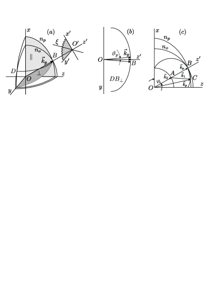
Figure 1: $(a)$ Octant of the refractive index surfaces $n_{e}({\vec{r}})$ and $n_{o}({\vec{r}})$ for pump and signal photons, $(b,c)$ are two perpendicular section by the planes $\perp$ and $\|$ shaded in $(a)$; $DB_{\perp}$ is the projection on the $\perp$-plane of the circle shown partially by the arc $DB$ in $(a)$; $\vartheta_{p}$ is the angle between ${\vec{k}}_{p}$ and the $z^{\prime}$ axis.

the $Ox$ axis, and the orthogonal axes $Oy$ and $Oz$ are chosen in such a way that the $(xz)$ plane contains the pump laser axis $Oz^{\prime}$. The arc $DB$ in Fig. 1$(a)$ is a part of the circle by which the sphere and ellipsoid cross each other. We assume that the laser axis is directed strictly to the point $B$ where the arc $DB$ crosses the $xz$ plane. This means that for pump and emitted photons propagating strictly along the $z^{\prime}$-axis the collinear degenerate phase matching condition is exactly satisfied, ${\vec{k}}_{p}={\vec{k}}_{1}+{\vec{k}}_{2}$ at ${\vec{k}}_{p}\,\|\,{\vec{k}}_{1}\,\|\,{\vec{k}}_{2}\,\|\,Oz^{\prime}$, $k_{1}=k_{2}=k_{p}/2$. In our consideration we assume that the pump is not a single plane wave but is given by a coherent superposition of plane waves with wave vectors ${\vec{k}}_{p}$ filling in a cone, the axis of which coincides with the $Oz^{\prime}$ axis, and the angular width $\alpha$ is finite.

$O^{\prime}$ in Fig. 1($a$) is some point in a far zone located at the laser axis $Oz^{\prime}$ and such that detectors registering photons are located in the plane perpendicular to $Oz^{\prime}$ and containing the point $O^{\prime}$. The axes $O^{\prime}x^{\prime}$ and $O^{\prime}y^{\prime}$ in this plane are perpendicular to each other and to $O^{\prime}z^{\prime}$, and $O^{\prime}x^{\prime}\in(xz)$, $O^{\prime}y^{\prime}\|Oy$. Let us assume that detectors are installed along some line $O^{\prime}\xi$ in the plane $(x^{\prime}y^{\prime})$ and, hence, they register only photons (1) and (2) with wave vectors ${\vec{k}}_{1}$ and ${\vec{k}}_{2}$ belonging to the plane ($z^{\prime}\xi$). Orientation of the detector-installation line $O^{\prime}\xi$ in the plane ($x^{\prime}y^{\prime}$) can be changed with two limiting cases given by $O^{\prime}\xi=O^{\prime}y^{\prime}\|Oy$ and $O^{\prime}\xi=O^{\prime}x^{\prime}\in(xz)$ . In these two limiting cases the detectors register only photons with wave vector ${\vec{k}}_{1}$ and ${\vec{k}}_{2}$ belonging, correspondingly, to the $yOz^{\prime}$ and $xOz$ planes. In Fig. 1$(a)$ these planes are shaded and they are labeled with the symbols $\perp$ and $\|$, respectively. Here “perpendicular$"$ and “parallel$"$ mean that the observation plane (i.e., the plane containing wave vectors of photons to be observed) is perpendicular or parallel to the plane containing the crystal optical axis and the laser axis. Below these two cases are referred to as those of the perpendicular and parallel geometry. Sections of the $3D$ refractive index surfaces by the $\perp$ and $\|$ planes are shown in the pictures $(b)$ and $(c)$ of Fig. 1.

Note that the idea of changing orientation of the detector-installation line is used here for simplification of illustrations like those given in Fig. 1. In real experiment the laser pump axis was horizontal ($\|\,Oz$), and detectors were installed in such a way that they registered only photons with horizontally oriented wave vectors ${\vec{k}}_{1}$ and ${\vec{k}}_{2}$. This was a crystal that was rotated around the laser axis (together with the laser polarization) instead of changing detector positions. There are the following rules of one-to-one correspondence between these experimental conditions and the above-described geometries of Fig. 1: (1) orientation of the crystal optical axis in the horizontal plane $(yz)$ is equivalent to the $\|$ geometry and (2) orientation of the crystal optical axis in the vertical plane $(xz)$ is equivalent to the $\perp$ geometry of Fig. 1.

The second note concerns an additional assumption to be used below for simplicity and not motivated by orientation reasons. In terms of notations used in Fig. 1$(a)$, let us assume that the photons (1) and (2) with wave vectors ${\vec{k}}_{1}$ and ${\vec{k}}_{2}$ belonging to the plane $(z^{\prime}\xi)$ arise only owing to the decay of pump photons with wave vectors ${\vec{k}}_{p}$ belonging to the same plane $(z^{\prime}\xi)$. Rigorously, this is not necessarily true: owing to the non-collinear phase matching processes photons (1) or (2) can be emitted with wave vectors ${\vec{k}}_{1}$ or ${\vec{k}}_{2}$ belonging to the plane $(z^{\prime}\xi)$ even if the pump wave vector ${\vec{k}}_{p}$ is oriented differently. Such processes can affect the single-particle momentum distributions of emitted photons, and this effect is discussed below. But, on the other hand, the non-collinear phase matching processes can be effectively suppressed by means of axially asymmetric focusing of a laser beam. This possibility is also discussed below and its experimental realization is presented.

Under the formulated assumptions, with the help of the results derived by Monken et al in 1998 Monken1 , in the approximation of a wide crystal we can write down immediately the following expression for the biphoton wave function depending on the transverse components of the emitted photon momenta ${\vec{k}}_{1\,\xi}$ and ${\vec{k}}_{2\,\xi}$

$$\Psi(k_{1\,\xi},\,k_{2\,\xi})\propto E_{p}^{*}(k_{1\,\xi}+k_{2\,\xi})\times\mathrm{sinc}\left(\frac{L\,\Delta_{z^{\prime}}}{2}\right),$$ (2)

where ${\rm sinc}(u)=\sin(u)/u$, $L$ is the crystal length in the $z^{\prime}$-direction, and $\Delta_{z^{\prime}}$ is the longitudinal detuning

$$\Delta_{z^{\prime}}=k_{p\;z^{\prime}}-k_{1\,z^{\prime}}-k_{2\,z^{\prime}}\quad\quad\quad$$

$$=\sqrt{k_{p}^{2}-k_{p\,\xi}^{2}}-\sqrt{k_{1}^{2}-k_{1\,\xi}^{2}}-\sqrt{k_{2}^{2}-k_{2\,\xi}^{2}}.$$ (3)

The above-mentioned approximation of a wide crystal means that its size in the direction parallel to the $O^{\prime}\xi$ axis is large enough to make the transverse momentum conservation rule, or transverse phase matching condition, exactly satisfied to give $k_{p\,\xi}=k_{1\,\xi}+k_{2\,\xi}$. This relation is used in the definition of the momentum-dependent pump field-strength amplitude in Eq. (2), $E_{p}^{*}(k_{p\,\xi})=E_{p}^{*}(k_{1\,\xi}+k_{2\,\xi})$, and it can be used also in the definition of the longitudinal detuning $\Delta_{z^{\prime}}$ (3).

To simplify further Eq. (3) for the longitudinal detuning we can use the near-axis approximation in which $|k_{1,2\,\xi}|\ll k_{1,2}$, $k_{p\,\xi}\ll k_{p}$. By expanding square roots in Eq. (3) in powers of transverse components of all the wave vectors and keeping only two first orders we get

$$\Delta_{z^{\prime}}=k_{p}-k_{1}-k_{2}+\frac{(k_{1\,\xi}-k_{2\,\xi})^{2}}{2k_{p}}\,,$$ (4)

where in the second term on the right-hand side we took $k_{p}\approx 2k_{1}=2k_{2}$. As for the first term, $k_{p}-k_{1}-k_{2}$, if it can be taken equal zero identically, then Eqs. (2) and (4) give immediately the well-known and widely used formula of the work Monken2

$$\Psi(k_{1\,\xi},\,k_{2\,\xi})\propto E_{p}^{*}(k_{1\,\xi}+k_{2\,\xi})\mathrm{sinc}\left(\frac{L\,(k_{1\,\xi}-k_{2\,\xi})^{2}}{4k_{p}}\right).$$ (5)

This is the formula that is most often met and used for theoretical description of the SPDC biphoton entanglement. Eq. (5) has a form very close to that of the double-Gaussian wave function given by Eq. (1). Indeed, very often the pump envelope has a Gaussian form. As for the sinc²-function, it can be rather successfully modeled by a Gaussian function too Eberly-Law . The key point of such a reduction to the double Gaussian form is the separation of variables $k_{1\,\xi}$ and $k_{2\,\xi}$ for their two independent linear combinations $k_{1\,\xi}+k_{2\,\xi}$ and $k_{1\,\xi}-k_{2\,\xi}$ in the arguments of two protofunctions of Eq. (5), $E_{p}^{*}$ and sinc. As we will show now, such separation of variables and reduction of the wave function to the double-Gaussian form essentially depend on the assumption $k_{p}-k_{1}-k_{2}\equiv 0$ which is true only under very special conditions.

As it can be seen from the pictures of Fig. 1, the collinear phase matching condition $k_{p}-k_{1}-k_{2}=0$ can be taken satisfied for different orientations of the pump wave vector ${\vec{k}}_{p}$ only if the detection direction $O^{\prime}\xi$ is perpendicular to the plane containing the laser and crystal optical axes, i.e., if $O^{\prime}\xi\|Oy$. In this case, for all wave vectors ${\vec{k}}_{p}$ located in the $\perp$-plane of Fig. 1$(a)$ and not too far deviating from the $Oz^{\prime}$ axis, their length can be taken approximately equal: $k_{p}(\vartheta_{p})\approx k_{p}(0)=k_{1}+k_{2}$, where $\vartheta_{p}$ is the angle between ${\vec{k}}_{p}$ and $Oz^{\prime}$, $|\vartheta|\ll 1$. Owing to the last condition the arc $DB_{\perp}$ in Fig. 1$(b)$ can be approximated by an arc of a circle with the center at the origin $O$, and then equality of all wave vector lengths $k_{p}(\vartheta)$ becomes evident.

At all other orientations of the detector-installation line $O^{\prime}\xi$, non-parallel to $Oy$ direction, the difference $k_{p}(\vartheta_{p})-k_{1}-k_{2}$ on the right-hand side of Eq. (4) cannot be taken equal zero at $\vartheta_{p}\neq 0$ even approximately. At small values of $\vartheta_{p}$ the dependence $k_{p}(\vartheta_{p})$ can be linearized to give

$$k_{p}(\vartheta_{p})=\frac{\omega}{c}\,n_{p}(\varphi_{0}+\vartheta_{p})\approx k_{p}(0)\left[1+\vartheta_{p}\frac{n_{p}^{\prime}(\varphi)}{n_{p}(\varphi)}\right]_{\varphi=\varphi_{0}}\,,$$ (6)

where $n_{p}^{\prime}(\varphi)=dn_{p}(\varphi)/d\varphi$, $\varphi$ is the angle between ${\vec{k}}_{p}$ and the crystal optical axis ($Ox$ in Fig. 1) and $\varphi_{0}$ is the angle between the optical and laser axes. On the other hand, as the laser axis $Oz^{\prime}$ and the detector-installation line $O^{\prime}\xi$ are perpendicular to each other, at small $\vartheta_{p}$ we have $k_{p}(0)\,\vartheta_{p}\approx k_{p\,\xi}=k_{1\,\xi}+k_{2\,\xi}$. By remembering that $k_{p}(\vartheta_{p}=0)=k_{1}+k_{2}$ and combining all these relations together we get the following expression for the longitudinal detuning $\Delta_{z^{\prime}}$

$$\Delta_{z^{\prime}}=\frac{n_{p}^{\prime}}{n_{o}}(k_{1\,\xi}+k_{2\,\xi})+\frac{(k_{1\,\xi}-k_{2\,\xi})^{2}}{2k_{p}}$$ (7)

and for the momentum biphoton wave function

$$\Psi(k_{1\,\xi},\,k_{2\,xi})\propto E_{p}^{*}(k_{1\,\xi}+k_{2\,\xi})\quad\quad\quad$$

$$\times\,\mathrm{sinc}\left\{\ \frac{L}{2}\left[\frac{n_{p}^{\prime}}{n_{o}}(k_{1\,\xi}+k_{2\,\xi})+\frac{(k_{1\,\xi}-k_{2\,\xi})^{2}}{2k_{p}}\right]\right\}\,,$$ (8)

where $n_{p}^{\prime}=n_{p}^{\prime}(\varphi_{0})$ and $n_{o}=n_{p}(\varphi_{0})$. Eq. (8) is the main new formula for the biphoton wave function we suggest instead of the traditional one given by Eq. (5). These two formulas differ from each other by the first term in the sum in square brackets under the symbol of the ${\rm sinc}-$function in Eq. (8). Below we will analyze how important this addition is. But before doing this, let us rewrite Eq. (8) in terms of the scattering angles $\theta_{1}$ and $\theta_{2}$, defined outside the crystal as $\theta_{1,\,2}=2k_{1,\,2\;\xi}/k_{p}^{(0)}$, where $k_{p}^{(0)}=\omega_{p}/c$. By using these definitions we express the transverse components of the emitted photon wave vectors via the scattering angles and reduce Eq. (8) to the form

$$\Psi(\theta_{1},\,\theta_{2})\propto{\widetilde{E}}_{p}^{*}\left(\frac{\theta_{1}+\theta_{2}}{2}\right)\quad\quad\quad$$

$$\times\,{\rm sinc}\left\{\displaystyle\frac{Lk_{p}^{(0)}}{16n_{o}}\Big{[}4n_{p}^{\prime}(\theta_{1}+\theta_{2})+(\theta_{1}-\theta_{2})^{2}\Big{]}\right\}\,,$$ (9)

where ${\widetilde{E}}_{p}(\theta_{p})$ is the pump amplitude angular distribution outside the crystal, $\theta_{p}=\frac{1}{2}(\theta_{1}+\theta_{2})=n_{o}\vartheta_{p}$ (to remind, by definition $\vartheta_{p}$ is the angle between ${\vec{k}}_{p}$ and the laser axis $Oz^{\prime}$ in a crystal) . In terms of scattering angles the longitudinal detuning of Eq. (7) appears to be given by

$$\Delta_{z^{\prime}}=\frac{k_{p}^{(0)}}{8}\Big{[}4n_{p}^{\prime}(\theta_{1}+\theta_{2})+(\theta_{1}-\theta_{2})^{2}\Big{]}.$$ (10)

The new first term in the square brackets of Eqs. (9) and (10) is linear whereas the second term is quadratic in small angles $\theta_{1}$ and $\theta_{2}$. For this reason we can expect that the linear term is even more important than the quadratic one, if only the refractive index derivative $n_{p}^{\prime}$ is not negligibly small. But this does not mean that the quadratic term can be dropped because in such an approximation we would get infinitely wide single-particle distributions. So, both linear and quadratic terms have to be taken into account. The role of the linear term is illustrated by three curves of Fig. 2 where

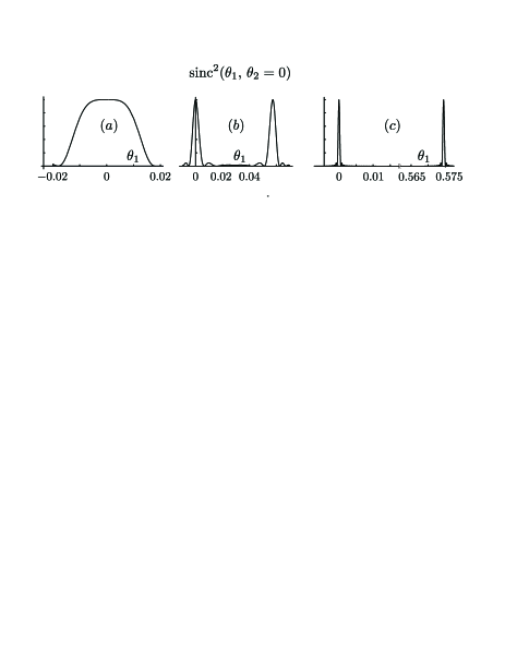
Figure 2: The function ${\rm sinc}^{2}(L\Delta_{z^{\prime}}/2)$ at $\theta_{2}=0$ and $(a)\,n_{p}^{\prime}=\,0,\,(b)\,-0.01436,\,\mathrm{and}\,(c)-0.1436$; $\theta_{1}$ is in radians.

the function ${\rm sinc}^{2}(L\Delta_{z^{\prime}}/2)$ is plotted in its dependence on $\theta_{1}$ at $\theta_{2}=0$ and at three different values of the refractive index derivative. The curves of Fig. 2 are calculated for the pump and crystal parameters corresponding to the experimental ones (see the following Section): the pump wavelength $\lambda_{p}=325$ nm and LiIO₃ crystal of a length $L=1.5\,{\rm}$ cm. In this case we have found $\varphi_{0}\approx 60^{\rm o}$ and $n_{p}^{\prime}=-0.1436$ for the detection of photons in the vertical plane of Fig. 1. The three curves of Fig. 2 correspond to $(a)\,n_{p}^{\prime}=0$ - photon propagation and detection in the horizontal plane, $(b)\,n_{p}^{\prime}=-0.01436$ - some intermediate case between $\perp$- and $\|$-geometries of Fig. 1$(a)$, and $(c)\,n_{p}^{\prime}=-0.1436$ - propagation and detection in the $\|$-plane. One can see, that with a growing value of $|n_{p}^{\prime}|$ the structure of the curves in Fig. 2 changes drastically. A single wide peak splits for two peaks, spacing between them grows, and the peaks themselves are getting very narrow. The widths of the only peak at $n_{p}^{\prime}=0$ and of narrow peaks at $n_{p}^{\prime}=-0.1436$ are equal to 24 mrad and 0.5 mrad, correspondingly. The ratio of these two widths equals to 48 and this number characterizes the degree of peak narrowing arising owing to modifications in the formula of Eqs. (8), (9) compared to that of Eq. (5).

Mathematically splitting of a single peak for two ones follows from the quadratic dependence of the detuning $\Delta_{z^{\prime}}$ (10) on $\theta_{1}$. The ${\rm sinc}-$function is maximal at zero value of its argument, i.e., at zero detuning $\Delta_{z^{\prime}}$. In a general case the quadratic equation $\Delta_{z^{\prime}}(\theta_{1})=0$ has two solutions which correspond to two peaks in the dependence of sinc² on $\theta_{1}$. The only exception is the degenerate case $n_{p}^{\prime}=0$ when two solutions of the quadratic equation merge into one. Qualitatively the same conclusions and the same arguments are illustrated by the Fig. 1$(c)$. In this picture the vector ${\vec{k}}_{2}$ is plotted along the optical axis $Oz^{\prime}$ ($\theta_{2}=0$), and it ends at the point $A$. The ending locus for vectors ${\vec{k}}_{1}$ is given in this case by a circle of the radius $n_{0}/2$ (in units of $\omega_{p}/c)$ and with the center at the point $A$. As it’s seen from the picture, there are two points $B$ an $C$ where this circle crosses the ellipse $n_{p}(\theta_{p})$ which, in its turn, is the ending locus for the pump wave vectors ${\vec{k}}_{p}$. This picture shows that in the case $n_{p}^{\prime}\neq 0$ there are two directions of the vectors ${\vec{k}}_{1}$ and ${\vec{k}}_{p}$ (at a given ${\vec{k}}_{2}$) in which the exact phase matching condition ${\vec{k}}_{p}={\vec{k}}_{1}+{\vec{k}}_{2}$ appears to be fulfilled. Quantitatively, the nonzero angle of the second exact phase matching direction appears to be very large. The value of $\theta_{1}\approx 0.57$ in Fig. 2$(c)$ corresponds to about 30^o for the scattering angle $\theta_{1}$ and to $\theta_{p}\approx\,15^{\rm o}$ for the pump. As the last value is much larger than the pump angular divergence (typically $\alpha\sim 4\,{\rm mrad}\approx 0.23^{\rm o}$), the second (nonzero-angle) peak of the sinc² function does not give contributions to the single-particle photon momentum distributions (see the derivation and discussion below). The large-angle second peak of the sinc²-function was not observed also in the coincidence measurements described in the following Section simply because this was out of the detector scanning range. For these reasons we restrict our further analysis by considering only one peak of the sinc²-function located at small values of the scattering angle $\theta_{1}$ in both cases of zero and nonzero values of the refractive index derivative $n_{p}^{\prime}$.

The quadratic dependence of $\Delta_{z^{\prime}}$ on $\theta_{1}$ and a transition from the case when the equation $\Delta_{z^{\prime}}=0$ has a single solution to the case of two different solutions (at $n_{p}^{\prime}\neq 0$) explain also qualitatively the reasons of peak narrowing. Roughly the sinc² peak widths can be evaluated from the condition $|\Delta_{z^{\prime}}|\sim 1/L$. In the case $n_{p}^{\prime}=0$ at $\theta_{2}=0$ we have $\Delta_{z^{\prime}}\sim k_{p}^{(0)}\theta_{1}^{2}$ which gives $\Delta\theta_{1}\sim 1/\sqrt{Lk_{p}^{(0)}}$. In contrast, in the case $n_{p}^{\prime}\neq 0$ in a vicinity of each narrow peak the detuning is approximately linear in $\theta_{1}$, and from the same condition $|\Delta_{z^{\prime}}|\sim 1/L$ we find $\Delta\theta_{1}\sim 1/(Lk_{p}^{(0)})$. As the product $Lk_{p}^{(0)}$ is rather large ($\sim 10^{5}$), both width are small but the peak widths occurring in the case $n_{p}^{\prime}\neq 0$ is much smaller than that occurring in the case $n_{p}^{\prime}=0$, $1/(Lk_{p}^{(0)})\ll 1/\sqrt{Lk_{p}^{(0)}}$ .

II.2 Coincidence and single-particle distributions

Coincidence distributions of photons are given simply by the squared absolute value of the wave function $\Psi(\theta_{1},\,\theta_{2})$ of Eq. (9) at a given value of one of the angles, $\theta_{1}$ or $\theta_{2}$. E.g., at $\theta_{2}=0$

$$\frac{dw^{(c)}(\theta_{1})}{d\theta_{1}}\propto\left|\Psi\left(\theta_{1},\,0\right)\right|^{2}\quad\quad\quad$$

$$\propto\left|{\widetilde{E}}_{p}\left(\frac{\theta_{1}}{2}\right)\,{\rm sinc}\left[\frac{Lk_{p}}{16}\,\left(4n_{p}^{\prime}\,\theta_{1}+\theta_{1}^{2}\right)\right]\right|^{2}.$$ (11)

Single-particle distributions are given by the squared wave function of Eq. (9) integrated over, e.g., $\theta_{2}$. In the case $n_{p}^{\prime}\neq 0$ it is convenient to make the integration variable substitution $\theta_{2}\rightarrow\theta\equiv\theta_{2}+\theta_{1}$ (at a given value of $\theta_{1}$) to get

$$\frac{dw^{(s)}(\theta_{1})}{d\theta_{1}}\propto\int d\theta\left|{\widetilde{E}}_{p}\left(\frac{\theta}{2}\right)\,{\rm sinc}\left[\frac{L}{2}\,\Delta_{z^{\prime}}(\theta;\,\theta_{1})\right]\right|^{2},$$ (12)

where now

$$\Delta_{z^{\prime}}=\frac{k_{p}^{(0)}}{8}\Big{[}4n_{p}^{\prime}\theta+(\theta-2\theta_{1})^{2}\Big{]}.$$ (13)

At $n_{p}^{\prime}\neq 0$ the sinc²-function is not negligibly small only in small vicinity of points where the detuning $\Delta_{z^{\prime}}(\theta;\,\theta_{1})$ turns zero. From the condition $\Delta_{z^{\prime}}=0$ we get a quadratic equation in $\theta$, solutions of which are given by

$$\theta_{a,\,b}(\theta_{1})=2\left[\,\theta_{1}-n_{p}^{\prime}\mp\sqrt{n_{p}^{\prime\;2}-2n_{p}^{\prime}\theta_{1}}\;\right].$$ (14)

Only one of these two solutions ($\theta_{a}$) is small enough for a region around this point to give a non-zero contribution to the integral over $\theta$ in Eq. (12). Near the point $\theta_{a}$ the detuning $\Delta_{z^{\prime}}$ can be approximated by a linear function of $\theta$

$$\Delta_{z^{\prime}}\approx\frac{k_{p}^{(0)}}{2}\sqrt{n_{p}^{\prime\;2}-2n_{p}^{\prime}\theta_{1}}\;(\theta-\theta_{a})$$ (15)

and the sinc² function can be approximated by the delta function

$${\rm sinc}^{2}\left[\frac{L}{2}\Delta_{z^{\prime}}\right]\propto\frac{\delta(\theta-\theta_{a})}{\sqrt{n_{p}^{\prime\;2}-2n_{p}^{\prime}\theta_{1}}}$$ (16)

to give finally the following simple expression for the single-particle momentum distribution of photons

$$\frac{dw^{(s)}_{\|}(\theta_{1})}{d\theta_{1}}\propto\frac{\left|E_{p}\left[\displaystyle\frac{\theta_{a}(\theta_{1})}{2}\right]\right|^{2}}{\sqrt{n_{p}^{\prime\;2}-2n_{p}^{\prime}\theta_{1}}}$$ (17)

with $\theta_{a}(\theta_{1})$ given by Eq. (14).

The coincidence (solid lines) and single-particle (dashed lines) photon momentum probability distributions are plotted in Fig. 3 for two cases, $(a)\;n_{p}^{\prime}=0$ ($\perp$-geometry) and $(b)\;n_{p}^{\prime}\neq 0$ ($\|$-geometry). In both cases the dotted-line curves describe the pump intensity $|{\widetilde{E}}_{p}(\theta_{p})|^{2}$

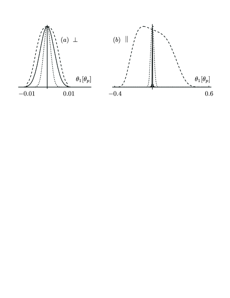
Figure 3: Coincidence (solid lines) and single-particle (dashed lines) photon distributions, $dw^{(c)}/d\theta_{1}$ (at $\theta_{2}=0$) and $dw^{(s)}/d\theta_{1}$, calculated for the cases $(a)$ $n_{p}^{\prime}=0$ and $n_{p}^{\prime}=-1.436$. The dotted-line curves show the pump intensity in its dependence on $\theta_{p}$. All curves are normalized by one at their maxima.

taken in the Gaussian form

$$|{\widetilde{E}}_{p}(\theta_{p})|^{2}\propto\exp\left[-\frac{4\ln{(2)}\,\theta_{p}^{2}}{\alpha^{2}}\right]$$ (18)

with $\alpha=0.004114$.

In the case $n_{p}^{\prime}=0$ ($\perp$-geometry) integration in Eq. (12) is performed numerically, whereas in the case $n_{p}^{\prime}\neq 0$ ($\|$-geometry) we used the analytical expression of Eq. (17). On the other hand, as in the case $n_{p}^{\prime}=0$ the sinc-function (Fig. 3$(a)$) is wider than the pump, the coincidence curve in the $\perp$-geometry is close to the pump angular distribution curve in its dependence on $(\theta_{1}+\theta_{2})/2$ at a given $\theta_{2}$. In particular, at $\theta_{2}=0$ the coincidence momentum probability distribution in the $\|$-geometry is given by

$$\frac{dw^{(c)}_{\perp}}{d\theta_{1}}\approx\left|E_{p}\left(\frac{\theta_{1}}{2}\right)\right|^{2}.$$ (19)

Validity of this equation is pretty well confirmed by the calculated coincidence and pump ($|{\widetilde{E}}_{p}(\theta_{p})|^{2}$) curves in Fig. 3$(a)$: the solid-line curve is twice wider than the dotted-line one.

As a whole, for the taken laser and crystal parameters, the case $n_{p}^{\prime}=0$ ($\perp$-geometry) does not provide conditions for observing high entanglement of the arising biphoton state. Indeed, the coincidence and single-particle distributions are seen in Fig. 3$(a)$ to be rather close to each other. Their widths are equal to $\Delta\theta_{1\,\perp}^{(c)}\approx 8$ mrad and $\Delta\theta_{1\,\perp}^{(s)}\approx 12$ mrad, which corresponds to the width ratio $R_{k\,\perp}=\Delta\theta_{1\,\perp}^{(s)}/\Delta\theta_{1\,\perp}^{(c)}\approx 1.5$. In reality the width $\Delta\theta_{1}^{(s)}$ and the ratio $R_{k\,\perp}$ can be slightly higher than estimated here because of the non-collinear phase matching processes to be discussed below. But this increase is not too high, and the main conclusion remains valid: the $\perp$-geometry does not provide conditions for observing high entanglement that can be accumulated in the biphoton state under consideration.

This high entanglement can be seen most successfully in the $\|$-geometry. The corresponding coincidence and single-particle momentum distributions are shown for this case in Fig. 3$(b)$. As in the $\|$-geometry ($n_{p}^{\prime}\neq 0$) the sinc-function in Eq. (11) is much narrower than the pump, the coincidence angular distribution is identical in this case to the narrow peak of the sinc²-function located near $\theta_{1}=0$ and described in Fig. 2$(c)$:

$$\frac{dw^{(c)}_{\|}(\theta_{1})}{d\theta_{1}}={\rm sinc}^{2}\left[\frac{Lk_{p}}{16}\,\left(4n_{p}^{\prime}\,\theta_{1}+\theta_{1}^{2}\right)\right].$$ (20)

The width of this peak found above gives us the coincidence width of the byphoton angular distribution in the $\|$-geometry: $\Delta\theta_{1\,\|}^{(c)}=0.5$ mrad. The single-particle angular distribution in the $\|$-geometry is determined by Eq. (17) and is shown in Fig. 3$(b)$ in the dashed-line curve. The width of this curve is equal to $\Delta\theta_{1\,\|}^{(s)}=47.3$ mrad. The ratio of these widths is the entanglement-parameter for measurements in the $\|$-geometry

$$R_{k\,\|}=\frac{\Delta\theta_{1\,\|}^{(s)}}{\Delta\theta_{1\,\|}^{(c)}}=\frac{47.3}{0.5}=94.6\gg 1\,.$$ (21)

In contrast to the earlier considered case of the $\perp$-geometry, the $\|$-geometry of measurements does provide conditions for observing very high degree of entanglement accumulated in the same biphoton state and not seen so well in other geometries of measurements.

Related to the estimate of the entanglement parameter $R_{k\,\|}$ (21), the two new specific effects predicted for the $\|$-geometry and differing it from the traditionally considered $\perp$-geometry are: (1) a very strong narrowing of the coincidence and (2) broadening of the single-particle distribution curves. The narrowing effect is very strong indeed: the width $\Delta\theta_{1\,\|}^{(c)}$ is 16 times smaller than the same width $\Delta\theta_{1\,\perp}^{(c)}$ occurring in the perpendicular geometry, and 8 times smaller than the pump angular width $\alpha$. This shows, in particular, that the coincidence angular distribution appears to be narrower than that of the pump (contrary to traditional expectations based on consideration of the $\perp$-geometry scheme). Explanation of this effect is related to drastic changes in the structure of the sinc-function in Eqs. (9) and (11) (see Fig. 2), which occur when we move from the $\perp$- to $\|$-geometry.

As for broadening of the single particle angular biphoton distribution in the $\|$-geometry, it has a rather simple qualitative explanation in terms of the non-collinear phase matching down-conversion processes. Their origin is illustrated by two pictures of Fig. 4. The first picture $[4(a)]$ is the same projection of the refractive index

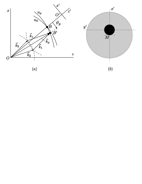
Figure 4: (a) Diagram of pump and emitted photon wave vectors under the conditions of non-collinear phase matching; dashed lines are arcs of circles with radii $n_{o}/2$ and centers at the points $O$ and $B^{\prime}$, wave vectors are in units of $\omega_{p}/c$. (b) Angular distributions of photons emitted in the regime of non-collinear phase matching (grey) and of the pump (black), a view along the $-Oz^{\prime}$ direction, $M$ is the point of the maximal achievable non-collinear phase matching.

surfaces as in Fig. 1$(c)$. But now the pump wave vector ${\vec{k}}_{p}$ is taken slightly deflected from the laser axis direction $Oz^{\prime}$ (upon the angle $\vartheta_{p}$). As ${\vec{k}}_{p}(\vartheta_{p})$ is shorter than ${\vec{k}}_{p}(0)$, its ending point $B^{\prime}$ cannot be reached by two collinear wave vectors ${\vec{k}}_{1}$ and ${\vec{k}}_{2}$, and these vectors must be non-collinear both to each other and to ${\vec{k}}_{p}(\vartheta_{p})$. As it’s seen from Fig. 4$(a)$, the wave vectors ${\vec{k}}_{1}$ and ${\vec{k}}_{2}$ providing fulfilment of the exact phase matching condition are emitted under angles (with respect to the $Oz^{\prime}$ axis) exceeding $\vartheta_{p}\,$. This explains why the non-collinear phase matching emission broadens the single-particle probability density curves.

By rotating the wave-vector diagram of Fig. 4$(a)$ around the direction of the pump wave vector ${\vec{k}}_{p}$ we get cones along which the non-collinear-emitted photons can propagate. The cone opening angle changes with changing $\vartheta_{p}$ by forming in such a way the total emission area. Schematically this area of emission (in the angular space) is shown in Fig. 4$(b)$ (shaded in grey). This area is seen to be wider than that of the pump (shaded in black) and it’s seen to be wide both in the $O^{\prime}x^{\prime}$ and $O^{\prime}y^{\prime}$ directions. The last case corresponds to detection of photons in the $\perp$-plane. Hence, as said above, emission of photons in the non-collinear phase matching regime can make the single-particle probability density distribution somewhat wider than that described by the dashed-line curve in Fig. 3$(a)$.

The point $M$ in Fig. 4$(b)$ indicates the maximal achievable angle $\vartheta_{p}$ evaluated, e.g., at a half-width of the pump angular distribution, $\vartheta_{p}=\alpha/2$. This value of $\vartheta_{p}$ provides the maximal emission cone opening angle, which is characterized by the circle in Fig. 4$(b)$ bordering the grey area and having its center at $M$. It’s seen in Fig. 4$(b)$ that the emission are area is asymmetric with respect to the point $O^{\prime}$ ($x^{\prime}$ and $z^{\prime}$ line crossing) in the $O^{\prime}x^{\prime}$ direction. This agrees with the structure of the single-particle probability density distribution in the case of detection in the $\|$-plane [the dashed-line curve of Fig. 3$(b)$]. The reason of asymmetry is evident: deflection of the pump wave vector ${\vec{k}}_{p}$ from the $Oz^{\prime}$ axis to the direction opposite to that shown in Fig. 4$(a)$ makes ${\vec{k}}_{p}$ longer than ${\vec{k}}_{p}(0)$. For such wave vectors, in contrast to the case considered above, the exact phase matching condition cannot be fulfilled at all and, hence, such deflections give almost zero contribution to the integral in Eq. (17) determining the single-particle probability density distribution.

Note that the role of photon emission in the regime of the non-collinear phase matching can be diminished by special profiling the pump angular distribution. In terms of Fig. 1 geometries, if the pump angular distribution is made narrow in the $O^{\prime}x^{\prime}$ direction but, still, remains wide enough in the $O^{\prime}y^{\prime}$ direction, then the point $M$ in Fig. 4$(b)$ approaches $O^{\prime}$ and the radius of the grey area decreases, thus making single-particle angular distributions narrower. In the extreme limit of the pump angular distribution very narrow in the $O^{\prime}x^{\prime}$ direction, in the case of photon detection in the $\perp$-geometry we return to the results described by the curves of Fig. 3$(a)$. Such an asymmetric profiling of the pump angular distribution can be provided by focusing with a cylindrical lens or by a slit.

So, the used above simplification that the essential pump wave vectors ${\vec{k}}_{p}$ belong to the same plane as ${\vec{k}}_{1}$ and ${\vec{k}}_{2}$ can be not too good for describing the single-particle angular photon distribution in the $\perp$-geometry. But this simplification does not affect both coincidence distributions at arbitrary orientation of the observation plane $(z^{\prime}\xi)$ and any distributions in the $\|$-geometry.

II.3 Coordinate representation

The biphoton wave function in the coordinate representation can be obtained from the momentum-representation wave function by means of a double Fourier transformation

$$\Psi_{\rm coord}(\xi_{1},\,\xi_{2})=\int dk_{1\,\xi}\,dk_{2\,\xi}\,\Psi_{\rm mom}(k_{1\,\xi},\,k_{2\,\xi})$$

$$\times\exp\big{[}i(\xi_{1}k_{1\,\xi}+\xi_{2}k_{2\,\xi})\big{]},\quad\quad\quad$$ (22)

where $\xi_{1}$ and $\xi_{2}$ are coordinates along the observation direction $O^{\prime}\xi$ for photons (1) and (2) and $\Psi_{\rm mom}(k_{1\,\xi},\,k_{2\,\xi})$ is the same function as $\Psi(k_{1\,\xi},\,k_{2\,\xi})$ of Eq. (8). Integrations in Eq. (22) can be carried out partially in a rather simple way only in the case of a sufficiently large refractive index derivative. So let us consider only the $\|$-geometry when the detection direction $O^{\prime}\xi$ coincides with $O^{\prime}x^{\prime}$. The integration variables $k_{1\,x^{\prime}}$ and $k_{2\,x^{\prime}}$ can be substituted by the angular variables $\theta_{p}=(k_{1\,x^{\prime}}+k_{2\,x^{\prime}})/k_{p}^{(0)}$ and $\theta=(k_{1\,x^{\prime}}-k_{2\,x^{\prime}})/k_{p}^{(0)}$. In these variables the sinc-function in (8) takes the form convenient for its subsequent approximation by the $\delta$-function:

$${\rm sinc}\left[\frac{Lk_{p}^{(0)}}{2n_{o}}\left(n_{p}^{\prime}\theta_{p}+\frac{\theta^{2}}{2}\right)\right]\propto\delta\left(\theta_{p}+\frac{\theta^{2}}{2n_{p}^{\prime}}\right)\,.$$ (23)

In this approximation and with the pump amplitude ${\widetilde{E}}_{p}$ taken in the Gaussian form [Eq. (18)], Eq. (22) yields

$$\Psi_{\rm coord}(x^{\prime}_{1},\,x^{\prime}_{2})\propto\int d\theta\exp\left\{-\frac{\ln(2)\theta^{4}}{2\alpha^{2}n_{p}^{\prime\;2}}\right.$$

$$+i\,k_{p}^{(0)}\left.\left[-\frac{x^{\prime}_{1}+x^{\prime}_{2}}{4n_{p}^{\prime}}\,\theta^{2}+\frac{x^{\prime}_{1}-x^{\prime}_{2}}{2}\,\theta\right]\right\}\,.$$ (24)

The $\delta$-function approximation of (23) and the final expression of Eq. (24) are valid the sinc-function on the left-hand side of Eq. (23) is narrower than the pump ${\widetilde{E}}_{p}(\theta_{p})$ of Eq. (18), which gives

$$\frac{Lk_{p}^{(0)}|n_{p}^{\prime}|}{2n_{0}}\gg\frac{2}{\alpha}\,.$$ (25)

With $L$, $\alpha$, and $k_{p}^{(0)}$ we use in this paper the left- and right-hand sides of this inequality are equal to $1.1\times 10^{4}$ and 486, correspondingly, and the condition of Eq. (25) is pretty well satisfied. Under the condition (25) the coordinate biphoton wave function (24) does not depend on the crystal length $L$. Its features are fully controlled by the pump angular divergence $\alpha$.

The biphoton coincidence coordinate distribution $dw^{(c)}/dx_{1}^{\prime}|_{x_{2}^{\prime}=0}\propto|\Psi_{\rm coord}(x_{1}^{\prime},\,0)|^{2}$ calculated with the help of Eq. (24) is plotted in Fig. 5 in its dependence on

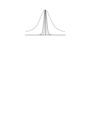
Figure 5: Coincidence probability density in the coordinate representation in its dependence on $x_{1}^{\prime}k_{p}^{(0)}/2$ (solid line); dependence of the bipartite probability density on $(x_{1}+x_{2})k_{p}^{(0)}/2$ at $x_{1}-x_{2}=0$ (dashed line) and on $(x_{1}-x_{2})k_{p}^{(0)}/2$ at $x_{1}+x_{2}=0$ (dotted line).

the dimensionless product $x_{1}^{\prime}k_{p}^{(0)}/2$ (the solid-line curve). In the same picture the probability density $|\Psi_{\rm coord}|^{2}(x_{1}^{\prime},x_{2}^{\prime})$ is plotted in its dependence on $\xi_{+}\equiv(x_{1}^{\prime}+x_{2}^{\prime})k_{p}^{(0)}/2$ at $\xi_{-}\equiv(x_{1}^{\prime}-x_{2}^{\prime})k_{p}^{(0)}/2=0$ (the dashed-line curve) and on $\xi_{-}$ at $\xi_{+}=0$ (the dotted-line curve). The widths of these curves are equal to $\Delta x_{1}^{\prime\,(c)}k_{p}^{(0)}/2=88$, $\Delta\xi_{+}=356.4$, and $\Delta\xi_{-}=44$. The distribution is seen to be much wider in the $\xi_{+}$ than in $\xi_{-}$ direction.

We did not calculate (yet) the single-particle probability density in the coordinate representation. But we can use the found width of the coincidence coordinate distribution for evaluating the EPR-related parameter of entanglement. Indeed, by taking into account that $\Delta k_{1\,x^{\prime}}=\Delta\theta_{1}\times k_{p}^{(0)}/2$, we get for the $\|$-geometry: $\Delta k_{1\,x^{\prime}}^{(c)}\times\Delta x_{1}^{\prime\,(c)}=0.0005\times 88=0.0044$ and $C_{\rm EPR}=1/\Delta k_{1\,x^{\prime}}^{(c)}\times\Delta x_{1}^{\prime\,(c)}=22.7$. By taking into account that in the no-entanglement case for Gaussian functions and for our definitions of widths as the half-height widths $C_{\rm EPR}^{(0)}=(4\ln 2)^{-1}$, we find finally the the EPR related parameter of entanglement for the $\|$-geometry is evaluated as

$$\frac{C_{\rm EPR}}{C_{\rm EPR}^{(0)}}=22.7\times 4\ln 2=63.$$ (26)

Though less than 80, this parameter is also rather large and indicates clearly that SPDC biphoton states under consideration are rather highly entangled.

III Experiment

III.1 Experimental setup

The experimental setup is shown on Fig.3. To generate the entangled photons we use type I and $15$ mm-length lithium-iodate crystal pumped with a 5 mW cw- helium-cadmium laser operating at $325$ nm. The correlated photons generated via SPDC process with equal polarization and wavelength $650$ nm are separated from the pump by dichroic mirror (DM). Interference filters centered at $650$ nm with a bandwidth of $10$ nm are placed in each arm of Brown-Twiss scheme. To measure coincidence and single-photon distributions in the transverse momenta we use the lens with focal length $F=62$ cm. Two single photon detectors are positioned in focal plane of the lens. Such detector arrangement allows one to measure the momentum distribution(s) by scanning one or both detectors along with certain direction (see below). In the most of cases we fix position of the first detector at the maximum of count rate and scan another one to register both distributions as a function of detector displacement. Since detector moves in the focal plane its position ($x$) relates to the angular mismatch $(\theta)$ as $x=F\tan\theta$.

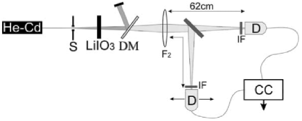
Figure 6: Experimental setup for measuring single and coincidence probability distributions.

III.2 Results and discussion

The main idea behind performed experiment is to check formulas (17), (20) and (19) for two geometries such that detectors are scanned (*) in the $\|$-plane containing optical axis, when $O^{\prime}\xi=O^{\prime}x^{\prime}\in(xz)$, and (**) in the $\perp$-plane, when $O^{\prime}\xi=O^{\prime}y^{\prime}\|Oy$ (see Fig. 1). One of the key parameters of the theory described above is the pump angular width. Originally our He-Cd laser had the angular width equal to 1.5 mrad. To see in experiment how the angular distrubution of the pump affects upon biphoton angular distributions, we have artificially and anisotropically broadened the pump distribution in angles by installing in front of the crystal a slit. As a result, the pump angular distribution remains localized along the direction parallel to the slit (at the same level of 1.5 mrad as was without a slit) but it spreads in the orthogonal direction. The slit was measured to be 40 mkm wide, which corresponds to the pump angular width in the direction perpendicular to the slit equal to 4.1 mrad. Alternatively we have used in some measurements a lens instead of a slit to provide axially symmetric (isotropic) broadening of the pump up to the same width of 4.1 mrad. Comaprison of results of such measurements was used for evaluating the role of the pump angular broadening for efficiency of emission processes arising under the non-collinear phase matching conditions.

As mentioned above, in the experiment the detection plane was always horizontal. The slit was installed always vertically to provide angular broadening in the horizontal direction, whereas the crystal optical axis could be lying either in the vertical or horizontal planes. In terms of notations and definitions used above and introduced in the picture of Fig. 1$(a)$ this means that our experimental measurements correspond to one of the following two situations: (A) detection and pump angular broadening directions are along the $O^{\prime}x^{\prime}$ axis, i.e., in the $\|$-plane or in the plane containing laser and optical axes and (B) both detection and pump angular broadening directions are along the $O^{\prime}y^{\prime}$ axis, i.e., in the $\perp$-plane, and these directions are perpendicular to the plane containing laser and optical axes. In the case when lens is used for the pump broadening it provides equal angular broadening in $O^{\prime}x^{\prime}$ and and $O^{\prime}y^{\prime}$, independently of the detection direction. As in the case $B$ the slit-broadened pump angular distribution is narrow in the $O^{\prime}x^{\prime}$ direction, we expect that under these conditions non-collinear phase matching processes will be suppressed [see the explanantion in Fig. 4$(b)$] and the single-particle angular distribution in the direction $O^{\prime}y^{\prime}$ will be narrower than in the case of lens angular broadening.

Another key parameter is angular derivative of the pump extraordinary refractive index $n_{p}^{\prime}$ near the exact phase matching direction $Oz^{\prime}$. The table 1 shows this value for different crystals available for producing photon pairs. It shows that Lithium Iodate is the best candidate because in this crystal the derivative $|n_{p}^{\prime}|$ takes a rather large value. Besides, the effect of high entanglement anisotropy discussed in the paper depends strongly on the product $Ln_{p}^{\prime}$. So, the second reason why we chose this crystal is that the sample of lithium iodate can be made rather long.

Crystal	phase matching angle $\varphi_{0}$ (deg.)	$n_{p}^{\prime}$
$LBO$	$51.47$	$-0.0270$
$KDP$	$54.33$	$-0.0395$
$BBO$	$36.44$	$-0.1175$
$LiIO_{3}$	$5.97$	$-0.1409$

Table 1: Angular anisotropy parameter $n_{p}^{\prime}$ for different non-linear crystals

As it follows from theory developed above, at sufficiently high values of $|n_{p}^{\prime}|$ the coincidence angular distribution of biphotons does not depend at all on the divergence of the pump [see Eq. (20)]. Moreover, being determined completely by properties of the crystal and, in particular, by anisotropy of the refractive index, the width of the coincidence distribution can be done even narrower than the pump angular width because. At the same time the width of the single-photon distributions grows up with the pump broadening. Both narrowing of the coincidence and broadening of the single-particle angular distributions are factors resulting in a growing degree of entanglement.

The pictures of Fig. 7 show two sets of angular distributions received in (a) single-particle and (b) coincidences measurements, which are plotted together for different geometries, with a slit broadened

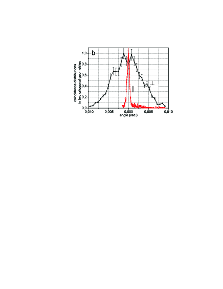
Figure 7: Angular distributions of (a) single and (b) coincidences counts for two orthogonal geometries ($\perp$) and ($\|$).

pump beam. These pictures illustrate clearly that in the $\|$-geometry coincidence distribution becomes narrower whereas the single-particle distribution broadens in comparison with the $\perp$-geometry. The corresponding ratios are $\Delta k_{\perp}^{(c)}/\Delta k_{\|}^{(c)}$=11 for coincidences and $\Delta k_{\perp}^{(s)}/\Delta k_{\|}^{(s)}$=0.41 for singles. For comparison, the corresponding theoretical estimates are $\Delta k_{\perp}^{(c)}/\Delta k_{\|}^{(c)}\approx 16$ and $\Delta k_{\perp}^{(s)}/\Delta k_{\|}^{(s)}\approx 0.25$. The difference between theoretical and experimental results is not too high, though quite visible. Probably, it has different origin for coincidence and single width ratios. In the case of coincidence counts, we think that the main reason for a difference between the theoretical and experimental width ratios is related to some external factors owing to which the experimentally measured coincidence width is larger than the theoretical estimate (0.75 mrad in experiment compared to 0.5 mrad in theory). As for the single-particle width, probably in experiment the corresponding curve in the $\perp$-geometry did experience some broadening arising from the non-collinear phase matching emission processes, in spite of the missing slit-broadening of the pump angular distribution in the $O^{\prime}x^{\prime}$ direction. In contrast to this, in theory presented above in the $\perp$-geometry case the non-collinear phase matching emission processes were completely excluded because only pump photons with wave vectors belonging to the observation plane were taken into account. Hence, compared to the real experimental situation, the given above theoretical derivation of the single-particle angular distribution in the $\perp$-geometry artificially narrows the corresponding curve, and this is the reason for the observed discrepancy between theory and experiment. But let us emphasize once again: the discrepancy is not too high, and the degree of closeness of theoretical and experimental results can be considered as quite satisfactory.

Figs. 8 and 9 present the same experimental results only differently regrouped, which allows one to evaluate the experimentally found degree of entanglement.

Fig. 8 corresponds to the case when detector is scanning in the plane perpendicular to the optical axis ($\perp$-geometry), and the slit broadens the pump angular distribution in the same direction. The width of the single-

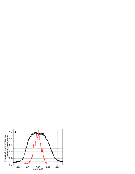
Figure 8: Experimental results: normalized single-particle and coincidence distributions for $\perp$-geometry. Curves with errors are the coincidence. The pump is broadened by a slit.

particle distribution is 25 mrad whereas the width of the coincidence one is 8.4 mrad, i.e., twice wider than the width of the pump [in accordance with Eq. (19)]. The ratio $\frac{\Delta k^{(s)}_{1\,\perp}}{\Delta k^{c}{(s)}_{1\,\perp}}=3$, so the degree of entanglement is not very high. Note, that in the above-presented theory we got for this ratio the twice smaller value, 1.5. The reason is the same as discussed above: in theory the single-particle angular distribution is artificially narrowed because all non-collinear phase matching processes are completely excluded from the consideration.

The results occurring in the case when both scanning and pump broadening occur in the plane containing the crystal optical axis ($\|$-geometry) are shown in Fig. 9. Here the widths of single- and coincidence distributions

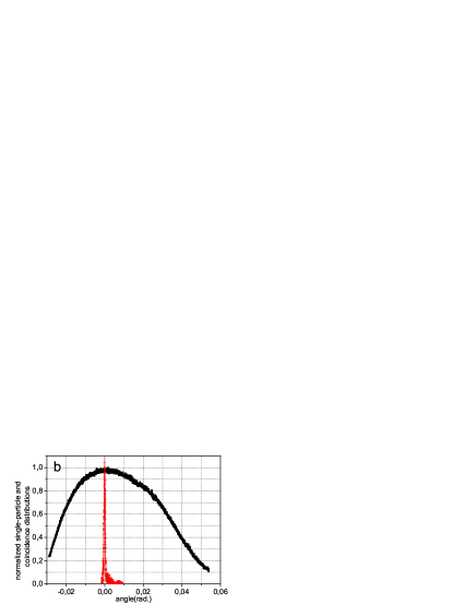
Figure 9: Experimental results: normalized single-particle and coincidence distributions for $\|$-geometry. Curves with errors are the coincidence. The pump is broadened by a slit.

are 60 mrad and 0.75 mrad correspondingly. Their ratio is 80, which is much greater than in previous case though is somewhat less than the corresponding theoretical estimate $R_{k\,\|}=94.6$ (21). The difference can be attributed only to some external factors affecting experiment. In the case of the $\|$-geometry the above-discussed non-collinear phase matching processes are completely taken into account in the theoretical derivation, and the explanation of the theory-experiment discrepancies given above for the $\perp$-geometry does not work for the $\|$-geometry.

Fig. 10 presents similar graphs but measured for the case when the laser pump is broadened with a spherical lens. This means that the pump broadening affects angular distributions in both directions and so, it is impossible to distinguish its contribution to spreading in $\|$- or $\perp$-planes. According to the picture of Fig.4$(b)$, the single-particle distribution measured in $\perp$-plane must be wider when the pump angular distribution is broadened by a lens compared to the case of broadening by a slit. This expectation is confirmed by measurements which give (for the $\perp$-geometry) $\Delta k_{(\rm lens)}^{(s)}/\Delta k_{(\rm slit)}^{(s)}$=0.075/0.025=3. However, another observed effect remains unexplained: for the same $\perp$-geometry the coincidence width in the case of lens-broadening appears to be smaller than in the case slit-broadening, $\Delta k_{(\rm lens)}^{(c)}/\Delta k_{(\rm slit)}^{(c)}$=0.0031/0.0084=0.37. Note also that in the case of lens broadening the values of the entanglement parameter $R_{k}$ appear to be somewhat smaller than in the case of slit broadening in both $\perp$- and $\|$-geometries: in the case of lens broadening $R_{k\,\perp}=2.33$ and $R_{k\,\|}=67$. But the main qualitative conclusions remain the same as earlier: at chosen values of the parameters almost no entanglement can be seen in the $\perp$-geometry and a very high entanglement can be and was observed in the $\|$-geometry.

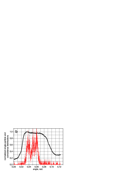
Figure 10: Experimental results: normalized single-particle and coincidence distributions for (a) $\|$- and (b) $\perp$-geometries. Curves with errors are the coincidence. The pump is broadened by a lens.

In conclusion, we have shown both theoretically and experimentally that there are two different schemes of observing SPDC biphoton wave packets. In the traditional and alternative schemes the detector scanning is assumed to be performed in the planes, correspondingly, perpendicular and parallel to the plane containing optical and laser axes. Owing to the anisotropy of the crystal refractive index for the extraordinary wave, a structure of the coincidence and single-particle biphoton wave packets observable in these two schemes are significantly different. In the alternative scheme, coincidence wave packets demonstrate a very strong narrowing compared to the traditional scheme, whereas the single-particle wave packets broaden. All this results in a very high degree of entanglement that can be observed in the alternative scheme of observations, and cannot be seen in the traditional scheme. The entanglement parameter determined as the ratio of the single to coincidence wave packet widths appears to be as high as about 100. The degree of the coincidence wave packet narrowing is shown to be so strong that in the alternative scheme of observations the coincidence wave packet appears to be much narrower than the angular distribution of the pump.

IV Acknowledgments

This work was supported in part by the Russian Foundation for Basic Research (projects 05-02-16469 and 06-02-16769), the RF President’s Grant MK1283.2005.2, the Leading Russian Scientific Schools (project 4586.2006.2), and by the US Army International Technology Center - Atlantic, grant RUE1-1616-MO-06.

References

- (1) A. Einstein, B. Podolsky, and N. Rosen, Phys. Rev. 47, 777 (1935).
- (2) E. Schrödinger, in Quantum Theory and Measurement, edited by J. A. Wheeler and W. H. Zurek Princeton University Press, New York, (1983).
- (3) M.H. Rubin, Phys. Rev. A 54, 5349 (1996)
- (4) A.V. Burlakov, M.V. Chekhova, D.N. Klyshko, S.P. Kulik, A.N. Penin, Y.H. Shih, and D.V. Strekalov, Phys. Rev. A 56, 3214 (1997).
- (5) C.H. Monken, P.H. Souto Ribeiro, and S. Padua, Phys. Rev. A 57, 3123 (1998).
- (6) S.P. Walborn, A.N. de Oliveira, and C.H. Monken, Phys. Rev. Lett. 90, 143601 (2003).
- (7) M.D’Angelo, Y.-H.Kim, S.Kulik, and Y.Shih, Phys. Rev. A 92, 233601 (2004).
- (8) C.K. Law and J.H. Eberly, Phys. Rev. Lett. 92, 127903 (2004).
- (9) J.C. Howell, R.S. Bennink, S.J. Bentley, and R.W. Boyd, Phys. Rev. Lett. 92, 210403 (2004).
- (10) M.V. Fedorov, M.A. Efremov, P.A. Volkov, and J.H. Eberly, J. Phys. B: At. Mol. Opt. Phys. 9, S467 (2006).
- (11) K.W. Chan, C.K. Law and J.H. Eberly, Phys. Rev. A. 68, 022110 (2003).
- (12) R. Grobe, K. Rzazewski, and J.H. Eberly, J. Phys. B: At. Mol. Opt. Phys. 27, L503 (1994).
- (13) A. Ekert and P.L. Knight. Am. J. Phys. 63, 415 (1995).
- (14) M.V. Fedorov, M.A. Efremov, A.E. Kazakov, K.W. Chan, C.K. Law, and J.H. Eberly, Phys. Rev. A 69, 052117 (2004); 72, 032110 (2005).
- (15) M.V. Fedorov, M.A. Efremov, and P.A. Volkov, Optics Communications 264, 413 (2006).
- (16) C. Kurtsiefer, M.Oberparleiter, H.Weinfurter, Phys. Rev. A 64, 023802 (2001).
- (17) R.S. Bennik, Y. Liu, D. D. Earl, W. P. Grice, Phys. Rev. A 74, 023802 (2006).