Control of multiatom entanglement in a cavity

Abstract

We propose a general formalism for analytical description of multiatomic ensembles interacting with a single mode quantized cavity field under the assumption that most atoms remain un-excited on average. By combining the obtained formalism with the nilpotent technique for the description of multipartite entanglement we are able to overview in a unified fashion different probabilistic control scenarios of entanglement among atoms or examine atomic ensembles. We then apply the proposed control schemes to the creation of multiatom states useful for quantum information.

I Introduction

Engineering of the entanglement properties of multipartite states has recently become the subject of extensive research due to its relevance to quantum information processing and computation. A number of entanglement control schemes based on neutral atoms in a quantized cavity field Kimble ; Rempe ; Raimond ; determin or in optical lattices optical as well as trapped-ion setups trapped have been proposed, and implemented experimentally. However, a universal theory of multipartite entanglement, which could guide the diverse experimental and theoretical efforts, is still missing. Instead, most of these proposals are focused on the generation of specific entangled states rather than general states with an arbitrary chosen entanglement.

Here, we seek a general framework for multipartite entangled state engineering of neutral atoms in a quantized cavity by making use of the recently introduced formalism for the exhaustive description multipartite entanglement based on the nilpotent polynomial technique nilpotent .

The nilpotent formalism relies on raising operators acting on a reference product state–for two-level systems the variables of these polynomials are the nilpotent operators $\widehat{\sigma}_{i}^{+}$. Every quantum state can be represented as a polynomial of operators $F(\{\widehat{\sigma}_{i}^{+}\})$ acting on a reference vector which we can choose to be the “atomic vacuum” $\left|\emph{O}\right\rangle=$ ${\displaystyle\prod\limits_{n}}\left|0\right\rangle_{n}$. The main object of interest is the logarithm of $F(\{\widehat{\sigma}_{i}^{+}\})$, that we call “nilpotential” $f=\ln F(\{\widehat{\sigma}_{i}^{+}\})$. It provides us with a simple criterion of entanglement for any binary partition, $A$ and $B$, of the quantum system: the subsystems $A$ and $B$ are disentangled iff $f_{A\cup B}=f_{A}+f_{B}$. By the term “tanglemeter” $f_{c}$ we denote the nilpotential of the “canonic state” which is the closest to the atomic vacuum state among the variety of the states subject to all possible local transformations. This polynomial contains exhaustive information about the entanglement.

In order to implement the nilpotent polynomial technique to describe controlled entanglement among  $N$ neutral two-level atoms interacting with a quantized single-mode electromagnetic field in a high-Q cavity, we further assume that the number of excited atoms remains low on average, well below $N$, during the interaction. In other words, we consider an entangled state of a weakly excited multiatom ensemble that is coupled to the quantized field. This assumption allows us to obtain an exact analytic description, which can be directly interpreted in terms of the nilpotent formalism for multipartite entanglement, and propose several techniques for rather general multiatom entanglement engineering.

Unitary control over the system is exerted by squeezing, displacing, or Kerr-nonlinear self-modulation of the cavity field, as well as manipulating the coupling between the atoms and the field moving the atoms in the cavity. This unitary control, combined with nonunitary measurements of the number of cavity photons, that is projection of the cavity-field state onto a photon number state, yields a vast variety of possible outcomes. We detail such a probabilistic approach to the construction of the Dicke state for $N$ two-level atoms with $M$ excitations Kimble ; Dicke , the W W   and GHZ GHZ states. We also present a procedure for entangling two atomic ensembles. Decoherence is ignored throughout the analysis. This is justified by the fact that in our analysis high-Q cavities are required and also that the atoms remain low-excited on average.

The structure of the paper is the following. In Sec.II we derive the analytic description of weakly excited atomic ensembles. In Sec. III we turn to the entanglement control schemes, which we further specify upon discussing their particular applications in Sec. IV. We conclude by discussing the results obtained. Details of the calculations are included in Appendices A and B.

II Analytic description of two-levels atoms in a cavity

In this section we derive an analytic expression for the time-dependent entangled state of $N$ atoms and the cavity photons,with the help of the functional integration technique, assuming that the number of atoms in the excited state remains small as compared to $N$.

The Hamiltonian of a single-mode cavity field coupled to $N$ two-level atoms via laser-induced Raman interaction reads, in the interaction representation,

$$\widehat{H}=\omega_{0}\widehat{a}^{\dagger}\widehat{a}+\sum_{n}\left[\frac{\omega_{n}}{2}\widehat{\sigma}_{n}^{z}+\mathcal{E}(t)C_{n}\left(t\right)\left(\widehat{\sigma}_{n}^{+}+\widehat{\sigma}_{n}^{-}\right)\left(\widehat{a}^{\dagger}+\widehat{a}\right)\right].$$ (1)

Here $\omega_{0}$ and $\omega_{n}$ are the resonant frequencies of the cavity mode and the $n$-th atom, respectively, $C_{n}(t)$ is the controlled Raman coupling of the $n$-th atom with the cavity field induced by an external laser field $\mathcal{E}(t)$, $\widehat{\sigma}_{n}^{z,+,-}$ are the Pauli matrices, and $\widehat{a}^{\dagger}$, $\widehat{a}$ are the field-mode creation and annihilation operators, respectively.

On separating the atomic and cavity field variables with the help of a functional integral over the complex functional variable $z(t)$, we express the evolution operator as

$$\widehat{U}=\int\frac{\mathcal{D}z(t)\mathcal{D}z^{\ast}(t)}{A}\exp\left[-\mathrm{i}\int\left|z(t)\right|^{2}\mathrm{d}t\right]\widehat{U}_{0}(t)\prod\limits_{n=1}^{N}\widehat{U}_{n}(t),$$ (2)

where the evolution operators $\widehat{U}_{n,o}(t)$ in the functional integral satisfy the dynamic equations

$$\mathrm{i}\frac{\partial}{\partial t}\widehat{U}_{0}(t) =\left[\omega_{0}\widehat{a}\dagger\widehat{a}-\mathcal{E}(t)z^{\ast}(t)\left(\widehat{a}\dagger+\widehat{a}\right)\right]\widehat{U}_{0}(t)$$ (3)

$$\mathrm{i}\frac{\partial}{\partial t}\widehat{U}_{n}(t) =\left[\frac{\omega_{n}}{2}\widehat{\sigma}_{n}^{z}+z(t)C_{n}(t)\left(\widehat{\sigma}_{n}^{+}+\widehat{\sigma}_{n}^{-}\right)\right]\widehat{U}_{n}(t),$$ (4)

and

$$A=\int\mathcal{D}z(t)\mathcal{D}z^{\ast}(t)\exp\left[-\mathrm{i}\int\left|z(t)\right|^{2}\mathrm{d}t\right]$$ (5)

is a normalization factor.

For the field and the atoms initially in the ground states ($\left|0\right\rangle_{p}$ and $\left|0\right\rangle_{n}$, respectively), the Schrödinger equation gives

$$\left|\psi_{0}\left(t\right)\right\rangle=\exp\left[\mathrm{i}\widehat{a}\dagger\int\limits_{0}^{t}\mathrm{e}^{\mathrm{i}\omega_{0}(\tau-t)}\mathcal{E}(\tau)z^{\ast}(\tau)\mathrm{d}\tau-\int\limits_{0}^{t}\int\limits_{\tau}^{t}\mathrm{e}^{\mathrm{i}\omega_{0}(\tau-\theta)}\mathcal{E}(\tau)\mathcal{E}(\theta)z^{\ast}(\tau)z^{\ast}(\theta)\mathrm{d}\tau\mathrm{d}\theta\right]\left|0\right\rangle_{p}~{}~{},$$ (6)

while  the second-order time-dependent perturbation theory yields, in the interaction representation the quantum state

$$\left|\psi_{n}\left(t\right)\right\rangle\simeq\exp\left[\mathrm{i}\frac{\omega_{n}}{2}t-\mathrm{i}\widehat{\sigma}_{n}^{+}\mathrm{e}^{-\mathrm{i}\omega_{n}t}\int\limits_{0}^{t}\mathrm{e}^{\mathrm{i}\omega_{n}\tau}C_{n}\left(\tau\right)z(\tau)\mathrm{d}\tau\right]\left|0\right\rangle_{n}.$$ (7)

The approximate expression (7)  is valid as long as the mean number of photons absorbed per atom remains small. With the help of Eqs.(6)-(7)  and the functional integral Eq.(2), one finds the quantum state of the compound atom-cavity system

$$\left|\Psi\right\rangle =\int\frac{\mathcal{D}z(t)\mathcal{D}z^{\ast}(t)}{A}\exp\left[-\mathrm{i}\int\limits_{0}^{t}\left|z(\tau)\right|^{2}\mathrm{d}\tau+\mathrm{i}\sum\limits_{n=1}^{N}\frac{\omega_{n}}{2}t\right]\exp\left[-\int\limits_{0}^{t}\int\limits_{\tau}^{t}\mathrm{e}^{\mathrm{i}\omega_{0}(\tau-\theta)}\mathcal{E}(\tau)\mathcal{E}(\theta)z^{\ast}(\tau)z^{\ast}(\theta)\mathrm{d}\tau\mathrm{d}\theta\right]$$

$$\exp\left[-\mathrm{i}\sum\limits_{n=1}^{N}\widehat{\sigma}_{n}^{+}\int\limits_{0}^{t}\mathrm{e}^{\mathrm{i}\omega_{n}\left(\tau-t\right)}C_{n}\left(\tau\right)z(\tau)\mathrm{d}\tau\right]\exp\left[\mathrm{i}\widehat{a}\dagger\int\limits_{0}^{t}\mathrm{e}^{\mathrm{i}\omega_{0}(\tau-t)}\mathcal{E}(\tau)z^{\ast}(\tau)\mathrm{d}\tau\right]\left|\mathcal{O}\right\rangle,$$ (8)

where by $\left|\mathcal{O}\right\rangle$ we denote the “vacuum state”  $\left|0\right\rangle_{p}{\displaystyle\prod\limits_{n}}\left|0\right\rangle_{n}$ henceforth. Details of the functional integration are presented in Appendix A, and the final result Eq.(37) is given by the following explicit expression

$$\left|\Psi\left(t\right)\right\rangle =\frac{1}{A(t)}\exp\left[\widehat{a}\dagger\sum\limits_{n=1}^{N}\widehat{\sigma}_{n}^{+}I_{n}\right]$$

$$\exp\left[\sum\limits_{n,m=1}^{N}\widehat{\sigma}_{n}^{+}\widehat{\sigma}_{m}^{+}I_{n,m}\right]\left|\mathcal{O}\right\rangle,$$ (9)

with the coefficients $I$ given as

$$I_{n} =\mathrm{i}\int\limits_{0}^{t}\mathrm{e}^{\mathrm{i}\left(\omega_{0}+\omega_{n}\right)(\tau-t)}C_{n}\left(\tau\right)\mathcal{E}(\tau)\mathrm{d}\tau,$$ (10)

$$I_{n,m} =\int\limits_{0}^{t}\int\limits_{0}^{\tau}C_{n}\left(\tau\right)\mathcal{E}(\tau)C_{m}\left(\theta\right)\mathcal{E}(\theta)$$

$$\mathrm{e}^{-\mathrm{i}\left(\tau(\omega_{0}-\omega_{m}\right)+t(\omega_{n}+\omega_{m)}-\theta(\omega_{n}+\omega_{0}))}\mathrm{d}\theta\mathrm{d}\tau,$$ (11)

and $A(t)$ being the time-dependent normalization.

Eq. (9) gives the general form of an entangled quantum state for a quantized cavity field mode coupled to an ensemble of $N$ low-excited atoms.  The presence of the oscillating terms in the integrals of Eqs.(10)-(11)  guarantee that the parameters $I_{n}$ and $I_{n,m}$ are typically small numbers and therefore the probability of excitation per atom remains low. However, when $\omega_{0}\simeq-\omega_{n}$, in the cavity-atom resonant regime, the coefficients $I_{n}$ can be significantly larger as compared to the negligible $I_{n,m}$ parameters.  As we show in Sec.IV in detail the probability for each atom to be in the excited state in this case indeed remain small.

As the next step we establish the connection between the parameters in Eqs.(10)-(11), the  measured number of the cavity photons, and the nilpotential’s coefficients characterizing the entanglement in the atomic ensemble.

III Methods of entanglement control

We are now in a position to relate the quantum state Eq.(9) to the nilpotential formulation introduced in Ref.nilpotent . Cavity photons  can be incorporated into the description, with the raising operator $\widehat{a}\dagger$ being the corresponding ‘nilpotent’ variable. In particular, for the state in Eq.(9), the tanglemeter $f_{c}$, defined as $\left|\Psi\right\rangle=$ $\frac{1}{A(t)}\mathrm{e}^{f_{c}}\left|\mathcal{O}\right\rangle$, has the form

$$f_{c}=\widehat{a}\dagger\sum\limits_{n=1}^{N}\widehat{\sigma}_{n}^{+}I_{n}+\sum\limits_{n,m=1}^{N}\widehat{\sigma}_{n}^{+}\widehat{\sigma}_{m}^{+}I_{n,m}\ .$$ (12)

According to the entanglement criterion, the first term describes the entanglement among the atoms and the photons whereby the atoms collectively participate in this entangled photons-atoms state via the operator $\sum\limits_{n=1}^{N}\widehat{\sigma}_{n}^{+}I_{n}$. This term corresponds to the lowest order of entanglement between the collective state of  the atoms and the cavity photons. The second term in Eq.(12) is concerned exclusively with the entanglement among the atoms. In this work we are mostly interested in understanding how the atoms get entangled after the degrees of freedom of photons are traced out by a projective measurement on the “engineered” cavity field state. After the measurement of the cavity photon number, the tanglemeter of the multiatomic system undergoes a transformation to the generic form

$$f_{c}=\sum\limits_{n,m=1}^{N}\beta_{n,m}^{\left(2\right)}\widehat{\sigma}_{n}^{+}\widehat{\sigma}_{m}^{+}+\ldots+\sum\limits_{n,m,\ldots,l=1}^{N}\beta_{n,m\ldots,l}^{\left(N\right)}\widehat{\sigma}_{n}^{+}\widehat{\sigma}_{m}^{+}\ldots\widehat{\sigma}_{l}^{+}$$ (13)

where higher order terms imply the presence of higher order entanglement. For instance, a GHZ state of N two-levels atoms requires a non-zero term proportional to $\beta^{\left(N\right)}$ while bipartite entanglement requires only the second-order terms to be nonzero.

In principle, all the $\beta$ coefficients in Eq.(13) are different and hard to control. We shall therefore consider a simpler problem of entanglement between two multiatomic ensembles, $A$ and $B$, each containing $N$ atoms, equivalent from the viewpoint of entanglement.

To describe the entanglement between the two ensembles, we define for each ensemble a collective nilpotent variable: $\widehat{\sigma}_{A}^{+}=\sum\limits_{n=1}^{N}\widehat{\sigma}_{n}^{\left(A\right)+}$ and $\widehat{\sigma}_{B}^{+}=\sum\limits_{n=1}^{N}\widehat{\sigma}_{n}^{\left(B\right)+}$ respectively. These variables are not nilpotent in the limit $N\rightarrow\infty$ since they only vanish in the power $N+1$. Still, the collective operator  $\widehat{\sigma}_{A}^{+}$ together with the operators $\widehat{\sigma}_{A}^{-}$ and $\widehat{\sigma}_{A}^{z}$ form the $\mathbf{su}(2)$ algebra that is a subalgebra of the full algebra $\mathbf{su}(2^{N})$ of the $N$-atom ensemble. This situation belongs to the case of generalized entanglement Lorenza , which admits powers higher than two of the creation operators. The tanglemeter for two ensembles has then the general form

$$f_{c}=\overset{N}{\underset{k,l=0}{\sum}}\beta_{k,l}\left(\widehat{\sigma}_{A}^{+}\right)^{k}\left(\widehat{\sigma}_{B}^{+}\right)^{l}\ .$$ (14)

The presence of higher-order cross terms is associated with higher-order entanglement between the two ensembles, while nonlinear terms that are dependent only on one nilpotent variable refer to the entanglement among atoms within each ensemble.

We proceed by listing different methods for entanglement control, namely, the ways of manipulating the tanglemeter coefficients $\beta$ of Eq.(13) for a multiatomic ensemble, or that of Eq.(14) for two such ensembles.

III.1 Control of the coefficients in Eq.(12).

The $\beta$ coefficients in the tanglemeter of Eq.(13) directly depend on the initial combined atoms-photons state in Eq.(9). Therefore, prior to the field manipulations and measurement, one can affect the final state by controlling the $N(N+1)/2$ coefficients $I_{n}$ and $I_{n,m}$ in the nilpotential Eq.(12). According to Eqs.(10)-(11), these coefficients depend on time-integrals over the prescribed time-dependent laser field $\mathcal{E}(t)$  and on the coupling parameters $C_{n}(t)$. The latter parameters are determined by the cavity geometry, and the individual positions of the atoms inside the cavity. The prospects for realizing this crucial requirement by emerging techniques Merschede are discussed in Sec. V.

One has complete control over the coefficients $I_{n,m}$, when the number of adjustable parameters of the laser field  and the couplings exceeds the total number $N(N+1)/2$ of these coefficients. For the simplest control setting, this implies that a constant field $\mathcal{E}$ is switched on and off $N(N+1)/2$ times, such that each time when the field is on, only one of $N(N+1)/2$ possible pairs of the atoms is in the cavity. Given the coefficients $I_{n}$ and $I_{n,m}$, one finds the time intervals when the field is on by solving standard linear algebraic equations. This approach holds for arbitrary shapes of $\mathcal{E}(t)$ and  $C(t)$ cast into a superposition of $N(N+1)/2$ linearly-independent functions of time, as long as the corresponding linear problem is not singular.

Finally, one can control the relative strength of the linear $I_{n}$ and bilinear $I_{n,m}$ coefficients by adjusting the  relative frequencies, $\omega_{0}+\omega_{n}$ and $\omega_{0}-\omega_{n}$,  in the oscillating terms  of the integrals in Eqs.(10)-(11). For instance, in Sec.IV control schemes are proposed in the cavity-atoms resonant regime, $\omega_{0}\simeq-\omega_{n}$, where the bilinear terms $I_{n,m}$ in Eq.(11) become negligible compared to the $I_{n}$ terms.

III.2 Measuring the field in the cavity.

One of the possibilities to control the atomic entanglement is by measuring the number of photons in the cavity Kimble ; Molmer ; Plenio ; Chou05 . The probabilistic outcome after having measured $d$ photons yields the non normalized state

$$\left|\Phi\right\rangle=\left(\sum\limits_{n=1}^{N}\widehat{\sigma}_{n}^{+}I_{n}\right)^{d}\exp\left[\sum\limits_{n,m=1}^{N}\widehat{\sigma}_{n}^{+}\widehat{\sigma}_{m}^{+}I_{n,m}\right]\left|\emph{O}\right\rangle\ .$$ (15)

In the special case of the cavity vacuum, $d=0$, the nilpotential of the resulting atomic state is  already in the tanglemeter form $f_{c}=\sum\limits_{n,m=1}^{N}\widehat{\sigma}_{n}^{+}\widehat{\sigma}_{m}^{+}I_{n,m}$. The presence of only bilinear terms in the tanglemeter indicates that the degree of entanglement is not high. Only for three Wootters ; W and four two-level atoms Verstraete ; nilpotent can one can prove that this state contain ingenious three-partite and four-partite entanglement, respectively. In general, for constructing higher-entangled states, one needs either to detect $d\geq 1$ photons, or to perform certain manipulations of the field prior to detecting $d=0$ photons. We dwell on the latter scenario in the next paragraphs by considering realistic manipulations on optical cavities. The techniques to be presented are hardly practical for superconducting microwave cavities where the field of the cavity is inaccessible Raimond .

III.3 Displacing the cavity field prior to the measurement.

Let us first apply the field displacement operator $D=\mathrm{e}^{\frac{1}{2}\left|\lambda\right|^{2}}\mathrm{e}^{-\lambda^{\ast}\widehat{\alpha}}$ $\mathrm{e}^{\lambda\widehat{\alpha}^{{\dagger}}}$to the state in Eq.(9) that experimentally implies injecting a classical field into the cavity Scully , and then measure the cavity photon number. If $d=0$ is detected, we keep the projected atomic state, otherwise we discard it. This yields the non normalized state

$$\ \left|\Phi\right\rangle=\exp\left[-\lambda^{\ast}\sum\limits_{n=1}^{N}\widehat{\sigma}_{n}^{+}I_{n}\right]\exp\left[\sum\limits_{n,m=1}^{N}\widehat{\sigma}_{n}^{+}\widehat{\sigma}_{m}^{+}I_{n,m}\right]\left|\emph{O}\right\rangle\ .$$ (16)

The local operator $\exp\left[-\lambda^{\ast}\sum\limits_{n=1}^{N}\widehat{\sigma}_{n}^{+}I_{n}\right]$ is nonunitary. In combination with the local unitary $SU(2)$ transformations it allows one to perform all transformations of the group $SL(2,\mathbb{C})$. Therefore, by displacing the cavity field, performing local unitary operations and measurements of the photon number, we can move the state Eq.(15)  with $d=0$, along its $SL$-orbit Verstraete thus changing the amount of $su$-entanglement (see Ref.nilpotent for more details). The operations belonging to the $SL(2,\mathbb{C})$ group can be used for entanglement distillation Verstraete2 . For three two-level atoms (qubits), for example, one can use displacement of the field to construct with some probability the GHZ state. For more than three atoms the $SL$-orbit of the state Eq.(15)  with $d=0$ does not contain the GHZ state and therefore cannot be obtained by this method – the fidelity between the GHZ state and the closest state one can construct by this method is decreasing rapidly with the number of atoms.

III.4 Squeezing the cavity field prior to the measurement.

Squeezing the cavity field state by applying the operator$\ \exp\left[\left(g\widehat{\alpha}^{2}-g^{\ast}\widehat{\alpha}^{\dagger 2}\right)t\right]$ prior to the photon number measurement offers another possibility to control the atomic entanglement. Experimentally, this amounts to operating the gas-loaded cavity as a parametric amplifier. If we start, as earlier, with the state Eq.(9)

$$\left|\Psi\right\rangle=\exp\left[\widehat{a}\dagger\widehat{O}+\widehat{G}\right]\left|\mathcal{O}\right\rangle\$$ (17)

with $\widehat{O}=$ $\sum\limits_{n=1}^{N}\widehat{\sigma}_{n}^{+}I_{n}$ and $\widehat{G}=\sum\limits_{n,m=1}^{N}\widehat{\sigma}_{n}^{+}\widehat{\sigma}_{m}^{+}I_{n,m}$ and detect zero photons in the cavity after the squeezing, the reduced state of the multiatom ensemble reads

$$\left|\Phi\right\rangle =\left\langle 0\right|_{p}\mathrm{e}^{\left(g\widehat{\alpha}^{2}-g^{\ast}\widehat{\alpha}^{\dagger 2}\right)t}\mathrm{e}^{\widehat{a}\dagger\widehat{O}+\widehat{G}}\left|0\right\rangle_{p}\left|\emph{O}\right\rangle$$

$$=\left\langle 0\right|_{p}\mathrm{e}^{-\widehat{a}\dagger\widehat{O}}\mathrm{e}^{\left(g\widehat{\alpha}^{2}-g^{\ast}\widehat{\alpha}^{\dagger 2}\right)t}\mathrm{e}^{\widehat{a}\dagger\widehat{O}}\mathrm{e}^{\widehat{G}}\left|0\right\rangle_{p}\left|\emph{O}\right\rangle$$

$$=\left\langle 0\right|_{p}\mathrm{e}^{g\left(\widehat{\alpha}+\widehat{O}\right)^{2}t-g^{\ast}\widehat{\alpha}^{\dagger 2}t+\widehat{G}}\left|0\right\rangle_{p}\left|\emph{O}\right\rangle.$$ (18)

For a real squeezing parameter $g$, the non normalized state Eq.(18) can be rewritten as $\left|\Phi\right\rangle=\exp(\zeta\widehat{O}^{2}+\widehat{G})\left|\emph{O}\right\rangle,$ (see Appendix B for details). The presence of the square of the operator $\widehat{O}$ in the atoms’ nilpotential  implies that the atoms can be entangled with each other even if  zero photons are detected and the cavity-atoms frequencies are tuned to the resonant regime where $\widehat{G}$ is negligible. In particular, this can be done for two ensembles as shown in Sect.IV.

III.5 Creation of highly entangled atomic states by field nonlinearity

Apart from displacement and squeezing there exists another tool for the field manipulation: a Kerr-nonlinear gas (with appreciable nonlinearity at the cavity-mode frequency $\omega_{0}$) can be introduced in the cavity after the atoms have passed through it. This type of coupling results in a nonlinear dependence of the cavity energy on the number of the cavity photons. The presence of the medium can also couple an external laser field at a frequency $\omega_{L}$ with the cavity field, thus inducing a multiphoton cavity excitation.

To be more specific, let us consider a symmetric Kerr medium with the nonlinear polarization $\mathbf{P}=\xi\mathbf{E}^{3}$, where the electric field $\mathbf{E}$ consists of the classical laser field of large amplitude $\mathcal{E}$ and the quantum cavity field $\sim\left(\widehat{a}\dagger+\widehat{a}\right)$.  In the rotating frame defined by the unitary transformation $\widehat{U}_{0}=\exp\left[-\mathrm{i}\omega_{L}\widehat{a}\dagger\widehat{a}t\right]$ , the interaction energy $\mathbf{PE}$ integrated over the cavity volume $\mathcal{V}$ yields the Hamiltonian

$$\widehat{H}_{c}\simeq\left(\omega_{0}-\omega_{L}\right)\widehat{a}\dagger\widehat{a}+\kappa\left[\left(\widehat{a}\dagger\widehat{a}\right)^{2}+\left(\widehat{a}\dagger+\widehat{a}\right)\mathcal{E}^{3}\right],$$ (19)

with $\kappa\sim\xi\mathcal{V}$.  By adjusting the laser frequency $\omega_{L}$ and amplitude $\mathcal{E}$, one finds a multiphoton resonance with the cavity photons and creates superpositions of the cavity photon states that differ by a large fixed number of photons. If one detects the cavity in the vacuum state after the initial state Eq.(9) has been subject to such a transformation, the atomic ensemble turns out to be in a highly entangled state. This can become a GHZ-state for certain values of the parameters, as it will be shown in the next section (Sec. IV.2).

IV Applications

Having presented the main ideas of the control schemes we illustrate the suggested techniques for specific states, such as the $N$-atom GHZ  and the $N$-atom Dicke state with $M$ excitations. The $W$ state of $N$-atom is a Dicke state with $M=1$. The state vectors of these states read

$$\left|GHZ\right\rangle =\frac{\left|00\ldots 0\right\rangle+\left|11\ldots 1\right\rangle}{\sqrt{2}};$$

$$\quad\left|W\right\rangle =\left|1,N\right\rangle_{D}=\frac{\sum_{k}P_{k}\left|10\ldots 0\right\rangle}{\sqrt{N}};$$

$$\left|M,N\right\rangle_{D} =\sqrt{\frac{M!\left(N-M\right)!}{N!}}\underset{k}{{\textstyle\sum}}P_{k}\underset{M}{|\underbrace{11\ldots 1}0}\ldots 00>,$$ (20a)

respectively, where $$\left\{P_{k}\right\}$$ denotes the set of all distinct permutations of atoms. The corresponding tanglemeters are of the form

$$f_{GHZ} =\sigma_{1}^{+}\sigma_{2}^{+}\ldots\sigma_{N}^{+};\quad f_{W}=\underset{i=1,i\neq j}{\overset{N}{{\textstyle\sum}}}\sigma_{j}^{+}\sigma_{i}^{+};$$ (20b)

$$f_{D} =\overset{M}{\underset{j=1}{{\textstyle\sum}}}\sigma_{j}^{+}\underset{i=M+1}{\overset{N}{{\textstyle\sum}}}\sigma_{i}^{+}+\underset{\underset{k\neq m}{k,m=1}}{\overset{M}{{\textstyle\sum}}}\sigma_{k}^{+}\sigma_{m}^{+}\underset{\underset{i\neq j}{i,j=M+1}}{\overset{N}{{\textstyle\sum}}}\sigma_{i}^{+}\sigma_{j}^{+}$$

$$+\ldots+\underset{i=1}{\overset{M}{{\textstyle\prod}}}\sigma_{i}^{+}\underset{j,k,\ldots l=M+1}{\overset{N}{{\textstyle\sum}}}\underset{M}{\underbrace{\sigma_{j}^{+}\sigma_{k}^{+}\ldots\sigma_{l}^{+}}.}$$

These states are often discussed in the context of quantum information processing. Moreover, a prominent experimental realization of quantum continuous variables is obtained, when the quantum states of an asymptotically large ensemble are treated collectively, admitting operators with asymptotically continuous spectra continuous . Therefore one of our examples is concerned with the engineering of entanglement between two atomic ensembles.

We note that all the constructions to be presented are probabilistic in nature and the desired state is attained  only when the cavity field is detected in a specific Fock state. Yet, the success rate can be appreciable. Even though the methods presented so far concern the general case where all the $I$ coefficients Eqs.(10)-(11) are nonzero, we shall next consider applications in the resonant cavity-atoms regime where the $I_{n,m}$ are negligible, while the $I_{n}$ are not.

IV.1 Constructing a Dicke state with M excitations

Consider $N$ identical atoms that are sent through the cavity of resonant frequency $\omega_{0}\simeq-\omega_{n}$. If all the atoms are manipulated equivalently, the combined wave function Eq.(9) yields the state

$$\left|\Psi\left(t\right)\right\rangle=\frac{1}{A}\exp\left[\widehat{a}\dagger c\sum\limits_{n=1}^{N}\widehat{\sigma}_{n}^{+}\right]\left|\mathcal{O}\right\rangle\ ,$$ (21)

with identical field-atom coupling coefficients $I_{i}=c$, and vanishing pairwise coefficients $I_{i,j}=0$. The normalization factor $A$ is

$$A=\sum\limits_{i=1}^{N}\frac{i!N!}{(N-i)!}\ \left|c\right|^{2i},$$ (22)

while the excitation probability for each atom   is $1/N$.  Therefore, for large $N$, Eq.(21) is consistent with our initial assumption of low excitation per atom.

When a measurement of the cavity photon number is performed, the result $d=M$ is obtained with probability

$$P(M,c)=\frac{\frac{M!N!}{(N-M)!}\ \left|c\right|^{2M}}{\sum\limits_{i=1}^{N}\frac{i!N!}{(N-i)!}\ \left|c\right|^{2i}},$$ (23)

leaving the atomic ensemble in the $\left|M,N\right\rangle_{D}$ state. Experimentally one can adjust the coupling coefficient $I_{i}=c$ such as the probability of attaining the desired Dicke state becomes maximum. In Fig. 1 we show for the ensembles of $N=10$ and $N=19$ atoms, the probability $P(M,c)$  Eq.(23) for different values of the coupling coefficient $\left|c\right|$ and for different excitations $M$.  We note that the Dicke states $\left|M,N\right\rangle_{D}$ and $\left|N-M,N\right\rangle_{D}$ although they are equivalent up to local operation on each atom, the maximum probability for the creation of each of them might be considerably different. Therefore, one should choose to construct the one that acquires highest probability $P$.

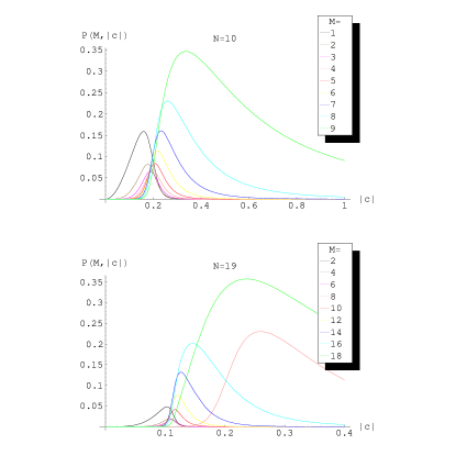
Figure 1: (Color online) The probability $P(M,c)$ for obtaining the Dicke state $\left|M,N\right\rangle_{D}$ as a function of the amplitude of the coupling coefficient $\left|c\right|$. We consider two ensembles consisting of $N=10$ and $N=19$ atoms, and a different number of excitations $M$.

IV.2 Construction of the GHZ state of an atomic ensemble

We begin with the observation that the state Eq.(21), corresponding to the lowest possible order of entanglement between the individual atoms and the cavity field, may still yield a highly entangled state of the atomic ensemble after being projected onto a linear combination of the field vacuum and a highly excited Fock state. Let us take the linear-combination field state

$$\left|F\right\rangle=B\left|0\right\rangle_{p}+C\left|N\right\rangle_{p},$$ (24)

where $N$ is the total number of atoms. Then this projection can be shown to result in the GHZ state. In fact, by casting Eq.(21) in the Taylor series

$$\left|\Psi\right\rangle=\frac{1}{A}\overset{N}{\underset{n=1}{{\displaystyle\sum}}}\frac{\left(\widehat{a}\dagger\right)^{n}}{n!}\left(\sum\limits_{n=1}^{N}\widehat{\sigma}_{n}^{+}I_{n}\right)^{n}\left|\mathcal{O}\right\rangle$$ (25)

one immediately finds the projection

$$\left\langle F\right.\left|\Psi\right\rangle =\frac{1}{A}\left[B^{\ast}+\frac{C^{\ast}}{\sqrt{N!}}\left(\sum\limits_{n=1}^{N}\widehat{\sigma}_{n}^{+}I_{n}\right)^{N}\right]\left|\emph{O}\right\rangle$$

$$=\left(\frac{B^{\ast}}{A}+\frac{C^{\ast}}{A\sqrt{N!}}\prod\limits_{n=1}^{N}\widehat{\sigma}_{n}^{+}I_{n}\right)\left|\emph{O}\right\rangle,$$ (26a)

For

$$B^{\ast}\sqrt{N!}=C^{\ast}\prod\limits_{n=1}^{N}I_{n},$$ (26b)

this indeed yields the GHZ state with the tanglemeter $$f_{GHZ}$$ of Eq.(20b).

Detection of the field state $\left|F\right\rangle$ cannot however be directly performed as a probabilistic projection on the photon number basis and requires a manipulation of the field prior to such a measurement. One way to perform such a manipulation is to expose the system to the Kerr-nonlinear interaction Eq.(19) with the parameters chosen such that only the corresponding states with $0$ and $N$ cavity photons are resonant and coupled. This condition reads

$$\left(\omega_{c}-\omega_{L}\right)N+\kappa N^{2}=0,$$ (27)

while the corresponding matrix element of the multiphoton transition between the photon vacuum and $N$-th Fock state has the form

$$V_{0N}=\frac{\left(\kappa\mathcal{E}^{3}\right)^{N}\sqrt{N!}}{\overset{N}{\underset{n=1}{{\textstyle\prod}}}\left(\kappa n^{2}-\omega_{L}n\right)}=\frac{\mathcal{E}^{3N}}{\sqrt{N!}\overset{N}{\underset{n=1}{{\textstyle\prod}}}\left(n-\omega_{L}/\kappa\right)}.$$ (28)

The interaction Eq.(19) must be on during a time $t_{Kerr}$, given by the condition

$$\tan\left(t_{Kerr}V_{0N}\right)=\frac{C^{\ast}}{B^{\ast}}=\sqrt{N!}/\prod\limits_{n=1}^{N}I_{n},$$ (29)

Then, if the cavity field is detected in the vacuum state, the projection onto the state $\left|F\right\rangle$ is performed. This results in the GHZ multiatomic state.

IV.3 Entangling two ensembles

We now consider entanglement between two ensembles of atoms, $A$ and $B$, each consisting of $N$ identical atoms. Each ensemble is treated as a single element and we are exclusively concerned with the collective entanglement between these multiatomic elements expressed in terms of the collective operators $\widehat{\sigma}_{A}^{+}=\sum\limits_{n=1}^{N}\widehat{\sigma}_{n}^{\left(A\right)+}$ and $\widehat{\sigma}_{B}^{+}=\sum\limits_{n=1}^{N}\widehat{\sigma}_{n}^{\left(B\right)+}.$ We guide the first ensemble of atoms through the cavity and then repeat the procedure for the second ensemble. If the excitation per atom remains small and the cavity is tuned on resonance with the atoms frequency, then according to Eq.(9) the combined state of the two multiatomic ensembles and the cavity field reads

$$\left|\Psi\right\rangle=\frac{1}{A}\mathrm{e}^{\mu\widehat{a}\dagger\left(\widehat{\sigma}_{A}^{+}+\widehat{\sigma}_{B}^{+}\right)}\left|\mathcal{O}\right\rangle\ .$$ (30)

Entanglement between the two ensembles is implied by the presence of cross terms $\left(\widehat{\sigma}_{A}^{+}\right)^{k}\left(\widehat{\sigma}_{B}^{+}\right)^{l}$ in the nilpotential, can appear as a result of the field manipulation prior to the measurement of the cavity photon number. In accordance with the results of Sect.III, the lowest-order cross term with $k=l=1$ can be generated from the state Eq.(30), by squeezing the cavity field followed by the detection of the cavity vacuum. More specifically, after the squeezing operator $S=\exp\left(g\widehat{\alpha}^{2}-g\widehat{\alpha}^{\dagger 2}\right)$ has been applied to the state Eq.(30) for time $t$, and zero photons are detected, the ensemble state adopts the form

$$\left|\Phi\right\rangle=\frac{r}{A^{\prime}}\exp(\zeta\widehat{O}^{2}+\eta)\left|\emph{O}\right\rangle\ ,$$ (31a)

where

$$\widehat{O} =\mu\left(\widehat{\sigma}_{A}^{+}+\widehat{\sigma}_{B}^{+}\right)\ ,$$

$$r =\frac{\sqrt{2\pi}}{\sqrt{1+e^{2gt}}},\;\eta=gt,\;\zeta=2\tanh[gt]-gt\;,$$ (31b)

and the value of the parameter $$\mu$$, given by Eq.(10), is identical for all the atoms.

V Discussion

We have presented a powerful formalism for the analytical description of multiatomic ensembles interacting with quantized cavity fields for the case where the atoms have low excitation probability and the effect of decoherence is ignored. By combining the analytical functional integration with the multipartite entanglement description via nilpotent polynomials we have been able to propose general schemes for the probabilistic control of entanglement among multiple neutral atoms. These techniques consist of manipulations on the cavity field followed by a projective measurement on the photon number state and therefore are experimentally feasible only in optical cavities. We presented several applications in the regime where the frequency of the cavity mode is resonant with the atomic transition frequency.

The proposed control scheme presumes the resolution of various experimental problems posed by state preparation and detection, most importantly the determination of atom number $N$ in the cavity. There is continuing progress towards the measurement of trapped atom numbers, suggesting that this goal may be achieved before long. The following procedure may be conceived of: (i) slowly trapping ground-state atoms in the cavity (for which several options exist, including the adiabatic conveyor - belt technique Merschede ); (ii) counting the trapped atoms by their resonance fluorescence or other optical techniques; (iii) impressing Stark or Zeeman shifts to make atoms at different positions spectrally distinguishable and thus addressable by the control Raman coupling; (iv) switching (on and off) the Raman control field in Hamiltonian (1) for selected (spectrally addressable ) atoms for the required interaction time. This procedure, although challenging, may in the long run allow field - atom entangling manipulations without actually sending atoms in and out of the cavity, but rather making them disappear and reappear by purely optical manipulations.

Beyond the ability to realize a broader variety of entangled multiatom states than existing states, the main merit of the present analysis is that it has been exhibited within the unified framework of the general nilpotent formalism.

VI Acknowledgements

This work is supported in part by the EC RTN QUACS. A.M. gratefully acknowledges Ile de France for financial support. G.K. acknowledges the support of the EC NOE SCALA, ISF and GIF.

Appendix A Functional integration

The straightforward way to calculate the functional integral of Eq.(8) is by transforming it into a Gaussian functional integral. This requires first to find the stationary solutions $z_{s}^{\ast}(\tau)$, $z_{s}(\tau)$ that correspond to the extremum of the functional exponent, i.e., the action $S$,

$$S =-\mathrm{i}\int\limits_{0}^{t}\left|z(\tau)\right|^{2}\mathrm{d}\tau+\mathrm{i}\sum\limits_{n=1}^{N}\frac{\omega_{n}}{2}t$$

$$-\mathrm{i}\sum\limits_{n=1}^{N}\widehat{\sigma}_{n}^{+}\int\limits_{0}^{t}\mathrm{e}^{\mathrm{i}\omega_{n}\left(\tau-t\right)}C_{n}\left(\tau\right)z(\tau)\mathrm{d}\tau$$

$$+\mathrm{i}\widehat{a}\dagger\int\limits_{0}^{t}\mathrm{e}^{\mathrm{i}\omega_{0}(\tau-t)}\mathcal{E}(\tau)z^{\ast}(\tau)\mathrm{d}\tau$$

$$-\int\limits_{0}^{t}\int\limits_{\tau}^{t}\mathrm{e}^{\mathrm{i}\omega_{0}(\tau-\theta)}\mathcal{E}(\tau)\mathcal{E}(\theta)z^{\ast}(\tau)z^{\ast}(\theta)\mathrm{d}\tau\mathrm{d}\theta,$$ (32)

and then to evaluate the integral for new functional variables $\left\{z^{\ast}\left(\tau\right)+z_{s}^{\ast}(\tau),z\left(\tau\right)+z_{s}(\tau)\right\}$.

By variation of the action $S$

$$0 =\delta S=\int\limits_{0}^{t}\mathrm{d}\tau\left[-\mathrm{i}z^{\ast}(\tau)-\mathrm{i}\sum\limits_{n=1}^{N}\widehat{\sigma}_{n}^{+}C_{n}\left(\tau\right)\mathrm{e}^{-\mathrm{i}\omega_{n}\left(t-\tau\right)}\right]\delta z(\tau)$$

$$-\left[\mathrm{i}z(\tau)-\mathrm{i}\widehat{a}\dagger\mathrm{e}^{\mathrm{i}\omega_{0}(\tau-t)}\mathcal{E}(\tau)+\mathcal{E}(\tau)\int\limits_{\tau}^{t}\mathrm{e}^{\mathrm{i}\omega_{0}(\tau-\theta)}\mathcal{E}(\theta)z^{\ast}(\theta)\mathrm{d}\theta+\mathcal{E}(\tau)\int\limits_{0}^{\tau}\mathcal{E}(\theta)z^{\ast}(\theta)\mathrm{e}^{\mathrm{i}\omega_{0}(\theta-\tau)}\mathrm{d}\theta\right]\delta z^{\ast}(\tau)$$ (33)

one obtains the stationary solutions

$$z_{s}^{\ast}(\tau) =\mathrm{-}\sum\limits_{n=1}^{N}\widehat{\sigma}_{n}^{+}C_{n}\left(\tau\right)\mathrm{e}^{-\mathrm{i}\omega_{n}\left(t-\tau\right)}$$

$$z_{s}(\tau) =\widehat{a}\dagger\mathrm{e}^{\mathrm{i}\omega_{0}(\tau-t)}\mathcal{E}(\tau)$$

$$-\mathrm{i}\sum\limits_{n=1}^{N}\widehat{\sigma}_{n}^{+}\mathcal{E}(\tau)\left(\int\limits_{\tau}^{t}\mathcal{E}(\theta)C_{n}\left(\theta\right)\mathrm{e}^{-\mathrm{i}\omega_{n}\left(t-\theta\right)+\mathrm{i}\omega_{0}(\tau-\theta)}\mathrm{d}\theta+\int\limits_{0}^{\tau}\mathcal{E}(\theta)C_{n}\left(\theta\right)\mathrm{e}^{-\mathrm{i}\omega_{n}\left(t-\theta\right)+\mathrm{i}\omega_{0}(\theta-\tau)}\mathrm{d}\theta\right).\vskip 3.0pt plus 1.0pt minus 1.0pt$$ (34)

The substitution of the new variables into Eq.(32), separates the action $S$ into two parts

$$S=S(z\left(\tau\right),z^{\ast}\left(\tau\right))+S(z_{s}\left(\tau\right),z_{s}^{\ast}\left(\tau\right)),$$ (35)

a “quantum”  part and a “classical” one. The quantum contribution of the action does not contain quantum operators in our case and the functional integration over this gives just a phase that can be ignored. What is left then is to evaluate the classical contribution to the functional integral by substituting  $S_{cl}=S(z_{s}\left(\tau\right),z_{s}^{\ast}\left(\tau\right))$

$$S_{cl} =\mathrm{i}\sum\limits_{n=1}^{N}\frac{\omega_{n}}{2}t-\mathrm{i}\widehat{a}\dagger\sum\limits_{n=1}^{N}\widehat{\sigma}_{n}^{+}\int\limits_{0}^{t}\mathrm{e}^{\mathrm{i}\left(\omega_{0}+\omega_{n}\right)(\tau-t)}C_{n}\left(\tau\right)\mathcal{E}(\tau)\mathrm{d}\tau$$

$$+\sum\limits_{n,m=1}^{N}\widehat{\sigma}_{n}^{+}\widehat{\sigma}_{m}^{+}\int\limits_{0}^{t}\int\limits_{0}^{\tau}\mathcal{E}(\tau)\mathcal{E}(\theta)C_{n}\left(\theta\right)C_{m}\left(\tau\right)\mathrm{e}^{-\mathrm{i}\left(\tau(\omega_{0}-\omega_{m}\right)+t(\omega_{n}+\omega_{m)}-\theta(\omega_{n}+\omega_{0}))}\mathrm{d}\theta\mathrm{d}\tau.$$ (36)

into Eq.(8). The final expression for the wave function describing the time-evolution of the combined cavity-atoms state is

$$\left|\Psi\left(t\right)\right\rangle =\frac{1}{A(t)}\exp\left[\mathrm{i}\sum\limits_{n=1}^{N}\frac{\omega_{n}}{2}t+\mathrm{i}\widehat{a}\dagger\sum\limits_{n=1}^{N}\widehat{\sigma}_{n}^{+}\int\limits_{0}^{t}\mathrm{e}^{\mathrm{i}\left(\omega_{0}+\omega_{n}\right)(\tau-t)}C_{n}\left(\tau\right)\mathcal{E}(\tau)\mathrm{d}\tau\right]$$

$$\exp\left[+\sum\limits_{n,m=1}^{N}\widehat{\sigma}_{n}^{+}\widehat{\sigma}_{m}^{+}\int\limits_{0}^{t}\int\limits_{0}^{\tau}\mathcal{E}(\tau)\mathcal{E}(\theta)C_{n}\left(\theta\right)C_{m}\left(\tau\right)\mathrm{e}^{-\mathrm{i}\left(\tau(\omega_{0}-\omega_{m}\right)+t(\omega_{n}+\omega_{m)}-\theta(\omega_{n}+\omega_{0}))}\mathrm{d}\theta\mathrm{d}\tau\right]\left|\mathcal{O}\right\rangle.$$ (37)

where $A(t)$ is the normalization factor whose derivation is presented in the following.

A.1 Normalization factor

By definition the square of the normalization factor, using the notation of Eqs.(9)-(11), is

$$\left|A(t)\right|^{2}=\left\langle\mathcal{O}\right|\exp\left[\widehat{a}\sum\limits_{n=1}^{N}\widehat{\sigma}_{n}^{-}I_{n}^{\ast}+\sum\limits_{n,m=1}^{N}\widehat{\sigma}_{n}^{-}\widehat{\sigma}_{m}^{-}I_{m,n}^{\ast}\right]\exp\left[\widehat{a}\dagger\sum\limits_{n=1}^{N}\widehat{\sigma}_{n}^{+}I_{n}+\sum\limits_{n,m=1}^{N}\widehat{\sigma}_{n}^{+}\widehat{\sigma}_{m}^{+}I_{n,m}\right]\left|\mathcal{O}\right\rangle,$$ (38)

or, equivalently, after expanding the terms involving the operators $\widehat{a}$ and $\widehat{a}\dagger$,

$$\left|A(t)\right|^{2}=\left\langle\emph{O}\right|\exp\left[\sum\limits_{n,m=1}^{N}\widehat{\sigma}_{n}^{-}\widehat{\sigma}_{m}^{-}I_{m,n}^{\ast}\right]\exp\left[\sum\limits_{n=1}^{N}\widehat{\sigma}_{n}^{-}I_{n}^{\ast}\sum\limits_{m=1}^{N}\widehat{\sigma}_{m}^{+}I_{m}\right]\exp\left[\sum\limits_{n,m=1}^{N}\widehat{\sigma}_{n}^{+}\widehat{\sigma}_{m}^{+}I_{n,m}\right]\left|\emph{O}\right\rangle.$$ (39)

Under the assumption of low excitation probability per atom, the collective operators approximately commute and the Eq.(39) may be rewritten in the form

$$\left|A(t)\right|^{2}\simeq\left\langle\emph{O}\right|\exp\left[\sum\limits_{n,m=1}^{N}\widehat{\sigma}_{n}^{-}\widehat{\sigma}_{m}^{-}I_{m,n}^{\ast}+\sum\limits_{n=1}^{N}\widehat{\sigma}^{-}I_{n}^{\ast}\sum\limits_{m=1}^{N}\widehat{\sigma}_{m}^{+}I_{m}+\sum\limits_{n,m=1}^{N}\widehat{\sigma}_{n}^{+}\widehat{\sigma}_{m}^{+}I_{n,m}\right]\left|\emph{O}\right\rangle.$$ (40)

The expression  (40) can be written in a simpler way as

$$\left|A(t)\right|^{2}=\left\langle\emph{O}\right|\exp\left[\overline{y}My\right]\left|\emph{O}\right\rangle,$$ (41)

by introducing a Hermitian matrix $M$ and  a complex vector $y$

$$M=\left(\begin{tabular}[c]{cccccc}$\frac{1}{2}I_{1}I_{1}^{\ast}$&\ldots&$\frac{1}{2}I_{1}I_{N}^{\ast}$&$I_{1,1}$&\ldots&$I_{1,N}$\\ $\vdots$&$\ddots$&$\vdots$&$\vdots$&$\ddots$&$\vdots$\\ $\frac{1}{2}I_{N}I_{1}^{\ast}$&\ldots&$\frac{1}{2}I_{N}I_{N}^{\ast}$&$I_{N,1}$&\ldots&$I_{1,N}$\\ $I_{1,1}^{\ast}$&\ldots&$I_{N,1}^{\ast}$&$\frac{1}{2}I_{1}I_{1}^{\ast}$&\ldots&$\frac{1}{2}I_{N}I_{1}^{\ast}$\\ $\vdots$&$\ddots$&$\vdots$&$\vdots$&$\ddots$&$\vdots$\\ $I_{1,N}^{\ast}$&\ldots&$I_{1,N}^{\ast}$&$\frac{1}{2}I_{1}I_{N}^{\ast}$&\ldots&$\frac{1}{2}I_{N}I_{N}^{\ast}$\end{tabular}\ \ \ \ \right),y=\left(\begin{tabular}[c]{c}$\sigma_{1}^{-}$\\ $\vdots$\\ $\sigma_{N}^{-}$\\ $\sigma_{1}^{+}$\\ $\vdots$\\ $\sigma_{N}^{+}$\end{tabular}\ \ \ \ \right).$$ (42)

At this point, we can employ the identity

$${\displaystyle\int}dx^{N}d\overline{x}^{N}\exp\left[-\left(\overline{x+w}\right)A(x+w)\right]=\frac{\left(2\pi\right)^{N}}{\det A}$$ (43)

that holds for complex vectors $x$ and $w$, to prove that

$$e^{\overline{z}A^{-1}z}=\frac{\det A}{\left(2\pi\right)^{N}}{\displaystyle\int}dx^{N}d\overline{x}^{N}\exp\left[-\overline{x}Ax-\overline{z}x-\overline{x}z\right]\ ,$$ (44)

for $A$, a Hermitian matrix and $z$, a vector defined as $z=Aw$.

With the help of the identity (44) we can rewrite Eq.(41) as

$$\left|A(t)\right|^{2} =\left\langle\emph{O}\right|\exp\left[\overline{y}My\right]\left|\emph{O}\right\rangle$$

$$=\frac{\det M^{-1}}{\left(2\pi\right)^{2N}}{\displaystyle\int}dx^{2N}d\overline{x}^{2N}\left\langle\emph{O}\right|\exp\left[-\overline{x}M^{-1}x-\overline{y}x-\overline{x}y\right]\left|\emph{O}\right\rangle$$

$$\simeq\frac{\det M^{-1}}{\left(2\pi\right)^{2N}}{\displaystyle\int}dx^{2N}d\overline{x}^{2N}\exp\left[-\overline{x}M^{-1}x+\left(x+\overline{x}\right)V\left(x+\overline{x}\right)\right]$$

$$=\frac{\det M^{-1}}{\left(2\pi\right)^{2N}}{\displaystyle\int}dx^{2N}d\overline{x}^{2N}\exp\left[-\left(\begin{array}[c]{cc}x&\overline{x}\end{array}\right)B\left(\begin{array}[c]{c}\overline{x}\\ x\end{array}\right)\right]$$ (48)

$$=\frac{\det M^{-1}}{\det B}\ ,$$ (49)

where we have assumed that $x_{i}$ small, an assumption valid in the chosen regime, and

$$V=\left(\begin{array}[c]{cc}0&I_{2N}\\ I_{2N}&0\end{array}\right),\ \ B=\left(\begin{array}[c]{cc}V&V\\ V&V-M^{-1}\end{array}\right)\;.$$ (50)

Appendix B Squeezing operators

Having projected the squeezed state onto the vacuum

$$\left|\Phi\right\rangle=\left\langle 0_{p}\right|\mathrm{e}^{\left(g\left(\widehat{\alpha}+\widehat{O}\right)^{2}-g^{\ast}\widehat{\alpha}^{\dagger 2}\right)t}\left|0_{p}\right\rangle\mathrm{e}^{\widehat{G}}\left|\emph{O}\right\rangle$$ (51)

we would like to explicitly calculate the state of the atoms in the special case where $g=g^{\ast}$.  If the position-momentum representation of the ladder operations is employed,

$$\widehat{\alpha} =\frac{1}{\sqrt{2}}(\widehat{x}+\frac{\partial}{\partial\widehat{x}}),$$

$$\widehat{\alpha}^{\dagger} =\frac{1}{\sqrt{2}}(\widehat{x}-\frac{\partial}{\partial\widehat{x}})$$ (52)

the problem is reduced in solving the Shrödinger equation for the Hamiltonian

$$\widehat{H} =i\left(g\left(\widehat{\alpha}+\widehat{O}\right)^{2}-g\widehat{\alpha}^{\dagger 2}\right)$$

$$=i\left(\sqrt{2}g\widehat{O}+g\widehat{x}\right)\frac{\partial}{\partial\widehat{x}}+i\left(\sqrt{2}g\widehat{O}\widehat{x}+g+g\widehat{O}^{2}\right)$$ (53)

and with initial condition

$$\left\langle x|0_{p}\right\rangle=e^{-x^{2}/2}.$$ (54)

If $g$ is a real number, the differential equation to be solved is of first order both in position and time and thus can be easily handled. The final result is

$$\left|\Phi\right\rangle=r\exp\left[\zeta\widehat{O}^{2}+\eta\right]\exp\left[\widehat{G}\right]\left|\emph{O}\right\rangle$$ (55)

where $t$ is time period that the squeezing operator is applied and the parameters are

$$r=\sqrt{2\pi}/\sqrt{1+e^{2gt}},~{}~{}\eta=gt,~{}~{}\zeta=2\tanh[gt]-gt.$$ (56)

References

- (1) L. -M. Duan and H. J. Kimble, Phys. Rev. Let. 90, 253601 (2003).
- (2) C. Marr, A. Beige, and G. Rempe, Phys. Rev. A 68, 033817 (2003).
- (3) J. M. Raimond, M. Brune, and S. Haroche, Rev. Mod. Phys. 73, 565 (2001).
- (4) C. Schön, E. Solano, F. Verstaete, J. I. Cirac, and M. M. Wolf, Phys. Rev. Lett. 95, 110503 (2005).
- (5) D. Jaksch, H.-J. Briegel, J.I. Cirac, C. W. Gardiner, P. Zoller, Phys.Rev.Lett. 82, 1975-1978 (1999); O. Mandel, M. Greiner, A. Widera, T. Rom, T. W. Hänsch and I. Bloch, Nat. 425, 937-940 (2003); T. Opatrny, B. Deb, G. Kurizki, Phys. Rev. Lett. 90, 250404 (2003);
- (6) K. Mølmer and A. Sørensen, Phys. Rev. Lett. 82, 1835 (1999); C.A. Sackett et al., Nat. 404, 256 (2000); R. G. Unanyan, M. Fleischhauer, N. V. Vitanov, K. Bergmann, Phys. Rev. A 66, 042101 (2002); H. Haeffner et al., Nat. 438, 643-646 (2005); J. J. Garcia-Ripoll, P. Zoller, J. I. Cirac, Phys. Rev. A 71, 062309 (2005).
- (7) A. Mandilara, V. M. Akulin, A. V. Smilga and L. Viola, Phys. Rev. A 74, 022331 (2006).
- (8) R. H. Dicke, Phys. Rev. 93, 99 (1954).
- (9) W. Dur, G. Vidal, and J. I. Cirac, Phys. Rev. A. 62, 062314 (2000); L.-B. Fu, J.-L. Chen, and X.-G. Zhao, Phys. Rev. A 68, 022323 (2003).
- (10) D. M. Greenberger, M. Horne and A. Zeilinger, M. Kafatos Ed., (Kluwer, Dordrecht, 1989), pp.69-72.
- (11) H. Barnum, E. Knill, G. Ortiz, R. Somma, L. Viola, Phys. Rev. Lett. 92, 107902 (2004); H. Barnum, E. Knill, G. Ortiz, and L. Viola, Phys. Rev. A 68, 032308 (2003).
- (12) D. Schrader, I. Dotsenko, M. Khudaverdyan, Y. Miroshnychenko, A. Rauschenbeutel, and D. Meschede, Phys. Rev. Lett. 93, 150501 (2004).
- (13) A. S. Sørensen and Klaus Mølmer, Phys. Rev. Lett. 90, 127903 (2003).
- (14) M. B. Plenio, S. F. Huelga, A. Beige, and P. L. Knight, Phys. Rev. A 59, 2468 (1999).
- (15) C. W. Chou et al., Nat. 438, 828 (2005).
- (16) V. Coffman, J. Kundu and W. K. Wootters, Phys. Rev. A 61, 052306 (2000).
- (17) F. Verstraete, J. Dehaene, B. DeMoor, and H. Verschelde, Phys. Rev. A 65, 052112 (2002).
- (18) M. O. Scully and M. S. Zubairy, Quantum Optics, Cambridge University Press (1997).
- (19) F. Verstraete, J. Dehaene, and B. De Moor, Phys. Rev. A 68, 012103 (2003).
- (20) L. -M. Duan, M. D. Lukin, J. I. Cirac and P. Zoller, Nat. 414, 413 (2001); M. D. Lukin, Rev. Mod. Phys. 75, 457-472 (2003); A. Dantan, N. Treps, A. Bramati and M. Pinard Phys. Rev. Lett. 94, 050502 (2005); M. D. Lukin, S. F. Yulin and M. Fleischhauer, Phys. Rev. Lett. 84, 4232 (2000).