Gaussian Decoherence and Gaussian Echo from Spin Environments

Abstract

We examine an exactly solvable model of decoherence – a spin-system interacting with a collection of environment spins. We show that in this simple model (introduced some time ago to illustrate environment–induced superselection) generic assumptions about the coupling strengths typically lead to a non-Markovian (Gaussian) suppression of coherence between pointer states. We explore the regime of validity of this result and discuss its relation to spectral features of the environment. We also consider its relevance to Loschmidt echo experiments (which measure, in effect, the fidelity between the initial state and the state first evolved forward with a Hamiltonian ${\cal H}$, and then “unevolved” with (approximately) $-{\cal H}$). In particular, we show that for partial reversals (e.g., when only a part of the total Hamiltonian changes sign) fidelity may exhibit a Gaussian dependence on the time of reversal that is independent of the details of the reversal procedure: It just depends on what part of the Hamiltonian gets “flipped” by the reversal. This puzzling behavior was observed in several NMR experiments. Natural candidates for such two environments (one of which is easily reversed, while the other is “irreversible”) are suggested for the experiment involving ferrocene.

I Introduction

“It seems very important to us… that the idea and genesis of randomness can be made rigorously precise also if one rigorously follows the determinism; the law of large numbers comes then not as a mystical principle and not as a purely empirical fact, but as a simple mathematical result…” wrote Marian Smoluchowski in his posthumously published paper Smol1918 . At that time determinism meant classical determinism – the underlying equations of motion that determined a trajectory of a classical particle. One could, however, develop simple stochastic models that encapsulated effects of that exact dynamics. That was the essence of the approach that led to the Smoluchowski equation (which is still widely used today, a century after it was derived using this strategy).

Quantum theory forces one to reassess the relation between determinism and randomness: Chance plays a different role in the quantum domain. According to Bohr and Born, quantum randomness is fundamental: A measurement on a quantum system – according to the Copenhagen interpretation – necessarily involves a classical apparatus. The outcome of the measurement is randomly selected with probability given by the famous rule that connects probability to amplitude ($p_{k}=|\psi_{k}|^{2}$) conjectured by Max Born. The Copenhagen view of the quantum Universe was challenged by Everett, who half a century ago noted that it is possible to imagine that our Universe is all quantum, and that its global evolution is deterministic. Randomness will appear only as a result of the local nature of subsystems (such as an apparatus or an observer) Zurek82 ; Zurek03 .

It is not our aim here to recapitulate this well known story, except to point out that it sheds a rather different light on the relation between determinism and randomness than did classical physics. The key insight of Smoluchowski contained in the quote above is, however, still correct – perhaps even more deeply correct – in the quantum setting. Entanglement, the quintessential quantum phenomenon, which plays such an important role in the approach of Everett is central for its validity. We illustrate here only one aspect of these connections – decoherence which is caused by entangling interactions between the system and the environment.

The story that will unfold makes one more connection with Smoluchowski: It touches on the debate about the origins and nature of irreversibility between his two former professors – Boltzmann and Loschmidt – as the evolution responsible for the buildup of correlations which lead to decoherence can be (approximately) reversed in suitable settings, allowing for the study of “Loschmidt echo” horaciobook ; horacioexponential ; horaciosaturation ; horaciodifusion .

II Spin Decoherence Model

A single spin–system ${\cal S}$ (with states $\left\{\left|0\right>,\left|1\right>\right\}$) interacting with an environment ${\cal E}$ of many independent spins ($\left\{\left|\uparrow_{k}\right>,\left|\downarrow_{k}\right>\right\}$, $k=1..N$) through the Hamiltonian

$${\cal H_{SE}}=\left(\left|0\right>\left<0\right|-\left|1\right>\left<1\right|\right)\sum_{k=1}^{N}\frac{g_{k}}{2}\left(\left|\uparrow_{k}\right>\left<\uparrow_{k}\right|-\left|\downarrow_{k}\right>\left<\downarrow_{k}\right|\right)$$ (1)

may be the simplest solvable model of decoherence. It was introduced some time ago Zurek82 to show that relatively straightforward assumptions about the dynamics can lead to the emergence of a preferred set of pointer states due to einselection (environment–induced superselection) Zurek82 ; deco . Such models have gained additional importance in the past decade because of their relevance to quantum information processing spindeco .

The purpose of our paper is to show that – with a few additional natural and simple assumptions – one can evaluate the exact time dependence of the reduced density matrix, and demonstrate that the off–diagonal components display a Gaussian (rather than exponential) decay ZCP . In effect, we exhibit a simple soluble example of a situation where the usual Markovian Kossakowski assumptions about the evolution of a quantum open system are not satisfied. Apart from their implications for decoherence, our results are also relevant to quantum error correction ErrorCorrection where precise precise knowledge of the dynamics is essential to select an efficient strategy. Moreover, while the model Hamiltonian of Eq. (1) is very specific, it suggests generalizations that lead one to conclude that Gaussian decay of polarization may be common, and specify when a reversal of the Hamiltonian evolution in a part of the spin environment naturally leads to a Gaussian dependence of the return signal on the time of reversal, a feature of Loschmidt echo observed in NMR experiments.

To demonstrate the Gaussian time dependence of decoherence we first write down a general solution for the model given by Eq. (1). Starting with:

$$\left|\Psi_{\cal SE}(0)\right>=(a\left|0\right>+b\left|1\right>)\bigotimes_{k=1}^{N}\left(\alpha_{k}\left|\uparrow_{k}\right>+\beta_{k}\left|\downarrow_{k}\right>\right),$$ (2)

the state of ${\cal SE}$ at an arbitrary time is given by:

$$\left|\Psi_{\cal SE}(t)\right>=a\left|0\right>\left|{\cal E}_{0}(t)\right>+b\left|1\right>\left|{\cal E}_{1}(t)\right>$$ (3)

where

$$\left|{\cal E}_{0}(t)\right> = \bigotimes_{k=1}^{N}\left(\alpha_{k}e^{ig_{k}t/2}\left|\uparrow_{k}\right>+\beta_{k}e^{-ig_{k}t/2}\left|\downarrow_{k}\right>\right)$$ (4)

$$= \left|{\cal E}_{1}(-t)\right>.$$

The reduced density matrix of the system is then:

$$\rho_{\cal S} = {\rm Tr}_{\cal E}\left|\Psi_{\cal SE}(t)\right>\left<\Psi_{\cal SE}(t)\right|$$ (5)

$$= |a|^{2}\left|0\right>\left<0\right|+ab^{*}r(t)\left|0\right>\left<1\right|$$

$$+ a^{*}br^{*}(t)\left|1\right>\left<0\right|+|b|^{2}\left|1\right>\left<1\right|,$$

where the decoherence factor $r(t)=\left<{\cal E}_{1}(t)|{\cal E}_{0}(t)\right>$ can be readily obtained:

$$r(t) = \prod_{k=1}^{N}\left(|\alpha_{k}|^{2}e^{ig_{k}t}+|\beta_{k}|^{2}e^{-ig_{k}t}\right).$$ (6)

It is straightforward to see that $r(0)=1$, and that for $t>0$ it will decay to zero, so that the typical fluctuations of the off-diagonal terms of $\rho_{\cal S}$ will be small for large environments, since:

$$\left<|r(t)|^{2}\right>=2^{-N}\prod_{k=1}^{N}\left(1+(|\alpha_{k}|^{2}-|\beta_{k}|^{2})^{2}\right),$$ (7)

Here $\left<...\right>$ denotes a long time average Zurek82 . Clearly, $\left<|r(t)|^{2}\right>\underset{N\rightarrow\infty}{\longrightarrow}0$, leaving $\rho_{\cal S}$ approximately diagonal in a mixture of the pointer states $\left\{\left|0\right>,\left|1\right>\right\}$ which retain preexisting classical correlations.

This much was known since Zurek82 . The aim of this paper is to show that, for a fairly generic set of assumptions, the form of $r(t)$ can be further evaluated and that – quite universally – it turns out to be approximately Gaussian in time. Thus, the simple model of Ref. Zurek82, predicts a universal (Gaussian) form of the loss of quantum coherence, whenever the couplings $g_{k}$ of Eq. (1) are sufficiently concentrated near their average value so that their standard deviation $\left<(g_{k}-\left<g_{k}\right>)^{2}\right>$ exists and is finite. When this condition is not fulfilled other sorts of time dependence become possible. In particular, $r(t)$ may be exponential when the distribution of couplings is a Lorentzian.

We shall also consider implications of the predicted time dependence of $r(t)$ for echo experiments. In particular, the group of Levstein and Pastawski horaciobook ; horacioexponential ; horaciodifusion ; horaciosaturation , have carried out experiments that aim to implement time reversal of dynamics, as was suggested long time ago by Loschmidt loschmidt , who used time reversal as a counterargument to Boltzmann’s ideas about H-theorem and the origins of irreversibility. Boltzmann’s reported (possibly apocryphal) reply “Go ahead and do it!”, which may reflect his belief in the molecular disorder hypothesis kuhn , points to the origin of the difficulty in implementing such reversal in practice for all of the relevant degrees of freedom. It is nevertheless possible in some settings to carry out “Loschmidt echo experiments” that approximate Loschmidt’s original idea loschmidt .

When the reversal is successful for only some of the relevant degrees of freedom (${\cal E}^{\prime\prime}$) but does not encompass all of the environment ${\cal E}$ (leaving behind “unreversed” ${\cal E}^{\prime}$) the result is a partial Loschmidt echo (also dubbed “Boltzmann echo” jacquod ). As in Ref. LEdeco , we interpret the decay in the Loschmidt echo as the effect of coupling to a second environment. We shall study the partial Loschmidt echo in the context of the simple model of Eq. (1) and Ref. Zurek82 , and conclude that its basic implications may generalize to a much broader range of dynamics relevant to NMR experiments.

In our case the state of all the degrees of freedom after a partial reversal (that happens at $t=t_{R}$) is given by:

$$|\Phi_{{\cal S}{\cal E}^{\prime}{\cal E}^{\prime\prime}}(t)\rangle=e^{iH_{{\cal S}{\cal E}^{\prime}}t}e^{iH_{{\cal S}{\cal E}^{\prime\prime}}(2t_{R}-t)}|\Phi_{{\cal S}{\cal E}^{\prime}{\cal E}^{\prime\prime}}(0)\rangle$$ (8)

The echo signal measured in the experiments concerns only a part of the whole – the system ${\cal S}$. It is given by:

$$\mu(2t_{R})=Tr\rho_{\cal S}(t=0)\rho_{\cal S}(t=2t_{R})\ .$$

This is in effect the fidelity of the state of ${\cal S}$. We shall express $\mu(t)$ in terms of decoherence factors corresponding to ${\cal E}^{\prime}$ and ${\cal E}^{\prime\prime}$: This follows from a straightforward generalization of Eqs. (5, 6) to the case of partial Loschmidt echo with two environments, only one of which gets reversed.

III Gaussian Decoherence

Evaluating time dependence of the decoherence factors for ${\cal E}^{\prime}$ and ${\cal E}^{\prime\prime}$ is therefore our first goal. To this end we carry out multiplication of Eq.(6), re–expressing $r(t)$ as a sum:

$$r(t) = \prod_{k=1}^{N}|\alpha_{k}|^{2}e^{it\sum_{n}g_{n}}+\sum_{l=1}^{N}|\beta_{l}|^{2}\prod_{k\neq l}^{N}|\alpha_{k}|^{2}\times$$ (9)

$$e^{it(-g_{l}+\sum_{n\neq l}g_{n})}+\sum_{l=1}^{N}\sum_{m\neq l}^{N}|\beta_{l}|^{2}|\beta_{m}|^{2}\times$$

$$\prod_{k\neq l,m}^{N}|\alpha_{k}|^{2}e^{\left[it(-g_{l}-g_{m}+\sum_{n\neq l,m}^{N}g_{n})\right]}+...$$

Decoherence factor is then a sum of $2^{N}$ complex contributions with fixed absolute values and with phases that rotate at the rate given by the eigenvalues of the total Hamiltonian.

Decay of $r(t)$ can be understood (see Zurek82 ) as a progressive randomization of a walk in a complex plane: At $t=0$ all of the phases are the same so all of the steps – all of the contributions to the decoherence factor – add up in phase yielding $|r(t=0)|=1$. However, as time goes on, these phases rotate at various rates so $r(t)$ is a terminal point of what becomes in time a random walk (on a complex plane) where the directions of various steps are uncoordinated (see Fig. 1).

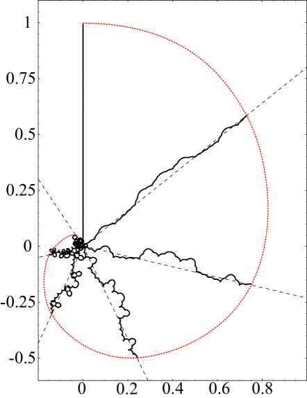
Figure 1: Decoherence factor $r(t)$ decomposed as a sum of complex terms as in Eq. (9), for $|\alpha_{k}|^{2}=|\beta_{k}|^{2}=1/2$ and $N=8$ spins in the environment with random couplings $g_{k}$ from a uniform distribution. The times plotted are $t=0$, (at “noon”), and $t=0.25$, $0.5$, $0.75$, $1$, $1.25$, and $1.5$ in a “clockwise direction”: The coordinate of the complex plane is rotated clockwise by an angle $2\pi/7$ for each $r(t)$ (dashed lines), starting with a vertical axis for $t=0$. Notice the random walk-like behavior of $r(t)$. The dotted curve line is the envelope of the random walks – the net decoherence factor decaying with a Gaussian form in accord with our discussion.

This view of the decay of $r(t)$ is the first instance where the random walk analogy is useful in our paper. The terminal point of this random walk determines decoherence factor. Another random walk – this time in energy – can be invoked in computing eigenvalues of the total Hamiltonian. These eigenvalues are responsible for the rotation rates of the individual steps that contribute to $r(t)$. We shall now see that this random walk in energies is responsible for the (typically Gaussian) decay of the decoherence factor.

To exhibit the Gaussian nature of $r(t)$ we start by noting that there are $\binom{N}{0}$, $\binom{N}{1}$, $\binom{N}{2}$, … etc. terms in the consecutive sums above. The binomial pattern is clear, and can be made even more apparent by assuming that $\alpha_{k}=\alpha$ and $g_{k}=g$ for all $k$. Then,

$$r(t)=\sum_{l=0}^{N}\binom{N}{l}|\alpha|^{2(N-l)}|\beta|^{2l}e^{ig(N-2l)t},$$ (10)

i.e., $r(t)$ is the binomial expansion of $r(t)=\left(|\alpha|^{2}e^{igt}+|\beta|^{2}e^{-igt}\right)^{N}$.

We now note that, as follows from the Laplace-de Moivre theorem Gnedenko , for sufficiently large $N$ the coefficients of the binomial expansion of Eq. (10) can be approximated by a Gaussian:

$$\binom{N}{l}|\alpha|^{2(N-l)}|\beta|^{2l}\simeq\frac{\exp{\left[-\frac{(l-N|\beta|^{2})^{2}}{2N|\alpha\beta|^{2}}\right]}}{\sqrt{2\pi N|\alpha\beta|^{2}}}.$$ (11)

This limiting form of the distribution of the eigenenergies of the composite ${\cal SE}$ system immediately yields our main result:

$$|r(t)|=\exp(-2N|\alpha\beta|^{2}(gt)^{2})$$ (12)

So, $r(t)$ is approximately Gaussian since it is a Fourier transform of an approximately Gaussian distribution of the eigenenergies of the total Hamiltonian resulting from all the possible combinations of the couplings with the environment.

A few quick comments on the above form of the decoherence factor may be in order: We note that in the limit of large $Ng^{2}$ it predicts “instantaneous” decay of quantum coherence. We also note that when $\alpha\beta=0$ the environment is incapable of decohering the system (as it is then in an eigenstate of the global Hamiltonian, so the “measurement-like evolution” that is at the heart of decoherence is impossible). Last but not least, we note that when the environment is mixed, decoherence will proceed unimpeded, and that it will be most efficient when the mixture is perfect – when $|\alpha|^{2}=|\beta|^{2}=\frac{1}{2}$.

IV Law of Large Numbers and Energies

To yield a Gaussian decay of $|r(t)|$, the set of all the resulting eigenenergies of the total Hamiltonian must have an (approximately) Gaussian distribution. This behavior is generic, a result of the law of large numbers Gnedenko : these energies can be thought of as the terminal points of an $N$–step random walk. The contribution of the $k$–th spin of the environment to the random energy is $+g$ or $-g$ with probability $|\alpha|^{2}$ or $|\beta|^{2}$ respectively (Fig. 2-a).

The same argument can be carried out in the more general case of Eq. (9). The “random walk” picture that yielded the distribution of the couplings remains valid (see Fig. 2-b). However, now the individual steps in the random walk are not all equal. Rather, they are given by the set $\left\{g_{k}\right\}$ (see Eq. 1) with each step $g_{k}$ taken just once in a given walk. There are $2^{N}$ such distinct random walks. This exponential proliferation of the contributing coupling energies allows one to anticipate rapid convergence to the universal Gaussian form of their distribution, and, therefore, of the decoherence factor $r(t)$.

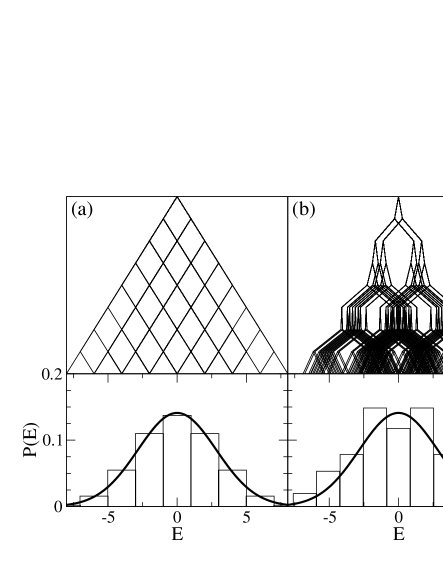
Figure 2: The distribution of the energies obtains from the random walks with the steps given by the coupling size and in the direction ($+g_{k}$ or $-g_{k}$) biased by the probabilities $|\alpha_{k}|^{2}$ and $|\beta_{k}|^{2}$ as in Eq. (17) (although in these examples we set $|\alpha_{k}|^{2}=1/2$). (a) When all the couplings have the same size $g_{k}=g$ (Eq. (10)), a simple Newton’s triangle leads to an approximate Gaussian for the distribution of energies. (b) When the couplings randomly differ from step to step (Eq. (9)), the resulting distribution still approaches an approximately Gaussian envelope for large $N$.

Indeed, we can regard eigenenergies resulting from the sums of $g_{k}$’s as a random variables. Its probability distribution is given by products of the corresponding weights. That is, the typical term in Eq. (9) is of the form:

$$p_{W}e^{iE_{W}t}\equiv\left(\prod_{k\in W^{+}}|\alpha_{k}|^{2}e^{ig_{k}t}\right)\left(\prod_{k\in W^{-}}|\beta_{k}|^{2}e^{-ig_{k}t}\right).$$ (13)

The resulting terminal energy is

$$E_{W}=\sum_{k\in W^{+}}g_{k}-\sum_{k\in W^{-}}g_{k},$$ (14)

and the cumulative weight $p_{W}$ is given by the corresponding product of $|\alpha_{k}|^{2}$ and $|\beta_{k}|^{2}$. Each such specific random walk $W$ corresponding to a given combination of right ($k\in W^{+}$) and left ($k\in W^{-}$) “steps” (see Figs. 1 and 2) contributes to the distribution of energies only once. The terminal points $E_{W}$ may or may not be degenerate: As seen in Fig. 2, in the degenerate case, the whole collection of $2^{N}$ random walks “collapses” into $N+1$ terminal energies. More typically, in the non-degenerate case (also displayed in Fig. 2), there are $2^{N}$ different terminal energies $E_{W}$. In both cases, the “envelope” of the distribution $P(E_{W})$ should be Gaussian, as we shall show below.

In contrast to the usual classical random walk scenario (where each event corresponds to specific random walk) in this quantum setting all of the random walks in the ensemble contribute simultaneously – evolution happens because the system is in a superposition of its energy eigenstates. The resulting decoherence factor $r(t)$ can be viewed as the characteristic function Gnedenko (i.e., the Fourier transform) of the distribution of eigenenergies $E_{W}$. Thus,

$$r(t)=\int e^{iEt}\eta(E)dE,$$ (15)

where the strength function $\eta(E)$, also known as the local density of states (LDOS) LDOS is defined in general as

$$\eta(E)=\sum_{\lambda}|\left<\Psi_{\cal SE}(0)|\phi_{\lambda}\right>|^{2}\delta(E-E_{\lambda}).$$ (16)

Above $\left|\phi_{\lambda}\right>$ are the eigenstates of the full Hamiltonian and $E_{\lambda}$ its eigenenergies. In our particular model (Eq. 1) the eigenstates are associated with all possible random walks in the set $W$, and therefore

$$\eta(E)=\sum_{W}p_{W}\delta(E-E_{W}).$$ (17)

Decoherence in our model is thus directly related to the characteristic function of the distribution of eigenenergies $\eta(E)$. Moreover, since the $E_{W}$’s are sums of $g_{k}$’s, $r(t)$ is itself a product of characteristic functions of the distributions of the couplings $\{g_{k}\}$, as we have already seen in the example of Eq. (6). Thus, the distribution of $E_{W}$ belongs to the class of the so–called infinitely divisible distributions Gnedenko ; breiman .

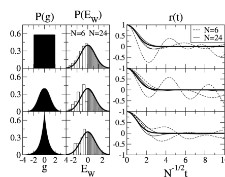
Figure 3: (Left panels) Assumed distribution of the couplings $g_{k}$, from top to bottom: uniform, Gaussian, and exponential. (Center panels) Resulting distribution of the eigenenergies $E_{W}$ (center panels) for $N=6$ ($E_{W}<0$) and $N=24$ ($E_{W}>0$). In the case of $|\alpha_{k}|^{2}=1/2$ this distribution is in effect the “strength function” (local density of states). (Right panels) Decoherence factor $r(t)$ for different initial conditions with $N=6$ (dashed lines), $N=24$ (thin solid lines) and the average (bold line) rapidly approaches a Gaussian whenever couplings have a finite variance.

The behavior of the decoherence factor $r(t)$ – characteristic function of an infinitely divisible distribution – depends only on the average and variance of the distributions of couplings weighted by the initial state of the environment Gnedenko ; breiman . The remaining task is to calculate $\eta(E)$, which can be obtained through the statistical analysis of the random walk picture described above. If we denote $x_{k}$ the random variable that takes the value $+g_{k}$ or $-g_{k}$ with probability $|\alpha_{k}|^{2}$ or $|\beta_{k}|^{2}$ respectively, then its mean value $a_{k}$ and its variance $b_{k}$ are

$$a_{k} = (|\alpha_{k}|^{2}-|\beta_{k}|^{2})g_{k},$$

$$b_{k}^{2} = g_{k}^{2}-a_{k}^{2}=4|\alpha_{k}|^{2}|\beta_{k}|^{2}g_{k}^{2}.$$ (18)

The behavior of the sums of $N$ random variables $x_{k}$ (and thus, of their characteristic function) depends on whether the so–called Lindeberg condition holds Gnedenko . It is expressed in terms of the cumulative variances $B_{N}^{2}=\sum b_{k}^{2}$, and it is satisfied when the probability of the large individual steps is small; e.g.:

$$P(\underset{1\leq k\leq N}{{\rm max}}|g_{k}-a_{k}|\geq\tau B_{N})\underset{N\rightarrow\infty}{\longrightarrow}0,$$ (19)

for any positive constant $\tau$. In effect, Lindeberg condition demands that the variance of couplings exist and be finite – i.e., that $B_{N}$ be finite: when it is met, the resulting distribution of energies $E=\sum x_{k}$ is Gaussian

$$P\left(\frac{E-{\overline{E}}_{N}}{B_{N}}<x\right)\underset{N\rightarrow\infty}{\longrightarrow}\int_{-\infty}^{x}e^{-s^{2}/2}ds,$$ (20)

where ${\overline{E}}_{N}=\sum_{k}a_{k}$. In terms of the LDOS this implies

$$\eta(E)\simeq\frac{1}{\sqrt{2\pi B_{N}^{2}}}\exp{\left(\frac{-(E-{\overline{E}}_{N})^{2}}{2B_{N}^{2}}\right)},$$ (21)

an expression in excellent agreement with numerical results already for modest values of $N$. This distribution of energies yields a corresponding approximately Gaussian time–dependence of $r(t)$, as seen in Fig. 3. Moreover, at least for short times of interest for, say, quantum error correction, $r(t)$ is approximately Gaussian already for relatively small values of $N$. This conclussion holds whenever the initial distribution of the couplings has a finite variance. The general form of $r(t)$ after applying the Fourier transform of Eq. (15) is

$$r(t)\simeq e^{i{\overline{E}}_{N}t}e^{-B_{N}^{2}t^{2}/2}.$$ (22)

It is also interesting to investigate cases when Lindeberg condition is not met. Here, the possible limit distributions are given by the stable (or Lévy) laws breiman . One interesting case that yields an exponential decay of the decoherence factor is the Lorentzian distribution of couplings (see Fig. 4). It can be expected e.g. in the effective dipolar couplings to a central spin in a crystal Abragam . Further intriguing questions concern the robustness of our conclusion under the changes of the model. We have begun to address this issue elsewhere CPZ but, for the time being, we only note that the addition of a strong self–Hamiltonian proportional to $\sigma_{x}$ changes the nature of the time decay Dobrovitski ; CPZ . On the other hand, small changes of the environment Hamiltonians, like for instance truncated dipolar interactions,

$${\cal H_{E}}=\sum_{i,j}g_{ij}\left(2\sigma_{i}^{z}\sigma_{j}^{z}-\sigma_{i}^{x}\sigma_{j}^{x}-\sigma_{i}^{y}\sigma_{j}^{y}\right),$$ (23)

seem to preserve the Gaussian nature of $r(t)$ CPZ . This universality of Gaussian decoherence extends beyond the short-time regime where it was emphasized in Ref. BHS, . It arises as a consequence of the central limit theorem that leads to Gaussian distribution of the eigenenergies, a limiting behavior that can be expected for reasons pointed out above (see also ZCP ) under generic conditions in many body systems HMH .

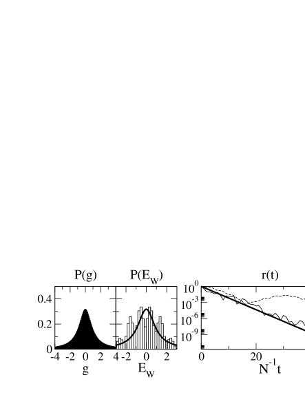
Figure 4: Same as Fig. 3 but for a Lorentzian distribution of the couplings ${g_{k}}$. In this case $r(t)$ decays exponentially. The histogram and the dashed line in $r(t)$ correspond to $N=20$, the straight thin line is a particular case for $N=100$ and the thick line is the average. We note that the convergence is slower than in the Gaussian case of Fig. 2, because realizations of ${g_{k}}$ are more likely to have one or two dominant couplings. Therefore, although the average shows a clear exponential decay, fluctuations are noticeable even for large $N$. Notice also that the logarithmic scale confirms the long time saturation of $r(t)$ at $\sim 2^{-N/2}$, Eq (7).

V Partial Reversal and Gaussian Echo

Let us now consider a Loschmidt echo – reversal of the sign of the Hamiltonian – carried out at a time $t_{R}$. In our model it can be implemented by appropriate “flipping” of the spins in the environment. We first note that the measured observable $\mu(t)$ signal can be readily related to the decoherence factor:

$$\mu(t) = Tr\rho_{\cal S}(t)\rho_{\cal S}(0)$$ (24)

$$= (a^{*}\langle 0|+b^{*}\langle 1|)\rho_{\cal S}(t)(a|0\rangle+b|1\rangle)$$

$$= |a|^{4}|+|b|^{4}+2|ab|^{2}Re~{}r(t)$$

For a complete Loschmidt echo, the sign of the the whole Hamiltonian would be reversed at $t=t_{R}$, so for $t>t_{R}$;

$$\mu(t)=|a|^{4}|+|b|^{4}+2|ab|^{2}Re~{}r(t_{R}-(t-t_{R}))\ .$$ (25)

Hence, the decoherence factor is now $r(2t_{R}-t)$, and the system will return to its initial state at $t=2t_{R}$.

We now suppose with Petitjean and Jacquod jacquod that only a part of the Hamiltonian is reversed (e.g., only some of the spins – spins in ${\cal E}^{\prime\prime}$ – get flipped). In our model, environments ${\cal E}^{\prime}$ and ${\cal E}^{\prime\prime}$ do not interact. Thus, the net decoherence factor is a product of the decoherence factors coming from each environment,

$$r(t)=r^{\prime}(t)r^{\prime\prime}(t),$$ (26)

with

$$r^{\prime}(t) \approx e^{iE_{N^{\prime}}t}\exp\left(-B_{N^{\prime}}^{2}t^{2}/2\right)$$ (27)

$$= e^{i\sum g_{k}^{\prime}t}\exp\left(-\sum(g_{k}^{\prime})^{2}t^{2}/2\right)$$

and

$$r^{\prime\prime}(t) \approx e^{i{E_{N^{\prime\prime}}(2t_{R}-t)}}\exp\left(-B_{N^{\prime\prime}}^{2}(2t_{R}-t)^{2}/2\right)$$ (28)

$$= e^{i\sum g_{k}^{\prime\prime}(2t_{R}-t)}\exp\left(-\sum(g_{k}^{\prime\prime})^{2}(2t_{R}-t)^{2}/2\right)\ .$$

Since the time reversal only applies to ${\cal E}^{\prime\prime}$,

$$\mu(t)=|a|^{4}|+|b|^{4}+2|ab|^{2}Re~{}r^{\prime}(t)r^{\prime\prime}(2t_{R}-t)\ .$$ (29)

At the instant $t=2t_{R}$ when the echo signal is usually acquired $r^{\prime}(2t_{R})=1$ and:

$$r(2t_{R}) = e^{i2E_{N^{\prime}}t_{R}}\exp\left(-\frac{B_{N^{\prime}}^{2}(2t_{R})^{2}}{2}\right)$$ (30)

$$= e^{i2\sum g_{k}^{\prime}t_{R}}\exp\left(-2\sum(g_{k}^{\prime})^{2}t_{R}^{2}\right)\ .$$

Thus, reversal is incomplete. The deficit in the signal exhibits a Gaussian dependence on the instant of reversal $t_{R}$. This is the effect of the on-going decoherence due to ${\cal E}^{\prime}$ – these spins in the environment that did not get reversed.

These equations exhibit the Gaussian time dependence (e.g., of the echo signal on the time of reversal $t_{R}$) for large values of $t_{R}$ (i.e., beyond the initial quadratic regime) as was found in some of the Loschmidt echo experiments carried out by Levstein and Pastawski horaciobook (see Fig. 5). Most importantly, the partial reversal provides an explanation of the surprising experimentally observed insensitivity of the Gaussian decay of polarization to the details of the pulse that initiates reversal: As noted in Ref. horaciosaturation , one might have expected that reversal pulse with larger amplitude will “turn back” evolution in a larger fraction of the environment, but this does not seem to happen. Rather, independence of the “backwards evolution” of the pulse inducing reversal indicates that always the same subset of the environment is turned back. It is therefore tempting to interpret their experimental results using the “two environment” theory we have outlined above. We believe that such interpretation is basically correct, but that a more careful discussion should take into account differences between the system investigated in Ref. horaciobook and our simple model.

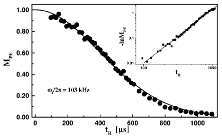
Figure 5: Attenuation of the polarization echoes in a single crystal of ferrocene as a function of reversal time $t_{R}$: The data correspond to an orientation where the two molecules per unit cell are magnetically equivalent. The solid line corresponds to a Gaussian fitting yielding a characteristic time $T=(400\pm 10)$ms as the single free parameter. The inset shows in effect $\ln(\mu(2t_{0})-\mu(\infty))$ vs $t_{0}$ in a log-log plot. The slope of the resulting line is $2.1\pm 0.08$, and is consistent with Eq. (30) (This illustration, Fig. 11 of Ref. horaciobook , is reproduced here by permission of the authors.)

This view of the above data seems especially appropriate since in ferrocene ($Fe(C_{5}H_{5})_{2}$, the molecule used in Ref. horaciosaturation ) there are (at least) two environments that are likely to respond differently to the attempted “Loschmidt reversal” of the dynamics. To point them out we need a bit more detailed description of the experiment. The ferrocene molecule (Fig. 6) consists of two rings, each with 5 hydrogen atoms attached to 5 carbon atoms. The Loschmidt echo experiment starts when a rare ${}^{13}C$ atom (that appears in a small fraction of all the molecules) is polarized by the external field that starts the experiment. This polarization is then transferred to its adjacent hydrogen. Once it is there, it can easily “diffuse” to the other hydrogens within the ring (or possibly within the molecule). This process is rapid; a brief ($\sim 100\mu s$) approximately Gaussian decay leads to an ondulating plateau. The hydrogen adjacent to the ${}^{13}C$ atom is about $20\%$ polarized at this instant (see Fig. 7).

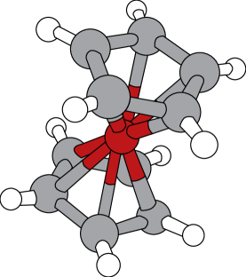
Figure 6: Schematic representation of a ferrocene ($Fe(C_{5}H_{5})_{2}$) molecule. The hydrogens (white, on the outside) are coupled to the carbon atoms (light grey) which form a pentagon ring. The two rings are joined in the middle by an iron atom (dark grey). They can rotate with respect to each other and with respect to the solid matrix in which ferrocene is imbedded, which suggests natural division into the immediate environment that can be effectively reversed and the more distant environment where the reversal is likely to fail.

Up to that point, the agreement between the numerical simulation of quantum evolution in a single ferrocene molecule and the experiment is remarkable, suggesting that the only environment explored by the injected polarization is the “immediate neighborhood”: hydrogens within the original $Fe(C_{5}H_{5})_{2}$. Indeed, the value of the numerical plateau ($\sim\frac{1}{5}$ of the original polarization) suggests that only the 5 hydrogens from the $C_{5}H_{5}$ “ring” that includes the rare ${}^{13}C$ atom participate early on.

By contrast with this initial interval, there is a marked discrepancy between the experiment and the single molecule simulations afterwards: Experimental data indicate leakage of the polarization from the molecule, with the signal decaying with time below the single molecule numerical prediction (see Fig. 7). As time goes on, both the measured and the simulated polarizations ondulate (indicating partial “revivals”, presumably because of the finite size of the ferrocene molecule horaciomeso ) but the experimental data also indicates persistent polarization leakage. Over the same time interval the simulation continues to hover just above $20\%$ of the original signal, and exhibits at best only much slower systematic decay.

Given the previous discussion, we have now reached the “eureka moment”: The immediate environment – hydrogens in the ferrocene (and, possibly, in only one of the $C_{5}H_{5}$ rings) are responsible for short term approximately Gaussian decay, and for the partial revivals, consistent with the behavior of such small quantum systems (as seen in Fig. 2). This is clearly a good candidate for our ${\cal E}^{\prime\prime}$ – the “reversible” part of the whole environment.

By contrast, once the signal leaks out to more distant ${\cal E}^{\prime}$ (which is responsible for the discrepancy between the single molecule simulations and the experimental data), “the cat is out of the bag”, and it (e.g., the polarization which has leaked out of the molecule) might be very difficult to recapture. This view is supported by what is known about the structure of solid ferrocene: Individual molecules (and, indeed, the two rings of the individual molecule) rotate on timescales short compared to these probed in the echo experiments. This dynamics will be much more difficult to reverse in the echo experiment.

The reversal will then result in the desired echo only on subsystems in which the atom has fixed neighbors (like the $C_{5}H_{5}$ ring), but is unlikely to succeed elsewhere. So, the environment of the ferrocene molecule (neighboring ferrocene molecules, and possibly even its other ring) constitute ${\cal E}^{\prime}$.

In closing this section we note that the timescale on which the echo decays is consistent with a Gaussian fit to the experimental data of the decay of the local polarization divided by the numerical simulation of the isolated molecule, see Fig. 7. The fit is consistent with an echo decay timescale of $4$ times the initial scale for decay of the local polarization, i.e. $\sim 400\mu s$ (see Fig. 5 for comparison). This is an ecouraging observation. Further, this scale would not be affected by a better reversal with the immediate environment ${\cal E}^{\prime\prime}$, consistent with the observed insensitivity of the echo to radiofrequency power horaciosaturation .

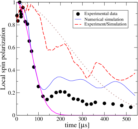
Figure 7: Evolution of the local spin polarization in a single crystal of ferrocene. The dots are the experimental data for a $0$ degree orientation of the crystal with respect to the external magnetic field. The thin solid line is the calculated evolution of the local polarization in a complete molecule where the rings rotate independently in a staggered configuration. The dashed line is the ratio between the simulation to the experimental data. The thick solid line is a Gaussian fit to the initial experimental data (up to $100\mu s$), and the thick dotted line is a fit to the ratio between experiment and simulation. The characteristic decay times of the fitted Gaussians are $90\mu s$ and $340\mu s$ respectively. This data is reproduced from Fig. 8 of Ref. horaciobook with permission from the authors.

VI Discussion

The model we have proposed is suggestive, but it is not yet conclusive: It offers only a rather simplified representation of the experiment. For instance, it is much more reasonable to say that the polarization first diffuses to the immediate “reversible” environment, and that the more remote environment decoheres all of this reversible ${\cal E}^{\prime\prime}$ (and not just the original system). Nevertheless, the split into two environments – our key assumption – explains the key features of the data in a way that naturally fits the physics of the system. However, it is useful to list at least some of the approximations we have made, and to consider their implications.

To begin with, interactions between the spins in Ref. horaciobook are dipolar, so the interaction Hamiltonian does not have the simple structure of the Ising Hamiltonian of Eq. (1). Moreover, spins of the real environment interact with each other. Furthermore, interaction and self-Hamiltonians of the spins do not commute in general.

Consequently, the straightforward manipulations that allowed us to derive Gaussian time dependence of the decoherence factor from first principles within a few lines cannot be directly carried out for more realistic models of the experiment. Nevertheless, the central ingredient needed to establish the Gaussian character of the echo does not seem to depend on these detailed assumptions. Rather, it is – in essence – the (approximately) Gaussian nature of the distribution of the eigenenergies of the total Hamiltonian, which then leads to the Gaussian time dependence of the decoherence factor. One can certainly believe that this very generic requirement is satisfied under conditions that are far more common than the specific assumptions of the simple decoherence model we have analyzed. Indeed, this broad applicability is the very essence of the central limit theorem we (and others HMH ) have invoked.

Even more convincing is the direct experimental evidence: Short time Gaussian dependence of the signal before reversal in the experiments involving ferrocene has been established horaciodifusion (see Fig. 5). This is in effect the decoherence factor – the characteristic function of the distribution of the relevant eigenenergies of the underlying Hamiltonian responsible for the evolution. And approximately Gaussian $r(t)$ implies (by the arguments involving Fourier transform) Gaussian eigenenergies.

Time evolution of the NMR polarization signal is in such settings often interpreted as diffusion Abragam ; DiffusionNMR . This makes intuitive sense in the experiments that lead to Fig. 5, as only rare nuclei of $C^{13}$ in a small fraction of ferrocene molecules are initially polarized, so the decay of the polarization signal is caused by the spreading of that polarization over an increasingly larger environment. However, this effective diffusion must obviously reflect a reversible dynamical process generated by an underlying Hamiltonian, as fundamentally diffusive evolution could never be reversed. This is reflected in the short time mesoscopic echoes observed in this “diffusive” process horaciomeso due to the small size of the first environment. To account for the diffusive character of the evolution the distribution of eigenenergies, $\eta(E)$ must be Gaussian in character. So, while specific assumptions we used in our simple model are not satisfied in the experimental setting, Gaussianity of the energy spectrum we were led to as a result of these assumptions may well turn out to be a fairly generic feature.

VII Summary and Conclusions

We have seen how – in the quantum setting of decoherence and Loschmidt echo – deterministic dynamics can lead to evolutions that have a distinctly stochastic Gaussian character. While our model is rather simple and clearly too idealized to directly address experimental situation of Refs. horaciobook ; horacioexponential ; horaciodifusion ; horaciosaturation , it also suggests that our main results – Gaussian decay of the decoherence factor and Gaussian echo – will appear whenever the energy spectrum of the excitation corresponding to the initial state of the system is approximately Gaussian. As we have noted earlier, there is ample evidence of this in the existing experiments involving ferrocene. Even more, we can reproduce the observed insensitivity to perturbations of the Gaussian echo decay. Qualitative – and even quantitative – comparisons between predictions of our model and the experimental data are promising.

We acknowledge useful discussions with Horacio M. Pastawski and Patricia R. Levstein. One of the authors (WHZ) acknowledges the Alexander von Humboldt Foundation Prize and the hospitality of the Center for Theoretical Physics of the University of Heidelberg, where part of this work was carried out.

References

- (1) M. Smoluchowski, Naturwissenschaften 6, 253 (1918).
- (2) W. H. Zurek, Phys. Rev. D 26, 1862 (1982).
- (3) W. H. Zurek, Phys. Rev. Lett. 90, 120404 (2003).
- (4) H. M. Pastawski, G. Usaj, and P. R. Levstein, in Contemporary Problems of Condensed Matter Physics, edited by S. J. Vlaev, L. M. Gaggero Sager, and V. V. Dvoeglazov (NOVA Scientific, New York, 2001).
- (5) G. Usaj, H. M. Pastawski, and P. R. Levstein, Mol. Phys. 95, 1229 (1998).
- (6) H. M. Pastawski, P. R. Levstein, G. Usaj, J. Raya, and J. Hirschinger, Physica A 283, 166 (2000).
- (7) P. R. Levstein, G. Usaj, and H. M. Pastawski, J. Chem. Phys. 108, 2718 (1998).
- (8) W. H. Zurek, Phys. Today 44, 36 (1991); J.-P. Paz and W. H. Zurek, in Coherent matter waves, Les Houches Session LXXII, R Kaiser, C Westbrook and F David eds., EDP Sciences (Springer Verlag, Berlin, 2001) 533-614; W. H. Zurek, Rev. Mod. Phys. 75, 715 (2003).
- (9) I. Zutic, J. Fabian, and S. Das Sarma, Rev. Mod. Phys. 76, 323 (2004); W. A. Coish, and D. Loss, Phys. Rev. B 70, 195340 (2004); L. Hartmann, J. Calsamiglia, W. Dür, and H.-J. Briegel, Phys. Rev. A 72, 052107 (2005); D. Rossini et al., quant-ph/0605051 and quant-ph/0611242 (2006).
- (10) W. H. Zurek. F. Cucchietti, and J.-P. Paz, quant-ph/0312207 (2003).
- (11) A. Kossakowski, Bull. Acad. Pol. Sci., Ser. Sci., Math. Astron. Phys. 21, 649 (1973); G. Lindblad, Commun. Math. Phys. 48, 119 (1976)
- (12) J. Preskill, Phys. Today 52 (6), 24 (1999); M. A. Nielsen and I. L. Chuang, Quantum computation and quantum information (Cambridge University Press, Cambridge, 2000).
- (13) J. Loschmidt, Sitzungsber. Kais. Akad. Wiss. Wien, Math. Naturwiss. Kl., II. Abt. 73, 128 (1876); ibid., III. Abt. 75, 267 (1877); ibid., IV. Abt. 76, 209 (1878).
- (14) T. S. Kuhn, Black Body Theory and Quantum Discontinuity, 1894-1912 (Oxford University Press, New York, 1978).
- (15) C. Petitjean and Ph. Jacquod, Phys. Rev. Lett. 97, 124103 (2006).
- (16) F. M. Cucchietti, D. A. R. Dalvit, J.-P. Paz, and W. H. Zurek, Phys. Rev. Lett. 91, 210403 (2003).
- (17) B. V. Gnedenko, The Theory of Probability, Fourth edition (Chelsea, New York,1968), see Chap. VIII.
- (18) G.Casati, B. V. Chirikov, I. Guarneri and F. M. Izrailev, Phys. Rev. E 48 R1613 (1993); Phys. Lett. A 223, 430 (1996).
- (19) L. Breiman, Probability, Classics in Applied Mathematics (SIAM, Philadelphia, 1992).
- (20) F. M. Cucchietti, W. H. Zurek and J.-P. Paz, Phys. Rev. A 72, 052113 (2005).
- (21) V. V. Dobrovitski, H. A. De Raedt, M. I. Katsnelson and B. N. Harmon, Phys. Rev. Lett. 90, 210401 (2003).
- (22) R. A. Jalabert and H. M. Pastawski, Phys. Rev. Lett. 86, 2490 (2001); P. Jacquod, P. G. Silvestrov, and C. W. J. Beenakker, Phys. Rev. E 64, 055203 (2001); F. M. Cucchietti, H. M. Pastawski, and R. A. Jalabert, cond-mat/0307752.
- (23) H. M. Pastawski, P. R. Levstein, and G. Usaj, Phys. Rev. Lett. 75, 4310 (1995).
- (24) E. Heller in Chaos and Quantum Physics, Proceedings of Session LII of the Les Houces Summer School, edited by A. Voros and M.J. Giannoni (North-Holland, Amsterdam, 1990).
- (25) A. Abragam, The principles of nuclear magnetism, Clarendon Press, Oxford (1978).
- (26) D. Braun, F. Haake, W. T. Strunz, Phys. Rev. Lett. 86, 2913 (2001).
- (27) M. Hartmann, G. Mahler, O. Hess, Lett. Math. Phys. 68, 103-112 (2004).
- (28) T. T. P. Cheung, Phys. Rev. B 23, 1404 (1981).
- (29) V. V. Dobrovitski and H. A. De Raedt, Phys. Rev. E 67, 056702 (2003); H. A. De Raedt and V. V. Dobrovitski, quant-ph/0301121.
- (30) J. Schliemann, A. V. Khaetskii and D. Loss, Phys. Rev. B 66, 245303 (2002).
- (31) V. K. B. Kota, Phys. Rep. 347, 223 (2001); V. V. Flambaum and F. M. Izrailev, Phys. Rev. E 61, 2539 (2000).