Determinable Solutions for One-dimensional Quantum Potentials: Scattering, Quasi-bound and Bound State Problems

Abstract

We derive analytic expressions of the recursive solutions to the Schrödinger’s equation by means of a cutoff potential technique for one-dimensional piecewise constant potentials. These solutions provide a method for accurately determining the transmission probabilities as well as the wave function in both classically accessible region and inaccessible region for any barrier potentials. It is also shown that the energy eigenvalues and the wave functions of bound states can be obtained for potential-well structures by exploiting this method. Calculational results of illustrative examples are shown in order to verify this method for treating barrier and potential-well problems.

I I. Introduction

Quantum mechanical tunneling and quantum well problems have attracted more interest, due to recent advances in the fabrication of semiconductor layers and the development of high-speed and novel devices Barnham and Vvedensky (2001). In order to better understand the physical properties of a device, it is important that one can accurately solve and analyze the one-dimensional potential problems. A number of methods for solving the Schrödinger’s equation and for locating the bound states and resonances generated by one-dimensional potentials have been developed over the past decades Brennan and Summers (1987); Ghatak et al. (1988); Jonsson and Eng (1990); Anemogiannis et al. (1999); Rakityansky (2004). Most of them are based on the so-called transfer-matrix approach. There are also some methods that are cumbersome to implement, for instance, the Monte Carlo method Singh (1986) and the finite element method (FEM) Nakamura et al. (1989).

In contrast to those numerical methods, a limited number of exact analytic solutions are available only for simple potential structures; analytic solutions are preferred due to its simple form and clear interpretation of the physics underlying the process. WKB method, as an approximate analytic approach, has been widely used but it is restricted to slowly varying potential profiles that are continuous. Improved methods such as the modified conventional WKB (MWKB)Love and Winkler (1977) and the modified Airy functions (MAF)Ghatak et al. (1992) still fail to provide perfect results.

TikochinskyTikochinsky (1977) has derived two nonlinear first-order equations replacing the second-order linear Schrödinger’s equation in a cutoff potential method for one-dimensional scattering amplitudes. In this paper we solve these nonlinear first-order equations analytically and obtain recursive solutions of the Schrödinger’s equation for multi-step barrier potentials. We intend to find a method providing a general analysis of the one-dimensional problem for both classically accessible region and inaccessible region. In fact, arbitrarily accurate solutions including the scattering amplitudes and the wave functions are obtainable with these recursive solutions for any potential profile by dividing it into many segments, since any continuous potential problem can be recovered as the segments become finer and finer.

Using the recursive solutions, we will also determine the wave functions of quasi-bound and bound states. We can solve a potential-well problem by evenly uplifting the potential function restricted on the potential-well region and its surroundings to construct a resonant barrier-potential that can readily be handled as a model potential. The resonant barrier-potential constitutes a quasi-bound-state problem, therefore each sharp tunneling resonance is locatable so that a quasi-bound-state eigenvalue can be determined which immediately leads to a bound-state eigenvalue being sought for the original potential well. Then, we can determine the eigenfunction belonging to the quasi-bound-state eigenvalue by means of the recursive solutions.

In Section II, we review the basic formalism for the one-dimensional problems that allows two nonlinear first-order equations to replace the linear second-order Schrödinger’s equation. In section III, we derive analytic expressions with recursive coefficients by solving the nonlinear equations for the transmission amplitudes, reflection amplitudes, and the wave functions for piecewise constant potentials. In section IV, a quasi-bound potential profile which characterizes a resonant tunneling is considered as the model potential of a potential well in order to treat bound-state problems. In section V and VI, we demonstrate the validity of the method by taking some examples, and discuss the calculational results.

II II. Basic Formalism

The one-dimensional Schrödinger equation for a particle with mass $m$ incident upon a potential energy $U(z)$ that asymptotically vanishes can be written as

$$\left({{d^{2}}\over{dx^{2}}}+k^{2}\right)\psi(x)=V(x)\psi(x)$$ (1)

where $x=z\sqrt{2m\epsilon/\hbar^{2}}$, $k^{2}=K/\epsilon$, and $V(x)=U(z)/\epsilon$ with a certain unit energy $\epsilon$ chosen for convenience. Here, $z$ is the position of the particle in the one-dimensional coordinate, $K$ is the energy of the particle, and $\hbar=h/2\pi$, $h$ being Planck’s constant. Thus, the coordinate $x$, the wave number $k$ and the potential $V(x)$ are all dimensionless. The dimensionless energy $E$ is defined by

$$E=k^{2}.$$ (2)

Now. we introduce a cutoff potential that was used in Refs. Tikochinsky, 1977; Goodvin and Shegelski, 2005a, b; Razavy, 2003. The cutoff potential is defined by

$$V_{c}(y,x)=V(x)\theta(x-y),$$ (3)

where $\theta(x-y)$ is the step function. If $V(x)$ is replaced by the cutoff potential, Eq. (1) has the formal solution:

$$\psi_{E}(y,x)=Ae^{ikx}+{{1}\over{2ik}}\int e^{ik|x-x^{\prime}|}V_{c}(y,x^{\prime})\psi_{E}(y,x^{\prime})dx^{\prime}.$$ (4)

Then, the cutoff reflection and cutoff transmission amplitudes for this problem can, respectively, be written as

$$R_{E}(y)={{1}\over{2ikA}}\int e^{ikx^{\prime}}V_{c}(y,x^{\prime})\psi_{E}(y,x^{\prime})dx^{\prime}$$ (5)

and

$$T_{E}(y)=1+{{1}\over{2ikA}}\int e^{-ikx^{\prime}}V_{c}(y,x^{\prime})\psi_{E}(y,x^{\prime})dx^{\prime}.$$ (6)

In Ref. Tikochinsky, 1977 it has been shown that the problem can be stated as two nonlinear first order equations given by

$${{dR_{E}(y)}\over{dy}}=-{{1}\over{2ik}}V(y)\left[e^{iky}+e^{-iky}R_{E}(y)\right]^{2}$$ (7)

and

$${{dT_{E}(y)}\over{dy}}=-{{e^{-iky}}\over{2ik}}V(y)\left[e^{iky}+e^{-iky}R_{E}(y)\right]T_{E}(y),$$ (8)

with the boundary conditions, $R_{E}(\infty)=0$ and $T_{E}(\infty)=1$. The Schrödinger’s equation, which is a second-order differential equation, has been disassembled through the cutoff-potential manipulation into two first-order equations, Eqs. (7) and (8). Integration of Eq. (8) immediately leads to

$$T_{E}(x)=\exp\left(\int_{x}^{\infty}{{e^{-iky}}\over{2ik}}V(y)\left[e^{iky}+e^{-iky}R_{E}(y)\right]dy\right).$$ (9)

The reflection amplitude $R_{E}$ and the transmission amplitude $T_{E}$ for the potential $V(x)$ are $R_{E}=R_{E}(-\infty)$ and $T_{E}=T_{E}(-\infty)$ in terms of which the reflection and transmission probabilities are, respectively, given as

$$P_{R}=\left|R_{E}\right|^{2}$$ (10)

$$P_{T}={{k_{f}}\over{k}}\left|T_{E}\right|^{2},$$ (11)

where $k_{f}=\sqrt{E-V(\infty)}$.

III III. The Piecewise-constant Potential Problem

We want to find analytic expressions of the transmission amplitude, reflection amplitude and the wave function for a multi-step potential profile which contains $n$ layers of constant potential in the zero-potential environment, as shown in Fig. 1. Let us solve Eq. (7) for $R_{E}(x)$ in $j$th step region ($b_{j-1}<x<b_{j}$) for $V(x)=V_{j}\neq 0$, where $V_{j}$ is constant for $j=1,\cdots,n$. By defining

$$Q_{E}(x)=R_{E}(x)e^{-2ikx}+1-{{2k^{2}}\over{V_{j}}}$$ (12)

Eq. (7) can be rewritten as

$${{dQ_{E}(x)}\over{dx}}=i{{V_{j}}\over{2k}}\left[\left(Q_{E}(x)\right)^{2}+\left({{4k^{2}}\over{V_{j}^{2}}}(V_{j}-k^{2})\right)\right]$$ (13)

to which the solution is

$$Q_{E}(x)=i2k{{p_{j}}\over{V_{j}}}\left({{1+A_{j}e^{-2p_{j}x}}\over{1-A_{j}e^{-2p_{j}x}}}\right)$$ (14)

with a constant $A_{j}$ to be determined by a boundary condition. Here, $p_{j}$ is defined by

$$p_{j}=\left\{\begin{array}[]{ll}\sqrt{V_{j}-k^{2}}&\mbox{for $V_{j}>k^{2}$},\\ i\sqrt{k^{2}-V_{j}}&\mbox{for $V_{j}<k^{2}$}.\end{array}\right.$$ (17)

Then, we obtain the cutoff reflection amplitude in the $j$th step region:

$$R_{E}(x)=\left[{{2k^{2}}\over{V_{j}}}-1+i2k{{p_{j}}\over{V_{j}}}\left({{1+A_{j}e^{-2p_{j}x}}\over{1-A_{j}e^{-2p_{j}x}}}\right)\right]e^{2ikx}.$$ (18)

On the other hand, the solution of Eq. (7) for $V_{j}=0$ in the $j$th step region is

$$R_{E}(x)=C_{j}$$ (19)

which can be determined by the continuity condition of $R_{E}(x)$ at the boundary $x=b_{j}$.

Figure 1:

A multi-step potential profile consisting of $n$ steps in the zero-potential environment.

If $V_{j+1}=0$, $R_{E}(x)=C_{j+1}$ in the region $b_{j}<x<b_{j+1}$ and the continuity of $R_{E}(x)$ at the boundary $x=b_{j}$ leads to

$$A_{j}=\left({{V_{j}(C_{j+1}e^{-2ikb_{j}}+1)-2k^{2}-i2kp_{j}}\over{V_{j}(C_{j+1}e^{-2ikb_{j}}+1)-2k^{2}+i2kp_{j}}}\right)e^{2p_{j}b_{j}}.$$ (20)

But, if $V_{j+1}\neq 0$, the boundary condition gives

$$A_{j}=\left({{D_{j}-V_{j+1}p_{j}+ik(V_{j+1}-V_{j})}\over{D_{j}+V_{j+1}p_{j}+ik(V_{j+1}-V_{j})}}\right)e^{2p_{j}b_{j}},$$ (21)

where

$$D_{j}=V_{j}\,p_{j+1}\left({{1+A_{j+1}e^{-2p_{j+1}b_{j}}}\over{1-A_{j+1}e^{-2p_{j+1}b_{j}}}}\right).$$ (22)

Let us take the index $j=n+1$ for the region $x>b_{n}$. Since $V_{n+1}=0$ and $p_{n+1}=ik$, we obtain $A_{n+1}=0$ from (20). $A_{j}$ is related to $A_{j+1}$ through Eq. (21) if $V_{j+1}\neq 0$, while it is related to the constant reflection amplitude $C_{j+1}$ through Eq. (20) if $V_{j+1}=0$. Therefore, all $A_{j}$’s for $j=1,\cdots,n$ can be determined recursively from the starting value $A_{n+1}=0$.

The cutoff transmission amplitude $T_{E}(x)$ can be obtained in the $j$th step region ($b_{j-1}<x<b_{j}$) from Eq. (9) by the help of (18).

$$T_{E}(x) = T_{E}(b_{j})\exp\left[(p_{j}-ik)(b_{j}-x)\right]$$ (23)

$$\times\left({{1-A_{j}e^{-2p_{j}b_{j}}}\over{1-A_{j}e^{-2p_{j}x}}}\right)$$

where

$$T_{E}(b_{j}) = \prod_{l=j+1}^{n}\exp\left[(p_{l}-ik)(b_{l}-b_{l-1})\right]$$ (24)

$$\times\left({{1-A_{l}e^{-2p_{l}b_{l}}}\over{1-A_{l}e^{-2p_{l}b_{l-1}}}}\right).$$

Therefore, the analytic expression of the transmission amplitude is

$$T_{E} = T_{E}(-\infty)=\prod_{l=1}^{n}\exp\left[(p_{l}-ik)(b_{l}-b_{l-1})\right]$$ (25)

$$\times\left({{1-A_{l}e^{-2p_{l}b_{l}}}\over{1-A_{l}e^{-2p_{l}b_{l-1}}}}\right).$$

From Eqs. (4) and (5)

$$\psi_{E}(y,y)=A\left[e^{iky}+e^{-iky}R_{E}(y)\right]$$ (26)

and by differentiating Eq. (4) in the region $y<x$ one has the relation

$${{\partial\psi_{E}(y,x)}\over{\partial y}} = -{{e^{-iky}V(y)}\over{2ik}}\psi_{E}(y,y)e^{ikx}$$

$$+ {{1}\over{2ik}}\int e^{ik|x-x^{\prime}|}V_{c}(y,x^{\prime}){{\partial\psi_{E}(y,x^{\prime})}\over{\partial y}}dx^{\prime}.$$

Eq. (4) and Eq. (III) are both the solution of Eq. (1) with the cutoff potential $V_{c}(y,x)$ but have different amplitudes. Their amplitudes differ by a factor $-e^{-iky}V(y)\psi_{E}(y,y)/2ikA$, thus in the region $y<x$

$${{\partial\psi_{E}(y,x)}\over{\partial y}}=-{{e^{-iky}V(y)}\over{2ik}}\left[e^{iky}+e^{-iky}R_{E}(y)\right]\psi_{E}(y,x).$$ (28)

Integration of Eq. (28) in the region $y<x$ leads to

$${{\psi_{E}(x,x)}\over{\psi_{E}(x)}}={{\psi_{E}(x,x)}\over{\psi_{E}(-\infty,x)}}$$

$$= \exp\left(-\int_{-\infty}^{x}{{e^{-iky}}\over{2ik}}V(y)\left[e^{iky}+e^{-iky}R_{E}(y)\right]dy\right)$$

which can be rewritten, with the aid of Eq. (9), as

$$\psi_{E}(x)=A{{T_{E}}\over{T_{E}(x)}}\left[e^{ikx}+e^{-ikx}R_{E}(x)\right].$$ (30)

One can imagine the insertion of an infinitesimally thin virtual layer of zero potential at $x$, and consider the wave function $\psi_{E}(x)$ to be the superposition of the forward traveling wave $e^{ikx}$ and the backward traveling wave $R_{E}(x)~{}e^{-ikx}$ reflected upon the potential on the right side of the virtual layer, multiplied by the factor $AT_{E}/T_{E}(x)$ which is fathomable to be the correct amplitude for the superposed wave function at $x$.

Substituting (23) and (25) into Eq. (30), we write the wave function for the energy $E$ in the $j$th layer ($b_{j-1}<x<b_{j}$) as

$$\psi_{jE}(x) = A\prod_{l=1}^{j}\exp\left[(p_{l}-ik)(b_{l}-b_{l-1})\right]\left({{1-A_{l}e^{-2p_{l}b_{l}}}\over{1-A_{l}e^{-2p_{l}b_{l-1}}}}\right)$$ (31)

$$\times \exp\left[(p_{j}-ik)(x-b_{j})\right]\left({{1-A_{j}e^{-2p_{j}x}}\over{1-A_{j}e^{-2p_{j}b_{j}}}}\right)\left[e^{ikx}+e^{-ikx}R_{E}(x)\right]$$

$$= A\prod_{l=1}^{j}\exp\left[(p_{l}-ik)(b_{l}-b_{l-1})\right]\left({{1-A_{l}e^{-2p_{l}b_{l}}}\over{1-A_{l}e^{-2p_{l}b_{l-1}}}}\right)$$

$$\times {{2ik\exp\left[(ik-p_{j})b_{j}\right]}\over{V_{j}\left[1-A_{j}\exp\left(-2p_{j}b_{j}\right)\right]}}\left[\left(-ik+p_{j}\right)e^{p_{j}x}+A_{j}\left(ik+p_{j}\right)e^{-p_{j}x}\right].$$

Eq. (31) is an analytic expression for the recursive solution of the Schrödinger equation. It is simple and fast to calculate $A_{j}$’s for any multi-step potential. Also, any continuous potential problem may be considered to be a multi-step potential problem by dividing the non-zero potential region into a lot of small segments such that the potential in each segment can be approximated to a specific value, for instance, the average value, of the continuous potential within the segment. Thus, the analytic expression of the wave function given by Eq. (31) can be used for obtaining an arbitrarily accurate solution for any one-dimensional potential.

In passing, let us check that Eq. (31) is consistent with the traveling plane waves which are expected in the regions $x<b_{0}$ and $x>b_{n}$, where $V(x)=0$. Without loss of generality, one may take the first step region ($b_{0}<x<b_{1}$) such that $V_{1}=0$. Then, the wave function in the region $x<b_{1}$ becomes

$$\psi_{1E}(x)= \lim_{V_{1}\rightarrow 0}A(e^{ikx}+e^{-ikx}R_{E}(x))$$

$$\times\exp[(p_{1}-ik)(x-b_{0})]\frac{1-A_{1}e^{-2p_{1}x}}{1-A_{1}e^{-2p_{1}b_{0}}}$$

$$= A\left[e^{ikx}+R_{E}~{}e^{-ikx}\right],$$ (32)

since $A_{1}=-(V_{1}/4k^{2})R_{E}$ from Eq. (18) for the limit $V_{1}\rightarrow 0$. On the other hand, if we take the last step region $b_{n-1}<x<b_{n}$ such that $V(x)=V_{n}=0$, the wavefunction in the region $x>b_{n-1}$ becomes

$$\psi_{nE}(x)=AT_{E}~{}e^{ikx},$$ (33)

since $R_{E}(x)=0$ and $A_{n}=-(V_{n}/4k^{2})R_{E}(x)$ from Eqs. (18) and (25) in the limit $V_{n}\rightarrow 0$. Eqs. (III) and (33) show that Eq. (31) is consistent as the solution of Eq. (1) in the zero-potential region.

IV IV. Quasi-bound States

We consider a resonant barrier structure that consists of $n$ layers of piecewise constant potential. Resonances are supposed to occur at energies less than both $V_{1}$ and $V_{n}$ which are potential values of the end steps so that quasi-bound states are involved. The wave function $\psi_{jE}(x)$ in $j$th layer for this structure can be obtained with the calculated $A_{j}$’s which are dependent on $E$. $A_{n}$, in the last layer, can be evaluated from (20) with cutoff reflection amplitude $C_{n+1}=0$. Inserting the evaluated $A_{n}$ into (31), we find in the last layer for $E<V_{n}$

$$\psi_{nE}(x) \propto (-ik+p_{n})e^{p_{n}x}$$

$$+ {{V_{n}-2k^{2}-2ikp_{n}}\over{V_{n}-2k^{2}+2ikp_{n}}}(ik+p_{n})e^{p_{n}(2b_{n}-x)},$$

where the first term exponentially increases with increasing $x$, while the second term exponentially decreases. One can see that if $p_{n}(b_{n}-b_{n-1})$ is large enough, the first term is negligible in magnitude compared with the second term, so the wave function exponentially damps with increasing $x$ in the region $b_{n-1}<x<b_{n}$.

Now, let us consider the wave function in the first layer which is given from (31) by

$$\psi_{1E}(x) = A{{2ike^{ikb_{0}}}\over{V_{1}(e^{p_{1}b_{0}}-A_{1}e^{-p_{1}b_{0}})}}$$

$$\left[(-ik+p_{1})e^{p_{1}x}+(ik+p_{1})A_{1}e^{-p_{1}x}\right],$$

where $A_{1}$ is obtained through the step potential profile of the resonant barrier structure. The wave function given by Eq. (IV) exponentially increases with increasing $x$ when $|A_{1}|=0$; $A_{1}$ vanishes at the energies of quasi-bound states. $|A_{1}|=0$ may be used as the quantization condition for the energy levels of a particle confined in a potential well. In the practical calculations, transmission resonances occur at the energies where $|A_{1}|$ takes a minimum value in a sudden dip, if $b_{1}-b_{0}$ and $b_{n}-b_{n-1}$ are large enough. Such resonances indicate quasi-bound states.

Now, a potential well can be treated by uplifting the potential function restricted on the region of the well and its surroundings to form a resonant barrier structure that can be handled in our approach. This resonant structure is used as a model potential of the potential well under consideration. Then, each resonance occurred in this model-potential problem corresponds to an energy eigenvalue for the potential well, and the real part or the imaginary part of the quasi-bound-state function obtained for a resonant energy is the eigenfunction of the bound state belonging to the corresponding eigenvalue for the potential well within a normalization constant.

V V. Some Examples

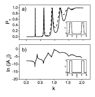
Figure 2:

(a) Transmission probabilities of double-barrier potentials: the solid line and the dashed line are for the square and the gaussian double-barrier potential, respectively. Their potential profiles are shown in the inset graph. (b) The curve of $\ln{(|A_{1}|)}$ for the double square-barrier potential. Its profile is in the inset graph. Each dip of the $\ln(|A_{1}|)$ curve below the barrier exactly agrees with the resonant peak of transmission probability shown in (a).

In order to demonstrate the validity of our method, we consider quantum barriers and quantum well potentials. Here, we examine the derived recursive expressions of the transmission amplitude and the state wave-function given by Eqs. (25) and (31), respectively, by calculating $A_{j}$’s for several potentials.

First, we consider rectangular and gaussian double-barrier potentials which are shown in the inset of Fig. 2(a). Here, the unit energy $\epsilon$ is chosen to be the maximum potential energy of the barrier. Since the rectangular double barrier structure consists of three layers of constant potential, the analytic expression of the recursive solution $\psi_{jE}(x)$ for this structure can be obtained with calculated $A_{j}$’s which are dependent on $E$. One can determine $A_{3}$ from Eq. (20) with the cutoff reflection amplitude $C_{4}=R_{E}(x)=0$ in the region $x>b_{3}$, and determine $C_{2}$ for the step region of $j=2$ where $V_{2}=0$ by evaluating $R_{E}(x)$ at $x=b_{2}$ in the step region of $j=3$ through Eq. (18). Then, $A_{1}$ can be also obtained through Eq. (20) using the value of $C_{2}$. Fig. 2(b) shows the curve of $\ln(|A_{1}|)$ for the rectangular double barrier structure. Each dip of the curve coincides with a transmission resonance for the energy below the barrier ($k<1$) as shown in Fig. 2. Such a sharp dip of $A_{1}$ indicates that an exponentially increasing term of the wave function is dominant in the first barrier region due to a negligibly small $|A_{1}|$ as was considered below Eq. (IV), so that the transmission probability becomes large in the narrow energy region. The resultant transmission probabilities for the two barrier profiles have similar resonance patterns as shown in Fig. 2(a). We have confirmed that the solid line for the rectangular double barrier perfectly agrees with the result obtained by the traditional method for solving the Schrödinger’s equation for step potential problems with boundary conditions imposed.

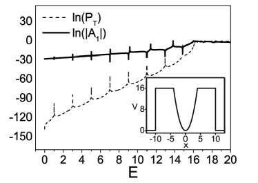
Figure 3:

Resonances for a model potential of harmonic oscillator given by Eq. (39). Each sharp dips on the solid line of the curve $\ln{(|A_{1}|)}$ exactly agrees with a resonant peak on the dashed line of the curve $\ln{(P_{T})}$.

Next, we consider a potential model by which one can obtain eigenvalues and eigenfunctions for a harmonic oscillator. We take the unit energy to be $\epsilon=\hbar\omega/2$, where $\omega$ is the characteristic angular frequency of the harmonic oscillator. Then, the dimensionless potential in Eq. (1) is $V_{ho}=x^{2}$ for the harmonic oscillator. In order to apply our method to the harmonic oscillator in an energy range $0<E<16$, we employ a model potential:

$$V_{HO}(x)=\left\{\begin{array}[]{ll}x^{2}&\mbox{for $|x|<4$}\\ 16&\mbox{for $4<|x|<10$}\\ 0&\mbox{for $|x|>10$},\end{array}\right.$$ (39)

as shown in the inset of Fig. 3. This model has a double barrier structure and represents a quasi-bound problem in which the transmission of a particle through the model potential reaches its peak when the energy is resonant with one of the energy levels of the quasi-bound states in the region between the two potential barriers. The potential in Eq. (39) is expected to involve low quasi-bound-state energies that approximately equal the bound state energies of the harmonic oscillator, respectively. Each sharp dip of $\ln(|A_{1}|)$ suppresses the term exponentially decreasing with increasing $x$ in the wave function in Eq. (31) allowing the exponentially increasing term to be dominant in the first barrier, and thus occurs at the same energy as a resonance peak which locates a quasi-bound state, as shown in Fig. 3. Energies of the quasi-bound states have been determined very accurately to fit in the exact eigenvalues of the harmonic oscillator $E_{n}=2n+1$ with $n=0,1,2,\cdots$ for the low lying states. However, there are very small errors for the upper levels, for instance, $n=5,6,7$, because the model potential in Eq. (39) is different from the potential of the harmonic oscillator for the region $|x|>4$.

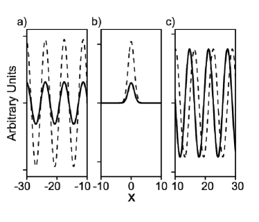
Figure 4:

The wave function of the lowest quasi-bound state ($E=1.0$) for the potential given by Eq. (39) for three regions with different units. The solid line and dashed line are the real and imaginary parts of the wave function, respectively.

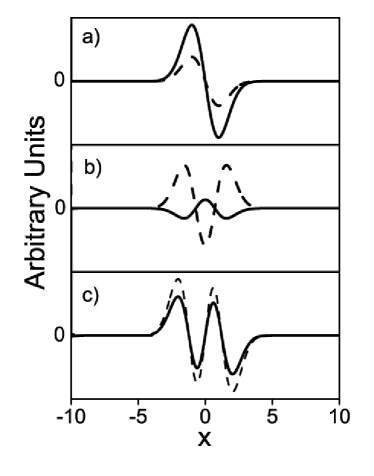
Figure 5:

The wave functions of three quasi-bound states of energies, (a) $E=3.0$, (b) $E=5.0$ and (c) $E=7.0$, for the potential given by Eq. (39). The solid lines and dashed lines are the real and imaginary parts of the wave functions, respectively.

Once a quasi-bound-state eigenvalue is determined, the wave function of the state can be obtained from Eq. (31). The lowest quasi-bound state for the model potential in Eq. (39) corresponds to the ground state for the harmonic oscillator. The wave function of the state is separately shown in Fig. 4 for the regions, $-30<x<-10$, $-10<x<10$, and $10<x<30$ with different units. The solid line and dashed line are, respectively, the real part and the imaginary part of the wave function. The forward and reflected plane waves are superposed in the region $x<-10$, and only the transmitted forward plane-wave propagates in the region $x>10$. One can see in Fig. 4(b) that the wave function exponentially increases with increasing $x$ in the first barrier region at the resonance energy but exponentially decreases in the second barrier region which is sufficiently wide as explained earlier, forming the lowest quasi-bound-state wave function in the binding potential region between the two barriers. Wave functions of the next three quasi-bound states for the same model potential that correspond to the three lowest excited states in the harmonic oscillator problem are also shown in Fig. 5. Either the real part or the imaginary part of a quasi-bound-state wave function can be taken as the wave function of the corresponding bound state for the harmonic oscillator.

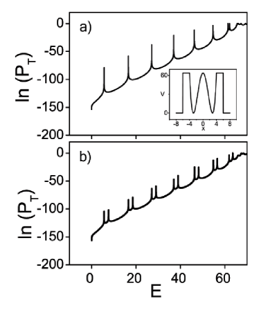
Figure 6:

Logarithmic transmission probabilities for double-well model potentials given by (a) Eq. (46) and (b) Eq. (47). Each peak represents transmission resonance.

For our final example, we consider a symmetric double-well potential given by

$$V_{dw}(x)=\left\{\begin{array}[]{ll}x^{2}(x^{2}-16)&\mbox{for $|x|<4$},\\ 0&\mbox{for $|x|>4$}.\end{array}\right.$$ (42)

For treating this problem with our methods, we take a model potential of $V_{dw}$ by uplifting the potential function on the region $|x|<6$ by $64$:

$$V_{DW}(x)=\left\{\begin{array}[]{ll}x^{2}(x^{2}-16)+64&\mbox{for $|x|<4$},\\ 64&\mbox{for $4<|x|<6$},\\ 0&\mbox{for $|x|>6$},\end{array}\right.$$ (46)

which is shown in the inset of Fig. 6(a). The local maximum of the model potential located at $x=0$ is $64$, and the two local minima are located at $x=2\sqrt{2}$. The calculated curve for $\ln{P_{T}}$ is plotted in Fig. 6(a). As is well-known, each peak comprises a pair of states, an even state and an odd state, whose energies are the very same especially for a peak of lower energy. But they are not perfectly degenerate, since a particle in one potential well can tunnel into the other well through the middle barrier which is finite. The energy difference of two states comprised in a peak increases with increasing energy, and thus the seventh pair of states which are just below the barrier appears to be separated.

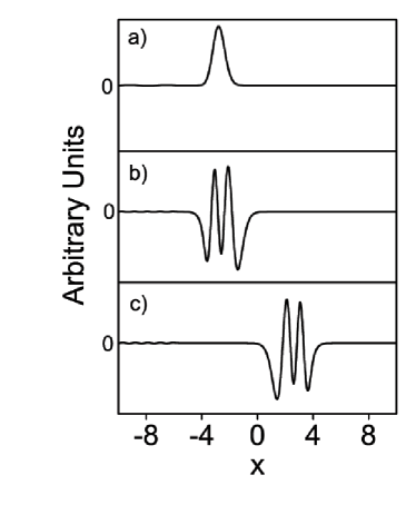
Figure 7:

The wave functions of three bound states for the double well potential, $V(x)=x^{2}(x^{2}-16)+\tanh x$; (a) the ground state, (b) the eighth excited state, and (c) the ninth excited state. These wave functions have been obtained by using the model potential given by Eq. (47) as explained in the text.

In order to confirm that two states are comprised in a peak, we add a small asymmetric potential function to the potential in Eq. (46):

$$V^{\prime}_{DW}(x)=V_{DW}(x)+V^{\prime}(x)=V_{DW}(x)+\tanh x+1.$$ (47)

Using this potential, we obtain a curve of $\ln|P_{T}|$ in which there are seven pairs of quasi-bound states as shown in Fig. 6(b). Each pair is split into two peaks due to the perturbing potential $V^{\prime}(x)$ from a peak containing two states for the double-well potential $V_{DW}$ shown in Fig. 6(a). The lower state and higher state in each pair are expected to be confined in the left well and right well, respectively.

In order to find bound-state wave functions for the double well potential given as $V(x)=x^{2}(x^{2}-16)+\tanh x$, one may take either the real parts or imaginary parts of quasi-bound-state wave functions determined from Eq. (31) for an appropriate model potential such as Eq. (47). The real parts (or imaginary parts) can be considered as the bound-state eigenfunctions within a normalization constant. Real parts of the wave function of the lowest ($n=0$), the ninth ($n=8$), and the tenth ($n=9$) quasi-bound states, which are taken to be the wave functions of corresponding bound states, are plotted in Fig. 7(a), (b) and (c), respectively. Fig. 7 shows that the particle which occupies the lowest state or the ninth state stays in the left potential well, while the particle occupying the tenth state stays in the right potential well, as expected.

VI VI. Discussions and Conclusion

Analytically solving two nonlinear first-order differential equations equivalent to the Schrödinger’s equation, we have obtained the recursive solutions of the cutoff reflection amplitude $R_{E}(x)$, the cutoff transmission amplitude $T_{E}(x)$ and the state wave function $\psi_{E}(x)$ for a multi-step potential. One can use the recursive solutions in Eqs. (25) and (31) for any piecewise constant potential to obtain transmission amplitudes and eigenfunctions, respectively. If an approximate multi-step potential consisting of sufficiently many layers is substituted for a smooth potential profile, calculations with the recursive solutions are accurate and fast.

For treating a potential well, we take a model potential with two side barriers that contains a partial profile identical to the profile of the potential well in the region between the side barriers. In the model potential problem, resonance occurs at the energy of a quasi-bound state, so the energies can be determined by locating the transmission resonances. Once a quasi-bound-state energy is known, the eigenfunction for the energy can also be determined. However, the real part and the imaginary part of the wave function of a quasi-bound state exponentially increases at a same rate in the first barrier and exponentially decrease in the last barrier as explained earlier, and are the same within a factor $\tan\phi$ in the region between two side barriers, $\phi$ being a phase angle. Therefore, either the real or the imaginary part can be taken for the wave function of the corresponding bound state with a normalization constant.

We have considered several examples to demonstrate the validity of our method with the recursive solutions. First, we have calculated the transmission probabilities of a particle incident upon a rectangular and a gaussian double-barrier potential which show typical features of resonant tunneling in Fig. 2(a). The rectangular double barrier simply consists of three layers, the left barrier being the first potential step, and the feature of resonant tunneling can be explained by the calculational results of $A_{1}$ in which information of the barrier structure is included. If $A_{1}=0$ for an energy lower than the barriers, the wave function does not contain exponentially decreasing term with increasing $x$ in the first barrier region so that it exponentially increases in the region, and thus the transmission probability reaches maximum at the energy. Practically, the sharp dips of the $\ln|A_{1}|$ curve in Fig. 2(b) represent the resonances associated with quasi-bound states in the rectangular well between the barriers.

The harmonic oscillator problem can be dealt with by solving a quasi-bound-state problem with the model potential given by Eq. (39). The calculational results for $\ln|A_{1}|$ and $\ln P_{T}$ are shown in Fig. 3, so the quasi-bound-state energies which may be regarded as the energy eigenvalues of the harmonic oscillator can readily be determined by locating the resonance peaks of $\ln P_{T}$ or the sharp dips of $\ln|A_{1}|$. The resultant peaks perfectly agree with the exact eigenvalues for low energy states, but deviate a little from the exact values for high energy states; $E_{0}=1.000$, $E_{1}=3.000$, $E_{2}=5.000$, $E_{3}=6.9999$ $E_{4}=8.999$, $E_{5}=10.994$, $E_{6}=12.970$, and $E_{7}=14.857$. Since the deviation originates from the approximated model potential which does not agree with the harmonic-oscillator potential on the high potential region $|x|>4$, one may get more accurate eigenvalues for higher states by using a larger model potential which coincides with the harmonic-oscillator potential in a wider region.

We have applied our method to a symmetric double-well potential given by Eq. (42), using Eq. (46) as its model potential. It is well-known that an even state and an odd state are folded together belonging closely to an eigenvalue if they are deeply bound in a symmetric double well whose middle barrier is strong enough so that the wave functions nearly vanish in the barrier region. The even state and odd state belonging to the same eigenvalue can be combined to constitute two bound states that are localized in the left well and right well with the same eigenvalue, respectively. Thus, one may consider each resonance peak to correspond to a pair of states confined in one and the other well, as well as a pair of even and odd states. When an asymmetric perturbing potential is added to the double-well potential, each resonance peak has been split into two peaks, as shown in Fig. 6(b). Since the potential is not symmetric due to the perturbation, even and odd states can not be sustained. Therefore, each resonance peak in Fig. 6(b) represents a state confined in one of the two wells. As expected, Fig. 7 shows that among the two states separated from each other due to the perturbation, the lower energy state is confined in the left well which is a little deeper than the right well, while the higher energy state is confined in the right-well region. The ninth (n=8) and tenth (n=9) states are the fifth states in the left well and the right well, respectively, so the numbers of nodes in their wave functions are identically four as in Fig 7 (b) and (c).

Here, more accurate determination of quasi-bound-state energies is required to obtain eigenfunctions of the lower quasi-bound-state confined in the right well, because the resonance is sharper for the particle tunneling into a deeper quasi-bound state or a state confined in the right well through the stronger barrier or two barriers (the first barrier and the middle barrier); for instance, the determined eigenvalues $E_{0}=5.601849104$, $E_{1}=7.58342367856952$, $E_{8}=46.290706$ and $E_{9}=48.1538536$ should be used in obtaining the wave functions, where $E_{1}$ is required to be the most accurate. Here, each bound-state energy for $V(x)=x^{2}(x^{2}-16)+\tanh x$ is the corresponding quasi-bound-state energy for $V^{\prime}_{DW}$ minus 65. Unlike the model potential of the harmonic oscillator, no approximation is involved in the calculation with the model potential of this double well potential.

Although here we have presented results for double barriers, a harmonic oscillator, and double-well potentials, the analysis can easily be applied for accurate calculations to general potential barrier and quantum well structures. The analysis could be extended to the one-dimensional problem of a particle that has a coordinate-dependent mass, by imposing the boundary conditions on the step potential structure. In addition, the three-dimensional Schrödinger equation for a spherically symmetric potential can also be solved using the present method because such a three-dimensional problem can be reduced to a one-dimensional problem.

In conclusion, we have described a method for solving the one-dimensional Schrödinger equation by means of the analytic expressions of recursive solutions derived for piecewise-constant potentials. The recursive solutions provide a general analysis of one-dimensional scattering, quasi-bound and bound state problems. We have demonstrated the validity of the method by taking some examples to show consistent and predictable calculational results. The calculations with the recursive solutions were rapid and accurate even for smoothly varying potentials.

VI.1