Controlled Creation of Spatial Superposition States for Single Atoms

Abstract

We present a method for the controlled and robust generation of spatial superposition states of single atoms in micro-traps. Using a counter-intuitive positioning sequence for the individual potentials and appropriately chosen trapping frequencies, we show that it is possible to selectively create two different orthogonal superposition states, which can in turn be used for quantum information purposes.

During recent years trapping and controlling small numbers of neutral atoms has emerged as one of the most active and productive frontier areas in research Haensel:01 ; Bergamini:04 ; Chuu:05 ; Shevchenko:06 . The interest in single atom systems is driven not only by the desire to perform experiments that answer longstanding and fundamental quantum mechanics questions Eschner:01 ; Beugnon:06 , but also by the desire to implement concepts of quantum information using neutral atoms Brennen:99 ; Jaksch:99 ; Jaksch:00 . Advances in the technology of optical lattices and micro-traps have recently allowed for substantial progress in this area Birkl:01 ; Rauschenbeutel:05 ; Yavuz:06 ; Sortais:06 and various concepts have been developed to prepare and process the states of single atoms in a controlled way. While techniques for controlling and preparing the internal states of atoms using appropriate electromagnetic fields are well developed, only few concepts exist for achieving the same control over the spatial part of a wavefunction Zhang:06 ; Eckert:04 ; Eckert:06 .

Three fundamental requirements for controlling the spatial part of a wavefunction are preparation, storage and transport. Optical and magnetic micro-potentials have proven to be robust tools for atom storage and techniques for moving particles between different potential sites using dedicated waveguides or sophisticated tunneling schemes have been suggested Arlt:01 ; Brugger:05 ; Mompart:03 . While waveguides are usually highly static, the tunneling interaction can be tuned by actively changing the distance between or the potential heights of neighboring traps. Both of these possibilities have recently been explored by Eckert et al. Eckert:04 ; Eckert:06 and Greentree et al. Greentree:04 . These works considered three modes in three separated potentials and suggested the use of a STIRAP-like process to achieve a robust transfer of an atom from one trap to another with high fidelity. In the area of three-level optics, the STIRAP process refers to the technique whereby a counter-intuitive application of laser pulses leads to a transition of an electron between the ground states in a $\Lambda$-system Bergmann:98 ; Vitanov:01 . In the atom trap scenario the energy levels are replaced by spatially separated trap ground states and the laser interaction is replaced by the coherent tunneling interaction. Eckert et al. also showed analogues for coherent population trapping and electromagnetically induced transparency Eckert:04 . They termed this new area three-level atom optics.

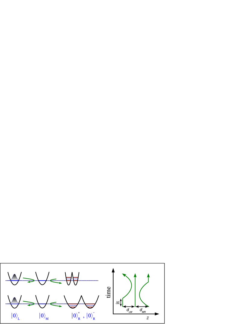
Figure 1: Left: The three atom traps are arranged in a linear fashion. The trap on the left and the trap in the middle are harmonic potentials and the double well trap on the right is made piecewise out of two harmonic traps. The trapping frequencies are arranged in such a manner that either the symmetric state (upper schematic) or the anti-symmetric state (lower schematic) of the double well is in resonance with the ground states of the other traps. The asymptotic ground states in the double well traps are indicated by a broken line. Right: In the counter-intuitive timing scheme the distance between the double well and the middle trap, $d_{MR}$, is reduced before the distance between the middle trap and the trap on the left, $d_{LM}$.

In the following we will describe a process that extends the existing work in three-level atom optics to the domain of four levels. In particular we will show how to create a coherent superposition of an atomic center-of-mass state in a controlled way and study its stability. While this work is based on a recent suggestion for multi-level optical systems Niu:04 , its translation into the atomic realm does not only require considering new constraints on time-scales, but also allows for an easy interpretation of the physics involved.

The scheme is based on two well-known, quantum mechanical phenomena. The first one is the above mentioned existence of dark states in multi-level systems with an appropriately shaped coherent coupling. In spatial arrangements such levels correspond to trap eigenstates and the coupling is facilitated by a tunneling interaction. No direct coupling is allowed between the initially occupied level and the final state and this can be achieved by choosing a linear trap arrangement (see Fig. 1). A STIRAP-like process now requires the tunneling interactions between neighboring potentials to increase and decrease in accordance with a counter-intuitive timing sequence: first the tunneling probability between the two empty states is increased and after a specific delay, $\Delta t$, the tunneling interaction between the occupied and empty state is increased. This leads to a very robust transfer of the particle between the two states that construct the dark state and in particular it avoids stringent conditions on the timing of the interactions. In a two-level setting such conditions are essential to avoid Rabi oscillations. The STIRAP process has already been extensively analyzed in three-level optics Bergmann:98 ; Vitanov:01 .

The second phenomenon is the appearance of ground state splitting in double well potentials. When combining two single traps to form a double well potential their respective asymptotic ground states combine to yield a symmetric and an antisymmetric state, with the energy difference between these two states depending on the distance between the two traps. This energy difference is often referred to as the tunneling splitting energy and is directly related to the Rabi-frequency of the tunneling oscillations between the two wells.

Our setup is shown schematically in Fig. 1 and consists of three traps that are arranged in a linear array 1DRemark . The two leftmost traps are simple harmonic potentials, $V(x)=\frac{1}{2}m\omega^{2}x^{2}$, of identical trapping frequency, $\omega$, and we will denote their ground states by $|0\rangle_{L}$ and $|0\rangle_{M}$. The trap on the right is a double well potential that (for numerical simplicity) we choose to be composed of two simple harmonic potentials of frequency $\omega_{R}$, with asymptotic ground states $|0\rangle_{R_{L}}$ and $|0\rangle_{R_{R}}$. The distance between them is fixed and given by $d$. The two lowest lying eigenstates of the double well trap are the even and odd combinations of these asymptotic ground states and are given by $|0\rangle^{\pm}_{R}=(|0\rangle_{R_{L}}\pm|0\rangle_{R_{R}})/\sqrt{2}$. Initially, a single atom of mass $m$ is located in $|0\rangle_{L}$ and the other traps are empty. After the STIRAP process has taken place, the atom’s wavefunction will be completely transferred into the double well trap and possess a symmetry that is determined by the difference between the trapping frequencies $\omega-\omega_{R}$.

The time dependence of the tunneling interaction is realised by reducing and increasing the distance between the individual traps Eckert:04 . We assume the middle trap to be fixed and the outside traps to undergo the approach and reproach sequence. For the distances between the respective traps, we assume the following time dependence

$$d_{LM}(t) =\begin{cases}d_{LM}&\text{if }t<\Delta t\\ \frac{1}{2}\left[\cos\left(\frac{2\pi t}{T}\right)+1\right]d_{LM}^{\ast}+d_{\text{min}}&\text{if }t>\Delta t\end{cases}$$ (1)

where $d_{LM}=d_{LM}(0)$ is the initial distance between the left hand side and the middle trap, $d_{\text{min}}$ is the minimum distance between the traps in the process and $d_{LM}^{\ast}=d_{LM}(0)-d_{\text{min}}$. We always ensure that $d_{\text{min}}>\max(\alpha,\alpha_{R})$, where $\alpha$ and $\alpha_{R}$ are the ground state sizes of the harmonic potentials for $\omega$ and $\omega_{R}$ respectively. The overall time for each individual approach and reproach sequence is $T$ and the delay between the two sequences is given by $\Delta t$. The sequence for $d_{MR}(t)$ is analogous to eq. (1) with the constant and the cosine part reversed.

The main advantage of the counter-intuitive timing sequence is that it relaxes the stringent conditions that would be necessary if one tried to achieve transport by sequential two level tunneling. Any imprecise timing would lead to the occurrence of Rabi type oscillations and, thence, uncontrolled splitting of the wavefunction between all three traps. In particular, the STIRAP method inherently avoids the transfer of any part of the atom into $|0\rangle_{M}$ at any time during the process. This is achieved by keeping the system adiabatically within a dark state at all times, thereby avoiding any contribution from the middle trap.

To explain the dynamics when the double well potential is involved, we will make use of a so-called double dark state that exists in the Hamiltonian for such a system. If we assume that the energy of the atom is fixed to the energy of the motional ground state of the left trap at all times, $E=\frac{1}{2}\hbar\omega$, the system’s Hamiltonian can be written in terms of asymptotic eigenstates of the individual harmonic traps as

$$H=\hbar\begin{pmatrix}0&-\Omega_{LM}(t)&0&0\\ -\Omega_{LM}(t)&0&-\Omega_{MR}(t)&0\\ 0&-\Omega_{MR}(t)&\omega-\omega_{R}&-\Omega_{R}\\ 0&0&-\Omega_{R}&\omega-\omega_{R}\end{pmatrix}\;.$$ (2)

Here $\Omega_{LM}(t)$ and $\Omega_{MR}(t)$ describe the time-dependent tunneling frequencies between the states $|0\rangle_{L}$ and $|0\rangle_{M}$ and $|0\rangle_{M}$ and $|0\rangle_{R}$ , respectively. The tunneling frequency between the two states $|0\rangle_{R_{L}}$ and $|0\rangle_{R_{R}}$ is given by $\Omega_{R}$ and is fixed at all times. For numerical simplicity we model the traps as harmonic oscillator potentials that have a fixed depth. In particular, we assume that this depth does not change when the traps approach each other, i. e. $V(x)=\min[V_{L}(x),V_{M}(x),V_{R}(x)]$. Allowing for the potential depth to change when the distance between the traps changes would require a recalculation and readjustment of the trapping frequencies at every moment in time, to ensure that the condition for the double dark state (see below) is permanently fulfilled. Recently it was pointed out that a situation with fixed depth traps can be achieved in optical traps by employing compensation lasers Eckert:06 .

The condition for the above Hamiltonian (2) to have an eigenstate with an eigenvalue equal to zero can be written as a relation between the trapping frequencies and the tunneling frequency within the double well trap Niu:04

$$\omega-\omega_{R}=\pm\Omega_{R}\;.$$ (3)

Since $\Omega_{R}$ is always positive, this condition implies that one dark state exists for $\omega>\omega_{R}$ and one for $\omega<\omega_{R}$. The respective eigenstates are given by

$$|\Phi^{\pm}\rangle =\cos\theta|0\rangle_{L}-\sin\theta\left[(|0\rangle_{R_{L}}\pm|0\rangle_{R_{R}})/\sqrt{2}\right]$$ (4)

$$=\cos\theta|0\rangle_{L}-\sin\theta|0\rangle_{R}^{\pm}\;,$$ (5)

where the mixing angle $\theta$ is defined as

$$\tan\theta=\sqrt{2}\frac{\Omega_{LM}}{\Omega_{MR}}\;.$$ (6)

Note that in the case of the trap on the right hand side being only a single well trap, i.e. $\Omega_{R}=0$, this relation reduces to the result of Eckert:04 , i.e. all traps have to have identical trapping frequencies. If one fixes the distance between the two individual traps in the double well trap to be $d_{R}=d\alpha_{R}$, where $\alpha_{R}=\sqrt{\hbar/(m\omega_{R})}$ is the width of the ground state in the potential and $d>1$, the tunneling frequency within the double well trap can be determined from the general relation for tunneling between two harmonic traps Eckert:04

$$\frac{\Omega_{R}(d)}{\omega_{R}}=\frac{-1+e^{d^{2}}[1+d(1-\text{erf}(d))]}{\sqrt{\pi}(e^{2d^{2}}-1)/2d}\;.$$ (7)

Combining this with condition (3), the resonance condition for the frequency, $\omega_{R}$, is given by

$$\omega_{R}=\frac{\omega}{1\pm\Omega_{R}}\;.$$ (8)

This result can be easily interpreted. For the atom to move from the left to the right, the system has to satisfy energy conservation. While the asymptotic ground state energy levels for the double well trap, $\frac{1}{2}\hbar\omega_{R}$, are either larger or smaller than the ground state energies of the left and the middle trap, $\frac{1}{2}\hbar\omega$, condition (3) ensures that either the eigenenergy of the symmetric or the antisymmetric state of the double well is equal to $\frac{1}{2}\hbar\omega$. In fact, for $\omega>\omega_{R}$ the particle makes the transition into the (higher energy) antisymmetric state ($\frac{1}{2}\hbar\omega=E^{-}$), whereas for $\omega<\omega_{R}$ the particle makes the transition into the (lower energy) symmetric state ($\frac{1}{2}\hbar\omega=E^{+}$)(see Fig. 1).

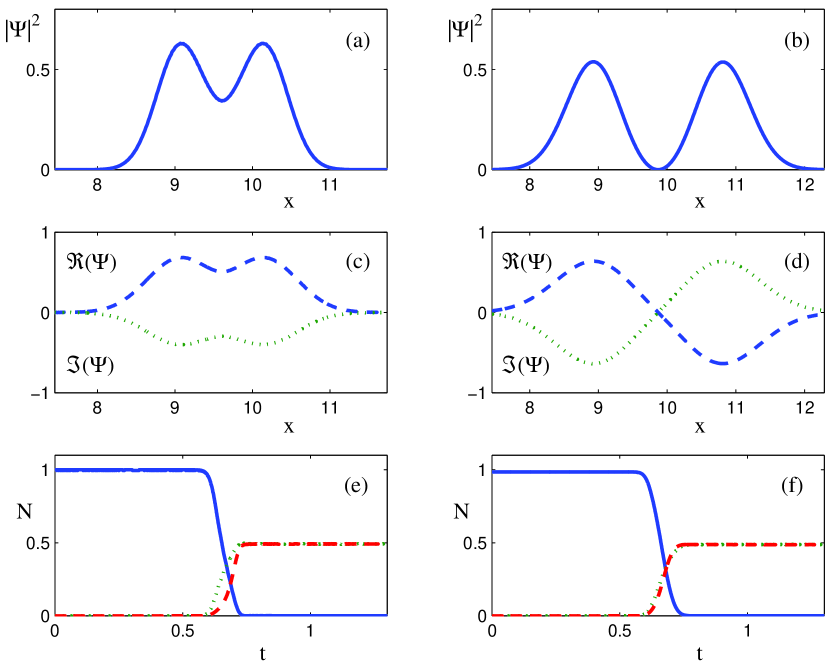
Figure 2: Wavefunctions at the end of the transfer process for the symmetric (left column) and the anti-symmetric (right column) case. The panels (a) and (b) show the density and the panels (c) and (d) show the real (broken line) and the imaginary part (dotted line) of the wavefunction. The symmetries are clearly distinguishable. The bottom row shows the change of population in the left trap (full line) and the two halves of the double well trap (broken line and dotted line). The spatial co-ordinate is scaled in units of $\alpha$.

To demonstrate the creation of coherent superposition states we have performed numerical integrations of the Schrödinger equation of the system, using an FFT/split-operator algorithm. At the start of each simulation the initial state is given by a Gaussian wavefunction centered in the trap on the left hand side and the distance between the two traps in the double well is given by $d_{R}=1.5\alpha_{R}$. Typical results are shown in Fig. 2, where the time delay between the approach sequences is given by 10% of the time for each approach process, which was in turn chosen to be $T=(1.3\Omega_{R})^{-1}$. The time dependence of the distance between the traps is chosen according to eq. (1) and the minimum distance between the traps is fixed at 1.2 $\max(\alpha,\alpha_{R})$, to make sure tunneling is the only method for transfer. The three panels on the left correspond to the case $\omega_{R}>\omega$ and the three panels on the right to the case $\omega_{R}<\omega$. The even and odd symmetries, respectively, of the final wavefunction are clearly visible. The two panels in the bottom row show the amount of $|\psi|^{2}$ in each trap. While at the beginning the wavefunction is completely localised in the trap on the left, at the end of the process it is equally split between the two wells of the double trap. There is never any significant population in the middle trap (not shown). We have performed these simulations for a wide range of values for $d_{R}$ and the delay interval, $\Delta t$, and found this process to be extremely robust.

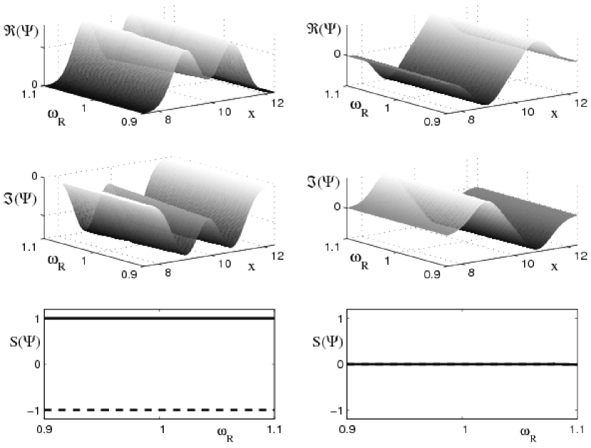
Figure 3: The four upper panels show the real and imaginary parts of the final wavefunction as a function of the trapping frequency in the double well trap. The trap frequency $\omega_{R}$ is normalised to the value required by the resonance condition and it is varied in an interval of $\pm$10%. The two graphs on the left correspond to the case $\omega<\omega_{R}$ and the two on the right to $\omega>\omega_{R}$. The two panels in the bottom row show the symmetry function for the wavefunctions above as defined in eq. (9), where the full line represents the real parts and the broken line the imaginary parts. Both lines are lying on top of each other for the antisymmetric case.

To examine the systems fragility to noise, we simulate the process above using a frequency range for $\omega_{R}$ that is $\pm$ 10% out of resonance with the value that the symmetric or the antisymmetric resonance condition (3) demands. In Fig. 3 the upper two panels on the left (right) show the real and imaginary parts of the final wavefunction for $\omega_{R}>\omega$ ($\omega_{R}<\omega$). While the transferred amount is no longer 100% (however, it is still $>99$%) for the non-resonant systems, one can immediately see that the symmetry is still a preserved property. To quantify the symmetry we define the following functions

$$S_{R}=\frac{\sum_{z}\Re(\psi(z))}{\sum_{z}|\Re(\psi(z))|}\qquad,\qquad S_{I}=\frac{\sum_{z}\Im(\psi(z))}{\sum_{z}|\Im(\psi(z))|}\;,$$ (9)

which give $S_{R,I}=\pm 1$ (depending on the phase of the wavefunction) for a perfectly symmetric state and $S_{R,I}=0$ for a perfectly antisymmetric state. The lowest panel on the left (right) hand side shows this function for $\omega_{R}>\omega$ ($\omega_{R}<\omega$) and confirms the optical inspection of the upper panels that the symmetry of the wavefunction is very robust against imperfections in the setup.

The condition that the transfer has to be performed adiabatically is already inherent in the name STIRAP. The whole process therefore has to proceed slower than the inverse of the lowest trapping frequency to avoid excitations of higher lying levels

$$T+\Delta t>\frac{1}{\min[\omega,\omega_{R}]}\;.$$ (10)

For our setup, which includes the double trap, this condition only ensures that a full transfer will be achieved from the left trap into the double well trap. In order to achieve a steady state with the desired symmetry, a second condition on the timescale has to be fulfilled, which ensures that the process is slow with respect to the tunneling frequency between the two wells in the double well trap

$$T+\Delta t>\frac{1}{\Omega_{R}}\;.$$ (11)

If this condition is not fulfilled, the final state will no longer be an eigenstate but rather be given by an oscillating population imbalance between the two wells. This, however, does not affect the symmetry of the final state. In Fig. 4 we show the amplitude of the oscillations $\Delta\rho_{A}=\max(\rho_{L}-\rho_{R})$ for different values of $T_{0}=T+\Delta t$. It can be clearly seen that a steady state is established once condition (11) is fulfilled. While the data shown are for the case $\omega>\omega_{R}$, the behaviour is analogous for $\omega<\omega_{R}$.

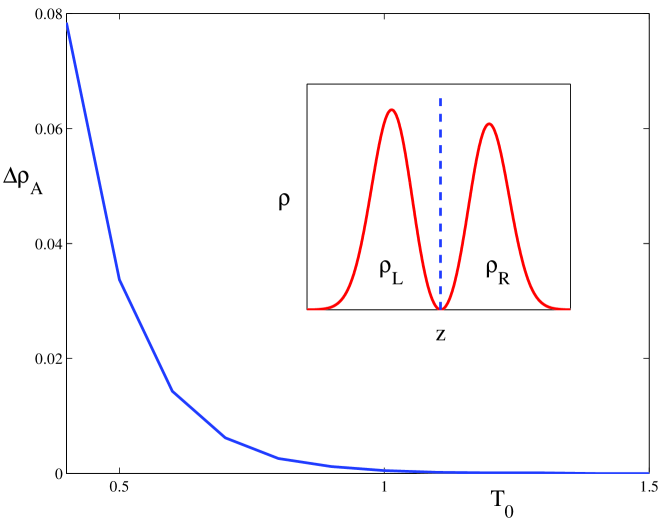
Figure 4: Oscillating density imbalance between the two halves of the double well trap, $\Delta\rho_{A}=\max(\rho_{L}-\rho_{R})$. The curve is for the anti-symmetric situation and plotted against the time interval of the process in units of $\frac{1}{\Omega_{R}}$. The inset shows an imbalanced wavefunction for which $\rho_{L}$ and $\rho_{R}$ describe the density fractions towards the left and the right from the center of the trap respectively.

The above process shows that spatial STIRAP-like processes do not only allows for a robust transport or preparation of the wavefunctions amplitude, but also allow for high fidelity when controlling the phase. It is therefore a good starting point for many applications in atom interferometry Zhang:06 . The possibility of manipulating the parts of the wavefunction selectively with well-focused laser beams and closing the interferometer by running the whole process in reverse then opens the possibility of creating universal quantum gates Englert:01 .

Schemes like this pose a challenge to current technologies, since they require dynamical control over the position of the micro-traps. Several different technologies have recently emerged that allow for such control and active experimental efforts are undertaken in many laboratories. Initial experiments have already shown the possibility of dynamically controlling the distance between traps Boyer:06 .

In summary we have suggested a robust and straightforward technique for the controlled creation of center-of-mass superposition states of atoms in micro-traps. By adjusting the trapping frequencies the final wavefunction can be chosen to be symmetric or antisymmetric. This process relies on a STIRAP-like method for transferring the atom into the new state, and the appropriate adjustment of trapping frequencies in order to choose the symmetry. While the spatial STIRAP process has been shown to be very robust for transfer of amplitudes, we have shown that it can also be used to create a very robust technique to control the phase of the wavefunction.

- (1) W. Hänsel, J. Reichel, P. Hommelhoff, and T.W. Hänsch, Phys. Rev. A 64 063607 (2001).
- (2) S. Bergamini, B. Darquié, M. Jones, L. Jacubowiez, A. Browaeys, and P. Grangier, J. Opt. Soc. Am. B 21, 1889 (2004).
- (3) C.-S. Chuu, F. Schreck, T.P. Meyrath, J.L. Hanssen, G.N. Price, and M.G. Raizen, Phys. Rev. Lett. 95, 260403 (2005).
- (4) A. Shevchenko, M. Heiliö, T. Lindvall, A. Jaakkola, I. Tittonen, M. Kaivola and T. Pfau, Phys. Rev. A 73, 051401(R) (2006).
- (5) J. Eschner, Ch. Raab, F. Schmidt-Kaler, and R. Blatt, Nature 413, 495 (2001).
- (6) J. Beugnon, M.P.A. Jones, J. Dingjan, B. Darquié, G. Messin, A. Browaeys, and P. Grangier, Nature 440, 779 (2006).
- (7) G.K. Brennen, C.M. Caves, P.S. Jessen, and I.H. Deutsch, Phys. Rev. Lett. 82, 1060 (1999).
- (8) D. Jaksch, H.-J. Briegel, J.I. Cirac, C.W. Gardiner, and P. Zoller, Phys. Rev. Lett. 82, 1975 (1999).
- (9) D. Jaksch, J.I. Cirac, P. Zoller, S.L. Rolston, R. Côté, and M.D. Lukin, Phys. Rev. Lett. 85, 2208 (2000).
- (10) G. Birkl, F.B.J. Buchkremer, R. Dumke and W. Ertmer, Opt. Comm. 191, 67 (2001).
- (11) M. Khudaverdyan, W. Alt, I. Dotsenko, L. Förster, S. Kuhr, D. Meschede, Y. Miroshnychenko, D. Schrader, and A. Rauschenbeutel, Phys. Rev. A 71, 031404(R) (2005).
- (12) D.D. Yavuz, P.B. Kulatunga, E. Urban, T.A. Johnson, N. Proite, T. Henage, T.G. Walker, and M. Saffman, Phys. Rev. Lett. 96, 063001 (2006).
- (13) Y.R.P. Sortais, H. Marion, C. Tuchendler, A.M. Lance, M. Lamare, P. Fournet, C. Armellin, R. Mercier, G. Messin, A. Browaeys, and P. Grangier, quant-ph/0610071 (2006).
- (14) M. Zhang, P. Zhang, M.S. Chapman, and L. You, Phys. Rev. Lett. 97, 070403 (2006).
- (15) K. Eckert, M. Lewenstein, R. Corbalán, G. Birkl, W. Ertmer, and J. Mompart, Phys. Rev. A 70, 023606 (2004).
- (16) K. Eckert, J. Mompart, R. Corbalán, M. Lewenstein and G. Birkl, Opt. Comm. 264, 264 (2006).
- (17) J. Arlt, K. Dholakia, J. Soneson, and E.M. Wright, Phys. Rev. A 63, 063602 (2001).
- (18) K. Brugger, P. Krüger, X. Luo, S. Wildermuth, H. Gimpel, M.W. Klein, S. Groth, R. Folman, I. Bar-Joseph, and J. Schmiedmayer, Phys. Rev. A 72, 023607 (2005).
- (19) J. Mompart, K. Eckert, W. Ertmer, G. Birkl, and M. Lewenstein, Phys. Rev. Lett. 90, 147901 (2003).
- (20) A.D. Greentree, J.H. Cole, A.R. Hamilton, and L.C.L. Hollenberg, Phys. Rev. B 70, 235317 (2004).
- (21) K. Bergmann, H. Theuer, and B.W. Shore, Rev. Mod. Phys. 70, 1003 (1998).
- (22) N.V. Vitanov, M. Fleischhauer, B.W. Shore, K. Bergmann, Adv. At., Mol., Opt. Phys. 46, 55 (2001).
- (23) Y. Niu, S. Gong, R. Li, and S. Jin, Phys. Rev. A 70, 023805 (2004).
- (24) Since the dynamics in our process can be arranged to lie in a single plane, the restriction to one-dimension for computational purposes does not have any implications for the generality of our method.
- (25) B.-G. Englert, C. Kurtsiefer, and H. Weinfurter, Phys. Rev. A 63, 032303 (2001).
- (26) V. Boyer, R.M. Godun, G. Smirne, D. Cassettari, C.M. Chandrashekar, A.B. Deb, Z.J. Laczik, and C.J. Foot, Phys. Rev. A 73, 031402 (2006).