Thermodynamic analysis of quantum light amplification

Abstract

Thermodynamics of a three-level maser was studied in the pioneering work of Scovil and Schulz-DuBois [Phys. Rev. Lett. 2, 262 (1959)]. In this work we consider the same three-level model, but treat both the matter and light quantum mechanically. Specifically, we analyze an extended (three-level) dissipative Jaynes-Cummings model (ED-JCM) within the framework of a quantum heat engine, using novel formulas for heat flux and power in bipartite systems introduced in our previous work [E. Boukobza and D. J. Tannor, PRA (in press)]. Amplification of the selected cavity mode occurs even in this simple model, as seen by a positive steady state power. However, initial field coherence is lost, as seen by the decaying off-diagonal field density matrix elements, and by the Husimi-Kano Q function. We show that after an initial transient time the field’s entropy rises linearly during the operation of the engine, which we attribute to the dissipative nature of the evolution and not to matter-field entanglement. We show that the second law of thermodynamics is satisfied in two formulations (Clausius, Carnot) and that the efficiency of the ED-JCM heat engine agrees with that defined intuitively by Scovil and Schulz-DuBois. Finally, we compare the steady state heat flux and power of the fully quantum model with the semiclassical counterpart of the ED-JCM, and derive the engine efficiency formula of Scovil and Schulz-DuBois analytically from fundamental thermodynamic fluxes.

I Introduction

Thermodynamics of quantum-optical systems has intrigued scientists ever since masers and lasers were realized experimentally. Scovil and Schulz-DuBois Scovil01 analyzed a three-level maser in the framework of a heat engine. Based on a Boltzmann distribution of atomic populations, they gave an intuitive definition of the engine’s efficiency, and showed it to be less than an or equal to the Carnot efficiency. Using the concept of negative temperature Purcell , and motivated by Ramsey’s Ramsey work on ’spin temperature’, Scovil and Schulz-DuBois Scovil02 extended their analysis of three level systems to cases where the reservoirs’ temperature is negative, and introduced the concept of negative efficiencies. Alicki studied a generic open quantum system coupled to heat reservoirs, and under the influence of varying external conditions (such as a time dependent field) Alicki . Alicki partitioned the energy of a quantum system into heat and work using the time dependencies of the density and Hamiltonian operators. Based on Alicki’s definitions for heat and work, Kosloff analyzed two coupled oscillators interacting with hot and cold thermal reservoirs in the framework of a heat engine, and showed that the engine’s efficiency complies with the second law of thermodynamics Kosloff01 . In later work, Geva and Kosloff studied a three-level amplifier coupled to two heat reservoirs Geva03 Geva04 . In their model the external field influences the dissipative terms, and the second law of thermodynamics is generally satisfied.

This paper is to some extent a continuation of the studies discussed in the previous paragraph. In contrast with previous work, in our approach the matter and the radiation field are treated as a bipartite system that is fully quantized, as opposed to a forced unipartite system. This treatment of the working medium (the material system) and the work source (the radiation field) on an equal footing requires some new thermodynamic developments, that we adapt from Erez02 . The general methodology is applied to an extended dissipative Jaynes-Cummings model (ED-JCM), which consists of a three-level material system coupled to two thermal heat baths and a quantized cavity mode. We show that this system provides a simple model of light amplification, which can then be analyzed using formulations of the first and second law of thermodynamics for bipartite systems. The heat flux and power calculated with this model lead to an engine efficiency that is in quantitative agreement with the efficiency formula intuitively defined by Scovil and Schulz-DuBois. A semiclassical counterpart of the ED-JCM equations is then presented and solved completely at steady state, giving the efficiency formula of Scovil and Schultz-DuBois analytically from fundamental thermodynamic fluxes.

This paper is arranged in the following manner. Section II is a brief introduction to the thermodynamics of bipartite systems. In Section III we define the ED-JCM master equation. In Section IV we present numerical results for the ED-JCM model, showing that it acts as a simple model for a quantum amplifier. In Section V we discuss the entropic behavior of the full system and its individual components, its behavior at steady state and the role of entanglement. In Section VI we give a thermodynamical analysis of the ED-JCM. We formulate the first law of thermodynamics in two different ways. We then show that the second law of thermodynamics is satisfied in two formulations (Clausius, Carnot), and that the efficiency of the ED-JCM heat engine agrees with that defined intuitively by Scovil and Schulz-DuBois. In Section VII we compare the steady state heat flux and power of the fully quantum model with a semiclassical version of the ED-JCM, and derive the engine efficiency formula of Scovil and Schulz-DuBois analytically from fundamental thermodynamic fluxes. Section VIII concludes.

II Thermodynamics of bipartite systems

A bipartite system is described by a density matrix of a $C^{m}\otimes C^{n}$ Hilbert space. The partial density matrix of one part is obtained by tracing over the other:

$$\rho_{A(B)}=\textrm{Tr}_{B(A)}\{\mbox{\boldmath$\rho_{AB}$}\}.$$ (1)

The entropy of a quantum system is given by the von Neumann entropy von Neumann :

$$S=-k_{B}\textrm{Tr}\{\rho\ln\rho\}.$$ (2)

The evolution of a bipartite system is given by the following master equation:

$$\mbox{\boldmath$\dot{\rho}_{AB}$}=\mathcal{L}_{h}[\mbox{\boldmath$\rho_{AB}$}]+\mathcal{L}_{d}[\mbox{\boldmath$\rho_{AB}$}],$$ (3)

where $\mathcal{L}_{h}[\mbox{\boldmath$\rho_{AB}$}]=-\frac{i}{\hbar}[\mbox{\boldmath$H$},\mbox{\boldmath$\rho_{AB}$}]$ is the Hamiltonian part of the Lindblad super operator, and $\mathcal{L}_{d}[\rho_{AB}]$ is the dissipative part of the Lindblad super operator. The bipartite time independent Hamiltonian is given by:

$$\mbox{\boldmath$H$}=\mbox{\boldmath$H_{A}$}+\mbox{\boldmath$H_{B}$}+\mbox{\boldmath$V_{AB}$},$$ (4)

where $\mbox{\boldmath$H_{A}$}=H_{A}\otimes\openone_{B}$ and $\mbox{\boldmath$H_{B}$}=\openone_{A}\otimes H_{B}$ are the Hamiltonians of subsystems $A$ and $B$, and $V_{AB}$ is the coupling term between them. Here and throughout the article, we use bold letters to signify operators that have a tensor product structure.

Heat flux and power of the individual parts of the system are defined by Erez02 :

$$\dot{Q}_{A(B)} \equiv \textrm{Tr}\{\mathcal{L}_{d}[\mbox{\boldmath$\rho_{AB}$}]\mbox{\boldmath$H_{A(B)}$}\}$$ (5)

$$P_{A(B)} \equiv -\frac{i}{\hbar}\textrm{Tr}\{\mbox{\boldmath$\rho_{AB}$}[\mbox{\boldmath$H_{A(B)}$},\mbox{\boldmath$V_{AB}$}]\}.$$

The energy flux of the full system is due only to the dissipative part of the Lindblad super operator:

$$\dot{E}_{AB}=\textrm{Tr}\{\mathcal{L}_{d}[\mbox{\boldmath$\rho_{AB}$}]\mbox{\boldmath$H$}\}.$$ (6)

III The ED-JCM master equation

Consider a three-level system interacting resonantly with one quantized cavity mode and two thermal photonic reservoirs as depicted in Fig. 1.

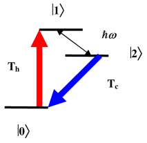
Figure 1: Three level system interacting with two heat reservoirs (hot and cold) and a quantized cavity mode.

The system is governed by the following master equation in the interaction picture:

$$\mbox{\boldmath$\dot{\rho}_{mf}$}=\mathcal{L}_{h}[\mbox{\boldmath$\rho_{mf}$}]+\mathcal{L}_{dC}[\mbox{\boldmath$\rho_{mf}$}]+\mathcal{L}_{dH}[\mbox{\boldmath$\rho_{mf}$}].$$ (7)

The letters in the subscripts have the following significance: $m$=matter, $f$=field, $d$=dissipative, $h$=Hamiltonian, $C$=cold, $H$=hot. The Hamiltonian part of the Liouvillian is given by:

$$\mathcal{L}_{h}[\mbox{\boldmath$\rho_{mf}$}]=-\frac{i}{\hbar}[\mbox{\boldmath$V_{mf}$},\mbox{\boldmath$\rho_{mf}$}],$$ (8)

where

$$\mbox{\boldmath$V_{mf}$}=\lambda(\sigma_{21}\otimes a^{{\dagger}}+\sigma_{21}^{{\dagger}}\otimes a)$$ (9)

is a resonant JCM type interaction Hamiltonian, $\lambda$ being the matter-field coupling constant. $\mathcal{L}_{dC}[\mbox{\boldmath$\rho_{mf}$}]$ and $\mathcal{L}_{dH}[\mbox{\boldmath$\rho_{mf}$}]$ are the dissipative cold and hot Lindblad super operators, respectively:

$$\!\!\!\!\!\!\!\!\!\!\!\!\!\!\!\!\!\!\!\!\!\!\!\!\!\!\!\!\!\!\!\!\!\mathcal{L}_{dC}[\mbox{\boldmath$\rho_{mf}$}] = \Gamma_{02}\{(n_{02}\!+\!1)([\mbox{\boldmath$\sigma_{02}\rho_{mf}$},\mbox{\boldmath$\sigma_{02}^{{\dagger}}$}]\!+\![\mbox{\boldmath$\sigma_{02}$},\!\mbox{\boldmath$\rho_{mf}\sigma_{02}^{{\dagger}}$}])\!+\!n_{02}([\mbox{\boldmath$\sigma_{02}^{{\dagger}}\rho_{mf}$},\mbox{\boldmath$\sigma_{02}$}]\!+\![\mbox{\boldmath$\sigma_{02}^{{\dagger}}$},\mbox{\boldmath$\rho_{mf}\sigma_{02}$}])\}$$

$$\!\!\!\!\!\!\!\!\!\!\!\!\!\!\!\!\!\!\!\!\!\!\!\!\!\!\!\!\!\!\!\!\!\mathcal{L}_{dH}[\mbox{\boldmath$\rho_{mf}$}] = \Gamma_{01}\{(n_{01}\!+\!1)([\mbox{\boldmath$\sigma_{01}\rho_{mf}$},\mbox{\boldmath$\sigma_{01}^{{\dagger}}$}]\!+\![\mbox{\boldmath$\sigma_{01}$},\mbox{\boldmath$\rho_{mf}\sigma_{01}^{{\dagger}}$}])\!+\!n_{01}([\mbox{\boldmath$\sigma_{01}^{{\dagger}}\rho_{mf}$},\mbox{\boldmath$\sigma_{01}$}]\!+\![\mbox{\boldmath$\sigma_{01}^{{\dagger}}$},\mbox{\boldmath$\rho_{mf}\sigma_{01}$}])\},$$ (10)

where $\Gamma_{02}$ and $\Gamma_{01}$ are the Weiskopf-Wigner decay constant associated with the cold and hot reservoirs, respectively, and $n_{02}$ and $n_{01}$ are the number of thermal photons in the cold and hot reservoirs, respectively. Note that direct dissipation occurs only through matter-reservoir coupling (the cold photonic reservoir couples levels $|0\rangle$ and $|2\rangle$, the hot photonic reservoir couples levels $|0\rangle$ and $|1\rangle$), and is typically used to represent atomic decay in quantum optics S&Z . The matter creation and annihilation operators are in tensor product form $\mbox{\boldmath$\sigma_{ij}$}=\sigma_{ij}\otimes\openone_{f}$, and their matrix form is given by:

$$\sigma_{21}=\left(\begin{array}[]{ccc}0&0&0\\ 0&0&0\\ 0&1&0\end{array}\right)\ \ \ \ \ \sigma_{01}=\left(\begin{array}[]{ccc}0&1&0\\ 0&0&0\\ 0&0&0\end{array}\right)\ \ \ \ \ \sigma_{02}=\left(\begin{array}[]{ccc}0&0&1\\ 0&0&0\\ 0&0&0\end{array}\right).$$

The reservoirs’ temperature is given by:

$$T_{C(H)}=\frac{\hbar\omega_{C(H)}}{k_{B}\ln(1/n_{02(01)}+1)},$$ (11)

where $\omega_{C(H)}$ is the central frequency of the cold (hot) reservoir. The ED-JCM master equation (equation 7) can be obtained by summing the Hamiltonian contribution and the two dissipative contributions. Alternatively, it can be derived for a three-level system with a break in symmetry using the weak coupling (to the reservoirs), Markovian, and Weiskopf-Wigner approximations in a similar fashion to the simple JCM with master equation with atomic damping which is derived in Appendix I.

The Hamiltonian (energy operator) of the full matter-field system is given by:

$$\mbox{\boldmath$H$}=\mbox{\boldmath$H_{m}$}+\mbox{\boldmath$H_{f}$}+\mbox{\boldmath$V_{mf}$},$$ (12)

where $\mbox{\boldmath$H_{m}$}=H_{m}\otimes\openone_{f};\ H_{m}=\hbar\sigma$ and $\mbox{\boldmath$H_{f}$}=\openone_{m}\otimes H_{f};\ H_{f}=\hbar\omega_{f}a^{{\dagger}}a$ are the matter and field Hamiltonians, respectively, and $\mathbf{\sigma}$ is given by:

$$\sigma=\left(\begin{array}[]{ccc}\omega_{0}&0&0\\ 0&\omega_{1}&0\\ 0&0&\omega_{2}\end{array}\right).$$

Under matter-field resonance ($\omega_{m}=\omega_{1}-\omega_{2}=\omega_{f}$) the Hamiltonian in the interaction picture is unchanged and is not time dependent ($\mbox{\boldmath$H^{I}$}=\mbox{\boldmath$\exp^{\frac{i}{\hbar}H_{0}t}H\exp^{-\frac{i}{\hbar}H_{0}t}$}=\mbox{\boldmath$H$};\ \mbox{\boldmath$H_{0}$}\equiv\mbox{\boldmath$H_{m}$}+\mbox{\boldmath$H_{f}$}$) since $[\mbox{\boldmath$H_{0}$},\mbox{\boldmath$V_{mf}$}]=0$ (when there is no resonance one can still transform to an interaction picture in which the Hamiltonian is unchanged Stenholm ). However, as indicated previously (eq. 8), in the interaction picture, the Hamiltonian part of the evolution of the density matrix is only via the interaction term $\mbox{\boldmath$V_{mf}$}=\mbox{\boldmath$H^{I}$}-\mbox{\boldmath$H_{0}$}$.

Before we move on to discuss the ED-JCM as a quantum amplifier, we wish to discuss the main differences between the ED-JCM and the quantum theory of the laser due to Scully and Lamb (SL) Scully00 Scully01 . Firstly, in the SL model the material system (the atom) has either four levels Scully01 or five levels S&Z , whereas in the ED-JCM the matter has three levels. Secondly, in the SL model the transitions between the two upper lasing levels and the two lower levels is achieved through a phenomenological decay, whereas in the ED-JCM population may also be pumped from the ground state to the two upper lasing levels through the full dissipative Lindblad super operator. Thirdly, in the SL model the atom is assumed to be injected into the cavity in the upper lasing level and interact with the cavity for a time $\tau$, whereas in the ED-JCM the matter is in continuous contact with the quantized cavity mode, and amplification is achieved for a wide range of initial states. Finally, in the SL model the field is allowed to decay using the Weiskopf-Wigner formalism, whereas in the ED-JCM discussed in this paper the field does not decay. In principle, cavity losses can be introduced to the ED-JCM. However, we do not consider field damping in this paper, which allows us to compare the thermodynamical fluxes in the quantum ED-JCM with their analog in a semiclassical ED-JCM (section VII) and a similar model by Geva and Kosloff in which field damping is not included Geva03 Geva04 . The differences between our model and that of the SL model will be seen below to play a crucial role in our ability to give a thermodynamic foundation of amplification.

IV The ED-JCM as a quantum amplifier

The ED-JCM master equation, eq. 7, was solved using the standard Runge-Kutta method (fourth-order Mathews ) for various choices of parameters. The accuracy of the solution was checked by decreasing the step size. Furthermore, in order to test whether the numerical solution captures all time scales (especially the rapid oscillations), the algorithm was tested on the simple JCM JCM which can be solved analytically Knight Erez01 . In all plots presented here $\Gamma_{02}=\Gamma_{01}=\Gamma=0.001,\ \lambda=1,\ n_{02}=0.1,\ n_{01}=10$, and quantities are given in atomic units. The condition $\lambda\gg\Gamma$ corresponds physically to a situation where the coupling between the matter and the selected quantized cavity mode is much stronger than the matter-reservoir coupling.

The energy flux of the full matter-field system and the individual subsystems is given by:

$$\dot{E}_{mf} \equiv \textrm{Tr}\{\mbox{\boldmath$\dot{\rho}_{mf}H$}\}=\textrm{Tr}\{\mathcal{L}_{d}[\mbox{\boldmath$\rho_{mf}$}]\mbox{\boldmath$H$}\}$$

$$\dot{E}_{m} \equiv \textrm{Tr}\{\dot{\rho}_{m}H_{m}\}=-\frac{i}{\hbar}\textrm{Tr}\{\mbox{\boldmath$\rho_{mf}$}[\mbox{\boldmath$H_{m}$},\mbox{\boldmath$V_{mf}$}]\}+\textrm{Tr}\{\mathcal{L}_{d}[\mbox{\boldmath$\rho_{mf}$}]\mbox{\boldmath$H_{m}$}\}=P_{m}+\dot{Q}_{m}$$

$$\dot{E}_{f} \equiv \textrm{Tr}\{\dot{\rho}_{f}H_{f}\}=-\frac{i}{\hbar}\textrm{Tr}\{\mbox{\boldmath$\rho_{mf}$}[\mbox{\boldmath$H_{f}$},\mbox{\boldmath$V_{mf}$}]\}=P_{f},$$ (13)

where $\dot{E}_{mf}$, $\dot{E}_{m}$, and $\dot{E}_{f}$ are the energy fluxes of the full matter-field system, the matter, and the field, respectively. $\rho_{m}$ and $\rho_{f}$ are obtained from $\rho_{mf}$ by a partial trace over the field or a partial trace over the matter, respectively. $H_{m}$ and $H_{f}$ are the Hamiltonians of the matter and field subsystems, respectively, without the tensor product with the identity. Note that the energy fluxes of the individual subsystems in eq. 13 are defined via $\rho_{m}$ and $\rho_{f}$ together with the subsystem Hamiltonians $H_{m},H_{f}$. In the next two subsections we discuss the transient and steady state energetic behavior of the ED-JCM. Since there is direct dissipation only through matter-reservoir coupling, there is no heat flux associated with the field (this is physically expected, and was shown analytically elsewhere Erez02 ).

IV.1 Transient behavior

The energy of the full matter-field system and of the individual subsystems is plotted in Fig. 2 for an initial state where the matter is in state $|1\rangle$ and the selected cavity mode has no photons ($\mbox{\boldmath$\rho_{mf}(0)$}=(|1\rangle\langle 1|)_{m}\otimes(|0\rangle\langle 0|)_{f}$).

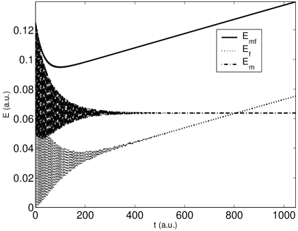
Figure 2: Energy of the full matter-field system (solid line) and the individual subsystem (field dotted line, matter dash-dot line) for an initial state where the matter is in state $|1\rangle$ and the selected cavity mode has no photons ($\mbox{\boldmath$\rho_{mf}(0)$}=(|1\rangle\langle 1|)_{m}\otimes(|0\rangle\langle 0|)_{f}$). Note that at long times there is a steady state increase in the field’s energy.

At short times, $t<\Gamma^{-1}_{eff}$, the matter and field energies oscillate at a frequency of $\Omega=\pi\lambda$ Knight . Here $\Gamma_{eff}=\Gamma\frac{n_{01}+n_{02}}{2}$ is the effective decay constant.

Moreover, at short times the well known collapse and revival phenomena Eberly Gea is observed for a sufficiently excited initial coherent state as depicted in Fig. 3.

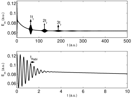
Figure 3: Matter energy at short times ($t<(2\Gamma)^{-1}$). The revival time (top) is $t_{r}=\frac{2\pi m\sqrt{\langle n\rangle}}{\lambda};\langle n\rangle=|\alpha|^{2}=100$, where $m$ is a positive integer. The Rabi oscillation time (bottom) is $t_{{\rm Rabi}}=\frac{\pi}{\lambda\sqrt{\langle n\rangle}}$.

In order to monitor the field’s coherence we calculate the quantum optical Husimi-Kano $Q$ function which is defined by Schleich :

$$Q(\alpha_{r},\alpha_{i})=\frac{1}{\pi}\langle\alpha|\rho_{f}|\alpha\rangle,$$ (14)

where $|\alpha\rangle$ is a (generally complex) coherent state. In Fig. 4 we plot the $Q$ function at four different times ($t=0$, $t=0.026\Gamma^{-1}_{eff}$, $t=0.4\Gamma_{eff}^{-1}$, $t=253\Gamma^{-1}_{eff}$) for the initial state $\mbox{\boldmath$\rho_{mf}(0)$}=(|1\rangle\langle 1|)_{m}\otimes(|\alpha\rangle\langle\alpha|)_{f}$, $|\alpha|^{2}=5$.

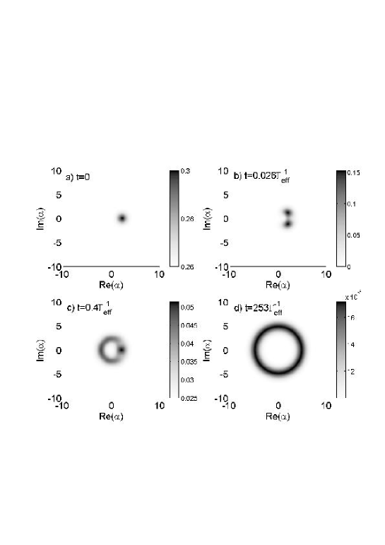
Figure 4: Husimi-Kano $Q$ function of the selected cavity mode, $\rho_{f}(0)=|\alpha\rangle\langle\alpha|;|\alpha|^{2}=5$. a): at $t=0$ the $Q$ function is a narrow 2D gaussian. b) and c): at $t=0.026\Gamma_{eff}^{-1},\ t=0.4\Gamma_{eff}^{-1}$ the $Q$ function is spread in phase space inhomogeneously. d): at $t=253\Gamma_{eff}^{-1}$ the $Q$ function has expanded (due to amplification of the selected mode) into a radially symmetric annulus (all the initial phase information is lost).

The $Q$ function at $t=0$ is that of a coherent state with the phase centered around the real axis (Fig. 4a). At transient times, the $Q$ function spreads in phase space, but it is not homogeneous as seen in Fig. 4b and Fig. 4c.

IV.2 Steady state behavior

At much longer times, $t\geq\Gamma_{eff}^{-1}$, the matter energy decreases to a steady state value, while the field energy increases with a steady state power of $P_{f}^{ss}=4.5975e^{-5}$ (the numerical value of a linear fit to the last $10000$ points, $R^{2}=1.000$) as seen in Fig. 2. Another indication for an increase in the field’s energy is seen in the steady state increase in the full system energy. Thus, the field and the matter-field system as a whole never reach a steady state for the type of evolution discussed in this paper. The relation between the full system energy and the energy of the individual component subsystems will be discussed in the next sections. A steady state increase in the field’s energy is clearly an amplification of the selected cavity mode. This behavior contrasts with the simple JCM in which the atom and field oscillate forever (the atom oscillates between the excited and ground states while the field oscillates between the $|0\rangle$ and $|1\rangle$ Fock states). Amplification of the selected cavity mode will occur with any other coherent state, including the $|0\rangle$ Fock state. The fact that the field’s energy increases monotonically is not unreasonable, since the harmonic oscillator is infinite, and since we do not consider direct dissipation of the cavity mode (which could be modeled by transmissive mirrors if desired).

The collapse and revival phenomenon at longer times is completely damped due to the dissipative contribution to the Liouvillian as seen in Fig. 3. At these long times all phase (internal coherence) information is lost: the $Q$ function is radially symmetric and is dispersed on a bigger area (bottom of Fig. 4c). From this time onwards the shape of the $Q$ function remains unchanged, and it expands fully symmetrically. The decay of the initial field coherence is also reflected in the decay of the off-diagonal field density matrix elements. At $t=10\Gamma_{eff}^{-1}$, the off-diagonal matrix elements are $10^{-13}$ times smaller than their initial value, and are practically zero. All the remaining density matrix elements are diagonal with a Poissonian-like photon distribution whose average number of photons increases with time.

The full density matrix can be divided into a $3\times 3$ block matrix, each block associated with one element of the matter density matrix. At long times, $t\geq 2\Gamma_{eff}^{-1}$, the matter-field inter-coherence is maintained by the non-vanishing matrix elements: $\rho_{1;n,2;n+1},\rho_{2;n+1,1;n}$ of the full density matrix. These elements correspond to matter-field coupling, maintained via the structure of the JCM Hamiltonian. Other density matrix elements at these long times are $5-9$ orders of magnitude smaller than the dominant non vanishing elements discussed above.

V Entropy in the ED-JCM

We consider now the entropy in the ED-JCM. In the next two subsections we discuss the transient and steady state entropic behavior. In Subsection C we discuss the relation between the entropies of the individual subsystems and entanglement, both at transient and steady state times.

V.1 Transient behavior

In Fig. 5 we plot the entropy of the full matter-field system and the individual subsystems for the initial state $\mbox{\boldmath$\rho_{mf}(0)$}=(|1\rangle\langle 1|)_{m}\otimes(|\alpha\rangle\langle\alpha|)_{f}$, $|\alpha|^{2}=25$.

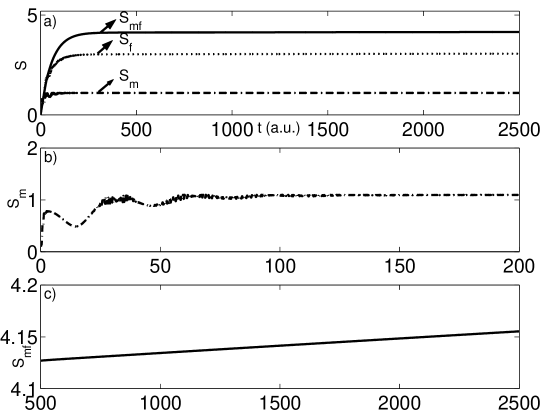
Figure 5: Entropy of the ED-JCM for the initial state $\rho_{mf}(0)=(|1\rangle\langle 1|)_{m}\otimes(|\alpha\rangle\langle\alpha|;|\alpha|^{2}=25)_{f}$. a): entropy of the full matter-field system (solid line) and the individual subsystem (field dotted line, matter dash-dot line) for the full evolution. b): matter entropy for times $t\leq\frac{\Gamma_{eff}^{-1}}{2}$. c): entropy of the full matter-field system for times $t\geq 2\Gamma_{eff}^{-1}$.

The entropy plots at the top of Fig. 5 show that there is a rapid rise ($\tau\approx\frac{\Gamma_{eff}^{-1}}{2}$) in the entropies of the matter (dash-dot line), the field (dotted line), and the full matter-field system (solid line). This overall rise in entropy is discussed in Subsection C) and is attributed to the dissipative nature of the problem.

At times $t<\Gamma_{eff}^{-1}$, the entropy of the individual subsystems (matter or field) is oscillatory, as seen by the matter entropy plot in the middle of Fig. 5. This behavior is typical of the simple JCM Knight Erez01 . At this stage $S_{m}+S_{f}>S_{mf}$; in Subsection C) we attribute the excess entropy to entanglement.

V.2 Steady state

Fig. 5a suggests that at $t>\Gamma_{eff}^{-1}$ the matter-field system has reached a steady state. Indeed, at times $t>\Gamma_{eff}^{-1}$ the energy of the matter remains constant (dash-dot line in Fig. 2). However, as was indicated in the previous section, the field energy plot (dotted line in Fig. 2) and the matter-field energy plot (solid line in Fig. 2) both show a constant rise for $t\geq\Gamma_{eff}^{-1}$. Furthermore, a closer inspection of the matter-field entropy (Fig. 5b) reveals a constant slight rise in entropy at times $t\geq\Gamma_{eff}^{-1}$ (a similar rise in the field entropy is also observed). Moreover, the field density matrix eigenvalues change in the second and third significant figures over a $\Gamma_{eff}^{-1}$ time scale. These findings give further proof of the fact that the field and matter-field system as a whole never reach a steady state.

V.3 Entanglement

We will now analyze the nature of the entropies associated with the subsystems. The entropy of the individual parts of a bipartite system is closely tied to the issue of entanglement Cerf Erez01 . An important measure for entanglement is the conditional entropy, defined for the matter-field system by:

$$S(m|f) \equiv S_{mf}-S_{f}$$

$$S(f|m) \equiv S_{mf}-S_{m},$$ (15)

where $S(m|f)$ is the conditional entropy of the matter, and $S(f|m)$ is the conditional entropy of the field. In contrast with the conditional entropy in classical bipartite systems, the conditional entropy in quantum bipartite systems can assume negative values. In this case, the correlation between the two parts of the system is of a purely quantum nature, and the system is therefore entangled. A fine example for entanglement in the context of our work is the simple JCM. Consider an initial state given by: $\mbox{\boldmath$\rho_{mf}(0)$}=(|e\rangle\langle e|)_{a}\otimes(|0\rangle\langle 0|)_{f}$, where the atom (indicated by subscript $a$) is in the excited state and the cavity mode is empty. Under the JCM Hamiltonian (pure Hamiltonian dynamics), the full atomic-field entropy is constant $S_{af}(t)=0$. However, during most of the evolution time the conditional entropies of both the atom and field (which are equal) are negative. In our case, at short times, $0<t\leq\frac{\Gamma^{-1}_{eff}}{5}$ we find that the matter’s conditional entropy is negative. Thus, the excess entropy $S_{m}+S_{f}>S_{mf}$ at these times is attributed to entanglement.

A more powerful test for entanglement, introduced originally by Peres Peres , is the negativity of the partially transposed density matrix. The partially transposed density matrix is defined by:

$$\mbox{\boldmath$\rho_{i\alpha,j\beta}^{T_{2}}$}\equiv\mbox{\boldmath$\rho_{i\beta,j\alpha}$}.$$ (16)

A sufficient condition for entanglement is the negativity of $\rho^{T_{2}}$. However, since this test applies only to finite dimensional density matrices, one should take care not to mistake truly negative eigenvalues with negative eigenvalues that are an artifact of truncation of an infinite Hilbert space Erez01 . Indeed, at times smaller than the typical decay time ($\tau=\Gamma_{eff}^{-1}$), we find that the matter-field partially transposed density matrix $\rho_{mf}^{T_{2}}$ is negative (negative eigenvalues with a substantial absolute value are found up to a time $t\approx\frac{3\Gamma_{eff}^{-1}}{4}$, and hence the matter-field system is entangled.

At $t>\Gamma_{eff}^{-1}$ the matter and field conditional entropies are positive. Moreover, the conditional entropies are almost equal to the partial entropies: $\frac{S(m|f)}{S_{m}},\frac{S(f|m)}{S_{f}}>99\%$, and $\rho_{mf}^{T_{2}}$ is positive (as was indicated before). All these findings lead us to conclude that in all likelihood at long times the matter-field system is only weakly classically correlated.

We summarize this section by stating that at short times ($t\leq\Gamma_{eff}^{-1}$), when the partial entropies are oscillatory (see bottom of Fig. 5), the matter-field system is entangled, as verified by the negative conditional entropies and the negative partially transposed full density matrix. However, as dissipation sets in, the matter-field system becomes less and less entangled. At $t>\Gamma_{eff}^{-1}$, when the partial entropies are not oscillating any more, the matter-field system in all likelihood is not entangled (as verified by the positive conditional entropies and the positive partially transposed full density matrix), and the overall rise in entropy is attributed to the dissipative Lindblad super operator.

VI Thermodynamic analysis of the steady state solution

VI.1 The first law

The first law of thermodynamics is essentially given in equation 13. However, some fine details need more clarification. The first law of thermodynamics for the full matter-field system in differential form is given by:

$$\dot{E}_{mf}\equiv\textrm{Tr}\{\mbox{\boldmath$\dot{\rho}_{mf}H$}\}=\textrm{Tr}\{\mathcal{L}_{d}[\mbox{\boldmath$\rho_{mf}$}]H\}=\dot{Q}_{m}+\dot{Q}_{f}+\dot{Q}_{V}=\dot{Q}_{m}+\dot{Q}_{V},$$ (17)

where $\dot{Q}_{f}\equiv\textrm{Tr}\{\mathcal{L}_{d}[\mbox{\boldmath$\rho_{mf}$}]\mbox{\boldmath$H_{f}$}\}=0$ as was shown elsewhere Erez02 , and $\dot{Q}_{V}\equiv\textrm{Tr}\{\mathcal{L}_{d}[\mbox{\boldmath$\rho_{mf}$}]\mbox{\boldmath$V_{mf}$}\}$. $\dot{Q}_{m}\equiv\textrm{Tr}\{\mathcal{L}_{d}[\mbox{\boldmath$\rho_{mf}$}]\mbox{\boldmath$H_{m}$}\}=\textrm{Tr}\{\mathcal{L}_{dC}[\mbox{\boldmath$\rho_{mf}$}]\mbox{\boldmath$H_{m}$}\}+\textrm{Tr}\{\mathcal{L}_{dH}[\mbox{\boldmath$\rho_{mf}$}]\mbox{\boldmath$H_{m}$}\}=\dot{Q}_{mC}+\dot{Q}_{mH}$ is the heat flux associated with the matter and it is composed of heat fluxes from/to the cold and hot heat reservoirs. Note that to an observer looking on the matter-field system as a whole, the full system is only dissipating heat.

Another way to formulate the first law of thermodynamics is based on the energy flux of individual subsystems. The first law of thermodynamics for the matter and field separately (in differential form) is given by:

$$\dot{E}_{m} \equiv \textrm{Tr}\{\dot{\rho}_{m}H_{m}\}=-\frac{i}{\hbar}\textrm{Tr}\{\mbox{\boldmath$\rho_{mf}$}[\mbox{\boldmath$H_{m}$},\mbox{\boldmath$V_{mf}$}]\}+\textrm{Tr}\{\mathcal{L}_{d}[\mbox{\boldmath$\rho_{mf}$}]\mbox{\boldmath$H_{m}$}\}=P_{m}+\dot{Q}_{m}$$ (18)

$$\dot{E}_{f} \equiv \textrm{Tr}\{\dot{\rho}_{f}H_{f}\}=-\frac{i}{\hbar}\textrm{Tr}\{\mbox{\boldmath$\rho_{mf}$}[\mbox{\boldmath$H_{f}$},\mbox{\boldmath$V_{mf}$}]\}=P_{f},$$ (19)

where $P_{m}\equiv-\frac{i}{\hbar}\textrm{Tr}\{\mbox{\boldmath$\rho_{mf}$}[\mbox{\boldmath$H_{m}$},\mbox{\boldmath$V_{mf}$}]\}$, and $P_{f}\equiv-\frac{i}{\hbar}\textrm{Tr}\{\mbox{\boldmath$\rho_{mf}$}[\mbox{\boldmath$H_{f}$},\mbox{\boldmath$V_{mf}$}]\}$ are the power terms. Since we are considering the case of perfect matter-field resonance, $P_{m}=-P_{f}$ ($[\mbox{\boldmath$H_{m}$},\mbox{\boldmath$V_{mf}$}]=-[\mbox{\boldmath$H_{f}$},\mbox{\boldmath$V_{mf}$}]$), hence:

$$\dot{E}_{m}+\dot{E}_{f}=\dot{E}_{mf}-\dot{Q}_{V}.$$ (20)

It may be shown that $\dot{Q}_{V}$ vanishes if the off-diagonal matrix elements of $\rho_{mf}$ are purely imaginary. Note that to an observer looking on the matter alone work flux (power) and heat fluxes are identified according to eq. 18, in agreement with the traditional thermodynamic partitioning of energy into work and heat. The field, which is the work source, either receives or emits energy to the working medium (the matter) in the form of power. In this paper we are interested in optical amplification. Under such conditions, at steady state the energy flux balance is such that $P_{m}^{ss}<0,\dot{Q}_{mH}>0,\dot{Q}_{mC}<0$ and the three-level system operates thermodynamically as a heat engine.

VI.2 Second law. Clausius formulation

The second law of thermodynamics is obtained via the entropy production function of the full bipartite matter-field system, which is defined by Spohn , Alicki :

$$\sigma\equiv\frac{\partial S_{mf}}{\partial t}+J,$$ (21)

where $\frac{\partial S_{mf}}{\partial t}$ is the entropy production associated with the bipartite matter-field density matrix (via differentiation of the von Neumann entropy), and $J$ is the entropy production associated with the reservoirs (via the heat flux from/to the reservoirs) given by:

$$J=-\beta_{C}\dot{Q}_{C}-\beta_{H}\dot{Q}_{H},$$ (22)

where $\beta_{C(H)}=(k_{B}T_{C(H)})^{-1}$, and $\dot{Q}_{C(H)}\equiv\textrm{Tr}\{\mathcal{L}_{dC(H)}[\mbox{\boldmath$\rho_{mf}$}](\mbox{\boldmath$H_{m}$}+\mbox{\boldmath$V_{mf}$})\}=\dot{Q}_{mC(H)}+\dot{Q}_{VC(H)}$. Spohn showed that for a completely positive map (such as the Lindblad super operator) Spohn :

$$\sigma^{Q}\geq 0.$$ (23)

Equation 23 represents the differential form of the second law of thermodynamics in Clausius’s formulation, since the sum of the entropy changes of the system and reservoirs is guaranteed to be positive.

VI.3 Second law. Carnot’s formulation

We now define a new entropy production function:

$$\sigma_{m}\equiv\frac{\partial S_{m}}{\partial t}+J_{m},$$ (24)

where $\frac{\partial S_{m}}{\partial t}$ is the entropy production associated with the matter density matrix (via differentiation of the matter von Neumann entropy), and $J_{m}$ is the entropy production associated with the reservoirs,

$$J_{m}=-\beta_{C}\dot{Q}_{mC}-\beta_{H}\dot{Q}_{mH},$$ (25)

taking into account the contribution only from the matter heat flux

$$\dot{Q}_{m}=\dot{Q}_{mC}+\dot{Q}_{mH}.$$ (26)

The physical idea behind $\sigma_{m}$ is that it is built only from matter thermodynamic fluxes: the intrinsic entropy flux $\frac{\partial S_{m}}{\partial t}$ and the entropy flux $J_{m}$ arising just from matter heat fluxes. For many initial matter states $\dot{Q}_{VC(H)}=0$ at all times, and hence $J_{m}=J$. Moreover, when the matter reaches a steady state we always find numerically (irrespective of the initial matter state) that $\dot{Q}_{VC(H)}=0$. This is the case also in the semiclassical ED-JCM discussed in section VII, where it can be shown analytically that $\dot{Q}_{VC(H)}^{ss}=0$. Therefore, at steady state, $\sigma_{m}$ is physically similar to the entropy production function in the semiclassical case, $\sigma^{SC}$, where the field is not quantized. In contrast with $\sigma^{SC}$ and $\sigma^{Q}$, $\sigma_{m}$ is not guaranteed to be positive at all times (especially at times $t<(2\Gamma)^{-1}$, due to the highly oscillatory nature of the partial entropy at short times). However, when the matter reaches a steady state ($\frac{\partial S_{m}}{\partial t}=0$), the increase in the field’s entropy is marginal (as was indicated before), and the main source of entropy production is the heat flux from/to the heat reservoirs ($J>\frac{\partial S_{mf}}{\partial t}$). Thus, when the matter reaches a steady state

$$\sigma_{m}=J_{m}=J>0,$$ (27)

and since the matter operates in a heat engine mode ($\dot{Q}_{mH}>0$ and $\dot{Q}_{mC}<0$), we obtain Carnot’s efficiency formula:

$$\eta\equiv-\frac{P_{a}}{\dot{Q}_{mH}}=\frac{\dot{Q}_{mC}+\dot{Q}_{mH}}{\dot{Q}_{mH}}\leq\frac{T_{H}-T_{C}}{T_{H}},$$ (28)

where we have used eq. 18 with eq. 26, and eq. 27 with eq. 25. For example, the efficiency of the heat engine for the choice of parameters discussed in the previous plots and for various initial field strengths (ranging from an empty cavity up to $100$ photons) is $75\%$, which is less than the Carnot efficiency which is $99\%$.

Scovil and Schulz-DuBois gave an intuitive, but non-thermodynamics definition of the efficiency of the three-level system operating as a maser Scovil01 :

$$\eta_{M}=\frac{\omega_{s}}{\omega_{p}},$$ (29)

where $\omega_{s}$ is the signal (maser) frequency, and $\omega_{p}$ is the pump frequency (central frequency of the hot reservoir, $\omega_{1}-\omega_{0}$ ). By substituting our initial choice of parameters ($\omega_{s}=\omega=0.075$, and $\omega_{p}=\omega_{1}-\omega_{0}=0.1$) we see that our numerical result agrees precisely with the efficiency estimated by Scovil and Schulz-DuBois. We find numerically that the efficiency calculated from eq. 28 agrees precisely with the efficiency calculated using eq. 29. Although we do not have analytic proof of this equivalence for the case of quantized light, we show below that this equivalence can be derived analytically when the light is treated classically.

VI.4 The ED-JCM: A work source with an entropy content

A work source is the physical entity on which work is done, or which performs work on a system (working medium). Conventional wisdom in classical thermodynamics states that a work source’s entropy is constant during the operation of a heat engine Reif . Whether the classical engine operates cyclically, as in the usual Carnot cycle, or synchronously, the working medium returns to its initial state. The working assumption in thermodynamics is that entropy may be produced at the boundary of the working medium and the heat reservoirs, but not at the boundary with the work source.

The work source in the quantum amplifier discussed in this paper is the selected cavity mode which is amplified. At steady state, the density matrix of the matter becomes constant and thus its entropy is unchanged from this time onwards. Since energy is flowing from the hot reservoir to the cold reservoir and work is produced in the form of amplification of the cavity mode, this corresponds to the engine operating in synchronous mode with the cavity mode as the work source. Inspection of Fig. 5 shows that the entropy of the light is not constant. Even after the matter reaches a steady state, the entropy of the light continues to grow linearly in time.

VII The semiclassical ED-JCM

VII.1 Equations of motion

The semiclassical ED-JCM master equation is similar to the quantum ED-JCM master equation given by equation 7. However, since the selected quantized cavity mode is replaced by a time dependent field, major differences arise. The field is considered as an external degree of freedom, and hence it has no entropy content. We propagate a $3\times 3$ density matrix representing the matter only, and all operators are represented by $3\times 3$ matrices (as opposed to $(3\otimes n)\times(3\otimes n)$ in the fully quantized case). Finally, the Hamiltonian part of the Liouvillian assumes a different form, where the creation and annihilation field operators are replaced by clockwise and anti-clockwise oscillating exponents. Despite the last difference, we note that in perfect matter-field resonance the Hamiltonian part of the Liouvillian in the interaction picture is time independent. The semiclassical Hamiltonian is given by:

$$H=H_{m}+V,$$ (30)

where $H_{m}$ is the matter Hamiltonian as given in equation 12 (without the tensor product with $\openone_{f}$), and

$$V=\lambda_{sc}(\sigma_{21}\rm{e}^{i\omega t}+\sigma_{21}^{{\dagger}}\rm{e}^{-i\omega t})$$ (31)

is the interaction Hamiltonian with a classical single coherent mode in the RWA. $\lambda_{sc}$ is the semiclassical matter-field coupling constant (which can be obtained via the semiclassical coupling matrix element Loudon ) given by (atomic units):

$$\lambda_{sc}=\mathbf{\hat{D}}\cdot\mathbf{\hat{\epsilon}}\frac{E_{0}}{2},$$ (32)

where $\mathbf{\hat{D}}$ is the dipole operator, $\mathbf{\hat{\epsilon}}$ is the field polarization, and $E_{0}$ is the field amplitude which can be estimated by calculating the average value of the quantum field operator for a coherent state Loudon :

$$E_{0}=\left(\frac{8\pi\omega}{\bar{V}}\right)^{-1/2}|\alpha|,$$ (33)

where $\omega$ is the mode frequency (not necessarily in resonance with the atomic transition), $\bar{V}$ is the cavity volume, and $|\alpha|$ is the field strength. The quantum matter-field coupling constant is given by (atomic units) Loudon :

$$\lambda=\mathbf{\hat{D}}\cdot\mathbf{\hat{\epsilon}}\left(\frac{2\pi\omega}{\bar{V}}\right)^{-1/2}.$$ (34)

Combining equations 32, 33, and 34 we obtain that:

$$\lambda_{sc}=\lambda|\alpha|.$$ (35)

The dissipative part of the Liouvillian is identical to equation 10 (without the tensor product with $\openone_{f}$).

Substitution of equation 30 and equations 10 (not in tensor product form) into equation 7 yields a set of equations for the matter density matrix elements. In the interaction picture (with $H_{0}$ given by $H_{m}$) and assuming perfect matter-field resonance, these equations take the form:

$$\dot{\rho}_{00} = 2\Gamma_{01}(n_{01}+1)\rho_{11}-2\Gamma_{01}n_{01}\rho_{00}-2\Gamma_{02}n_{02}\rho_{00}+2\Gamma_{02}(n_{02}+1)\rho_{22}$$

$$\dot{\rho}_{11} = -i\lambda_{sc}\rho_{21}+i\lambda_{sc}\rho_{12}-2\Gamma_{01}(n_{01}+1)\rho_{11}+2\Gamma_{01}n_{01}\rho_{00}$$

$$\dot{\rho}_{22} = -i\lambda_{sc}\rho_{12}+i\lambda_{sc}\rho_{21}-2\Gamma_{02}(n_{02}+1)\rho_{22}+2\Gamma_{02}n_{02}\rho_{00}$$

$$\dot{\rho}_{12} = -i\lambda_{sc}\rho_{22}+i\lambda_{sc}\rho_{11}-\Gamma_{01}(n_{01}+1)\rho_{12}-\Gamma_{02}(n_{02}+1)\rho_{12}$$

$$\dot{\rho}_{01} = i\lambda_{sc}\rho_{02}-\Gamma_{01}(2n_{01}+1)\rho_{01}-\Gamma_{02}n_{02}\rho_{01}$$

$$\dot{\rho}_{02} = i\lambda_{sc}\rho_{01}-\Gamma_{02}(2n_{02}+1)\rho_{02}-\Gamma_{01}n_{01}\rho_{02}$$

$$\dot{\rho}_{21} = \dot{\rho}_{12}^{*}$$

$$\dot{\rho}_{10} = \dot{\rho}_{10}^{*}$$

$$\dot{\rho}_{20} = \dot{\rho}_{20}^{*}.$$ (36)

VII.2 Thermodynamics of unipartite systems

Heat flux ($\dot{Q}$) and power ($P$) for unipartite systems with external (time dependent) forcing were originally defined by Alicki Alicki :

$$\dot{Q} = \textrm{Tr}\left\{\frac{\partial\rho}{\partial t}H\right\}=\textrm{Tr}\{\mathcal{L}_{d}[\rho]H\}$$ (37)

$$P = \textrm{Tr}\left\{\rho\frac{\partial H}{\partial t}\right\}.$$ (38)

VII.3 Steady state solution of the semiclassical ED-JCM

Before we derive the steady state power and heat flux we wish to discuss the main differences between the semiclassical ED-JCM and the semiclassical theory of the laser due to Lamb Lambsclaser . Firstly, in Lamb’s model the material system (the atom) has two levels, whereas in the semiclassical ED-JCM the matter has three levels. Secondly, in Lamb’s model pumping and decay of the two lasing levels are phenomenological (where the pumping function affects the field and thus the interaction term in the Hamiltonian), whereas in the semiclassical ED-JCM pumping and dumping of matter population from the ground state to the two upper lasing levels is achieved through the full dissipative Lindblad superoperator. Thirdly, in Lamb’s model the field is allowed to decay phenomenologically, whereas in the semiclassical ED-JCM discussed in this paper the field does not decay. Finally, in Lamb’s model, Maxwell’s equations for the classical field are solved self- consistently with a quantum perturbative solution of the atomic density matrix, whereas in the semiclassical ED-JCM discussed here the field is not accounted for directly. As was mentioned previously, in the semiclassical model of Geva and Kosloff the field is not accounted for directly as well. Therefore, cavity damping is not incorporated, and negative steady state power in the atom signifies an increase in the field’s energy.

The steady state solutions for $\rho_{01}$ and $\rho_{02}$ is $\rho_{01}=\rho_{02}=0$, since $\gamma\rho_{01}=0$, $\rho_{02}=\beta\rho_{01}$, and $\beta,\gamma>0$ (after applying the steady state condition $\dot{\rho}_{02}=\dot{\rho}_{01}=0$). Combining the equations for $\dot{\rho}_{12}$ and $\dot{\rho}_{21}$ at steady state ($\dot{\rho}_{12}=\dot{\rho}_{21}=0$) yields a central equation:

$$|\rho_{12}|\cos\phi(\Gamma_{01}(n_{01}+1)+\Gamma_{02}(n_{02}+1))=0,$$ (39)

where $\phi$ is the phase of the $\rho_{12}$ density matrix element. There are now three possible physical solutions.

A. $|\rho_{12}|=0$. This yields:

$$\rho_{00} = \frac{1}{1+2z}$$

$$\rho_{11} = \rho_{22}=z\rho_{00},$$ (40)

where $z=\frac{n_{01}}{n_{01}+1}=\frac{n_{02}}{n_{02}+1}$. Note that this corresponds to a very specific choice of parameters.

B. $\rm{cos}\phi=0,\ \phi=\frac{3\pi}{2}$. This yields a situation where there is no inversion of the atomic levels:

$$\rho_{11}-\rho_{22}=-\frac{|\rho_{12}|}{\lambda_{sc}}(\Gamma_{01}(n_{01}+1)+\Gamma_{02}(n_{02}+1))<0.$$ (41)

Moreover, it leads to a positive atomic steady state power which corresponds to attenuation of the electromagnetic field. This is outside the scope of the current paper, and will be explored in more detail elsewhere Erez04 .

C. $\rm{cos}\phi=0,\ \phi=\frac{\pi}{2}$. This yields a situation where there is an inversion of the atomic levels:

$$\rho_{11}-\rho_{22}=\frac{|\rho_{12}|}{\lambda_{sc}}(\Gamma_{01}(n_{01}+1)+\Gamma_{02}(n_{02}+1))>0.$$ (42)

The steady state solutions for the $\rho_{11}$, $\rho_{22}$, and $|\rho_{12}|$ density matrix elements is obtained through the solution of the following set of equations:

$$\left(\begin{array}[]{ccc}-\Gamma_{01}(2n_{01}+1)&-\Gamma_{01}n_{01}&-\lambda_{sc}\\ -\Gamma_{02}n_{02}&-\Gamma_{02}(2n_{02}+1)&\lambda_{sc}\\ \lambda_{sc}&-\lambda_{sc}&-\frac{\Gamma_{01}(n_{01}+1)+\Gamma_{02}(n_{02}+1)}{\lambda_{sc}}\\ \end{array}\right)\left(\begin{array}[]{c}\rho_{11}\\ \rho_{22}\\ |\rho_{12}|\\ \end{array}\right)=\left(\begin{array}[]{c}-\Gamma_{01}n_{01}\\ -\Gamma_{02}n_{02}\\ 0\\ \end{array}\right).$$ (43)

The solution of equation 43 can be written as:

$$\rho^{ss}=\left(\begin{array}[]{ccc}\rho_{00}&0&0\\ 0&\rho_{11}&i|\rho_{12}|\\ 0&-i|\rho_{12}|&\rho_{22}\\ \end{array}\right)=\left(\begin{array}[]{ccc}A/F&0&0\\ 0&B/F&iD/F\\ 0&-iD/F&C/F\\ \end{array}\right),$$ (44)

where $A,B,C,D,F$ are given in the Appendix II.

VII.4 Steady state heat flux and power in the semiclassical ED-JCM

We are now in position to compare the steady state heat fluxes and power of the fully quantum model with the analytical solutions of the semiclassical model. Applying Alicki’s definitions (eq. 37 and eq. 38) to the semiclassical ED-JCM at steady state yields:

$$P^{ss} = -\frac{2\Gamma_{01}\Gamma_{02}\lambda_{sc}^{3}(n_{01}-n_{02})\omega}{F}$$

$$\dot{Q}_{H}^{ss} = \frac{2\Gamma_{01}\Gamma_{02}\lambda_{sc}^{3}(n_{01}-n_{02})(\omega_{1}-\omega_{0})}{F}$$

$$\dot{Q}_{C}^{ss} = -\frac{2\Gamma_{01}\Gamma_{02}\lambda_{sc}^{3}(n_{01}-n_{02})(\omega_{2}-\omega_{0})}{F},$$ (45)

where $F=F(\Gamma_{01},\Gamma_{02},n_{01},n_{02},\lambda_{sc})$ is a positive constant given in the appendix. We note that at steady state $\textrm{Tr}\{\mathcal{L}_{dH(C)}[\rho^{ss}]V\}=0$, and thus $\dot{Q}_{H(C)}^{ss}=\textrm{Tr}\{\mathcal{L}_{dH(C)}[\rho^{ss}]H_{m}\}$.

Under the condition $\lambda\gg\Gamma$, the reservoir heat fluxes and power for the fully quantum ED-JCM are found numerically to be independent of $|\alpha|$ for the range $0\leq|\alpha|\leq 10$ (which corresponds to an initial coherent state ranging from no photons at all to $100$ photons in the cavity). There are $0.5\%$ deviations for the higher field strength range (where the initial number of photons in the cavity is close to $100$) due to a slightly rougher truncation of the Fock space.

The analytical semiclassical hot reservoir heat flux and power in the range $0.1\leq|\alpha|\leq 10$ are practically independent of $|\alpha|$, and agree almost perfectly with the numerical steady state fluxes in the fully quantum model. However, as $|\alpha|$ decreases below $0.1$ the semiclassical reservoir heat fluxes and power change dramatically. This is of course expected, as $\lambda_{sc}\propto|\alpha|$, and thus when the field’s amplitude decreases below $0.1$, $\lambda_{sc}$ is no longer much bigger than $\Gamma$. Under the condition $\lambda\gg\Gamma$, we find essentially perfect agreement between the numerical steady state fluxes of the fully quantum ED-JCM and the analytical steady state fluxes of the semiclassical ED-JCM. Therefore we can state that as far as thermodynamical fluxes are considered, the semiclassical ED-JCM captures the true physical picture. One important exception is that in the semiclassical treatment, if there is no initial field present at all ($E_{0}=0$), amplification can not take place.

For completeness, we note that the steady state amplification described above is only one of several thermodynamic modes of operation of the light-matter system. Consider the expression for the steady state power:

$$P^{ss}=\textrm{Tr}\left\{\rho^{ss}\frac{\partial V}{\partial t}\right\}=-2\lambda_{sc}\omega|\rho^{ss}_{12}|,$$ (46)

where $|\rho^{ss}_{12}|=\frac{\lambda_{sc}^{2}\Gamma_{01}\Gamma_{02}(n_{01}-n_{02})}{E}$. A mathematically feasible solution for $|\rho^{ss}_{12}|$ is obtained only when $n_{01}>n_{02}$ ($E$ is a positive constant). Substituting $|\rho^{ss}_{12}|$ into equations 42 and 46 reveals that atomic inversion and amplification go together hand in hand. Inversion in the two excited state levels implies negative power (corresponding to an amplification of the electromagnetic field) and vice versa. However, a full solution of case B reveals that $|\rho^{ss}_{12}|=-\frac{\lambda_{sc}^{2}\Gamma_{01}\Gamma_{02}(n_{01}-n_{02})}{E}$. In this case, a mathematically feasible solution for $|\rho^{ss}_{12}|$ is obtained only when $n_{02}>n_{01}$. Therefore, $|\rho^{ss}_{12}|$ is a symmetric function of $|n_{01}-n_{02}|$. The absolute value of the atomic coherence at steady state is plotted in Fig. 6 for three parameter ranges. The different thermodynamic modes of operation will be described in more detail in a forthcoming publication Erez04 .

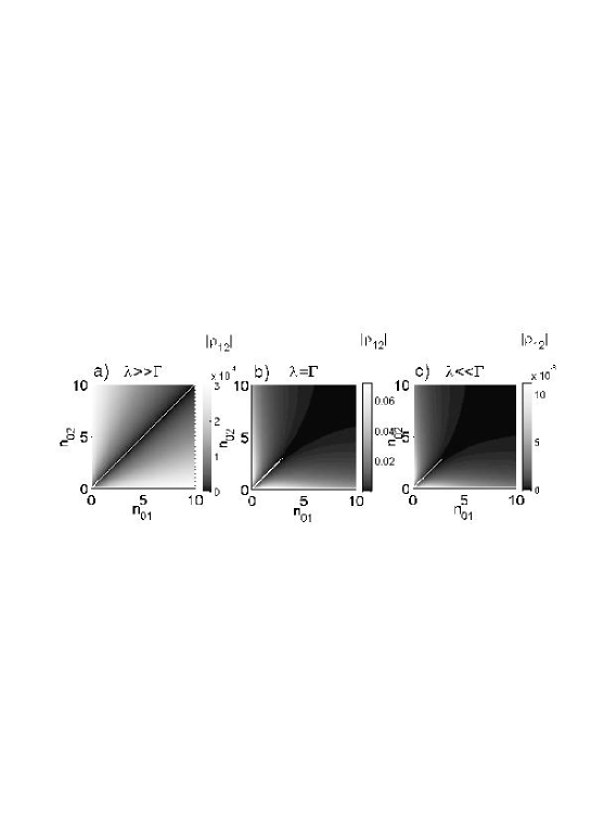
Figure 6: Semiclassical atomic coherence. a) $\lambda\gg\Gamma$. b) $\lambda=\Gamma$. c) $\lambda\ll\Gamma$.

It can be seen that substantial atomic coherence is observed only when $\lambda\approx\Gamma$.

VII.5 Engine efficiency

What about the engine’s efficiency? In the previous section we mentioned that the (numerical) efficiency of the quantum amplifier always matches the ratio obtained from Scovil and Schulz-DuBois’s intuitive definition. Before we calculate the engine’s efficiency, we wish to obtain Carnot’s formulation of the second law in differential form. We begin with Spohn’s entropy production function:

$$\sigma^{SC}=\frac{\partial S}{\partial t}-\frac{\dot{Q}_{H}}{T_{H}}-\frac{\dot{Q}_{C}}{T_{C}}\geq 0,$$ (47)

where $\frac{\partial S}{\partial t}$ is the three-level system entropy change, and $-\frac{\dot{Q}_{H(C)}}{T_{H(C)}}$ is the entropy flux from/to the hot (cold) reservoir. At steady state $\frac{\partial S}{\partial t}=0$. We now wish to rewrite $\dot{Q}_{C}^{ss}$ in terms of $\dot{Q}_{H}^{ss}$ and $P^{ss}$. The quantity $\dot{E}\equiv\textrm{Tr}\{\dot{\rho H}\}$, which measures the energy flux including the atomic-field interaction energy is given by:

$$\dot{E}=\textrm{Tr}\left\{\frac{\partial\rho}{\partial t}H\right\}+\textrm{Tr}\left\{\rho\frac{\partial H}{\partial t}\right\}=\dot{Q}_{H}+\dot{Q}_{C}+P.$$ (48)

At steady state:

$$\dot{E}^{ss}=\dot{Q}_{H}^{ss}+\dot{Q}_{C}^{ss}+P^{ss}=\frac{2\Gamma_{01}\Gamma_{02}\lambda_{sc}^{3}(n_{01}-n_{02})[\omega-(\omega_{1}-\omega_{2})]}{F}.$$ (49)

The quantity $\dot{E}^{ss}$ is zero only at perfect atomic-field resonance. However, the quantity $\dot{E}_{m}\equiv\textrm{Tr}\{\dot{\rho}H_{m}\}$, which measures the energy flux without the atomic-field interaction energy, and was introduced originally in Erez02 , is zero at steady state, as $H_{m}$ does not depend on time. Expanding $\dot{E}_{m}$ yields:

$$\dot{E}_{m}\equiv\textrm{Tr}\{\dot{\rho}H_{m}\}=\dot{Q}_{Hm}+\dot{Q}_{Cm}+P_{m},$$ (50)

where $\dot{Q}_{H(C)m}=\textrm{Tr}\{\mathcal{L}_{dH(C)}[\rho]H_{m}\}$ and $P_{m}=-\frac{i}{\hbar}\textrm{Tr}\{\rho[H_{m},V(t)]\}$ are the alternative definitions for heat flux and power introduced in Erez02 . At steady state: (1) $\dot{E}_{m}=0$ and hence $\dot{Q}_{Cm}^{ss}=-(\dot{Q}_{Hm}^{ss}+P_{m}^{ss})$, and (2) since $\textrm{Tr}\{\mathcal{L}_{dH(C)}[\rho^{ss}]V\}=0$, $\dot{Q}_{H(C)m}^{ss}=\dot{Q}_{H(C)}^{ss}$. Therefore we can replace $\dot{Q}_{C}^{ss}$ in equation 47 with $-(\dot{Q}_{H(C)}^{ss}+P_{m}^{ss})$ where

$$P_{m}^{ss}=-\frac{2\Gamma_{01}\Gamma_{02}\lambda_{sc}^{3}(n_{01}-n_{02})(\omega_{1}-\omega_{2})}{F},$$ (51)

and obtain:

$$\eta\equiv-\frac{P_{m}^{ss}}{\dot{Q}_{H}^{ss}}\leq\frac{T_{H}-T_{C}}{T_{H}},$$ (52)

which is Carnot’s efficiency formula in differential form. We note that equation 52 is always true regardless of a resonance condition. Moreover, we wish to emphasize that rewriting $\dot{Q}_{C}^{ss}$ in terms of $\dot{Q}_{H}^{ss}$ and $P_{m}^{ss}$ for non-resonant cases is possible only through the alternative approach to energy flux in unipartite systems discussed in Erez02 .

Substitution of $P_{m}^{ss}$ (which is identical with $P^{ss}$ at perfect resonance) and $\dot{Q}_{H}^{ss}$ into the engine’s efficiency formula at steady state ($\frac{\partial S_{m}}{\partial t}=0$) yields:

$$\eta=-\frac{P_{m}^{ss}}{\dot{Q}_{H}^{ss}}=\frac{\omega_{1}-\omega_{2}}{\omega_{1}-\omega_{0}}=\frac{\omega_{s}}{\omega_{p}},$$ (53)

which is identical with the maser’s efficiency defined intuitively by Scovil and Schulz-DuBois. Our model offers a statistical description for the reservoirs, and it allows us to derive thermodynamic fluxes, which in turn yield Scovil and Schulz-DuBois’s efficiency formula.

We note that Geva and Kosloff Geva04 also considered a semiclassical model for a three-level amplifier. The main difference between their model and the semiclassical ED-JCM is that in Geva and Kosloff’s model the time dependence of the classical field affects the dissipative superoperator. As a result, the steady state efficiency in the model by Geva and Kosloff depends on the power of the field, and hence it is generally not the same as in Scovil and Schulz-DuBois’s intuitive definition.

VII.6 Steady state inversion ratio

In their early work Scovil01 Scovil and Schulz-DuBois asserted that the ground state population ($\rho_{00}$) is bigger than the populations in the two excited states ($\rho_{11}$ and $\rho_{22}$). This is indeed verified in Appendix II. They also asserted that the inversion ratio between the two excited levels is given by:

$$r\equiv\frac{\rho_{11}}{\rho_{22}}=e^{-\frac{\hbar(E_{1}-E_{0})}{k_{B}T_{H}}}e^{\frac{\hbar(E_{0}-E_{2})}{k_{B}T_{C}}}=e^{-\frac{\hbar(\omega_{1}-\omega_{0})}{k_{B}T_{H}}}e^{\frac{\hbar(\omega_{0}-\omega_{2})}{k_{B}T_{C}}}.$$ (54)

This assertion appears to be well motivated physically, since it would seem that at steady state the population ratios between the two excited levels and the pumping level should be related by Boltzmann factors. However, it turns out that this is not correct. While it is true that the matter reaches a steady state, as seen in both the quantum and semiclassical models, the matter-field system as a whole does not reach a steady state, as was seen by solving the fully quantum model in this paper. Moreover, there is no a priori requirement of what steady state populations will be attained. We will now demonstrate that the ratio between the two excited levels asserted by Scovil and Schulz-DuBois is not correct. Substituting the expressions for the reservoirs’ temperatures given in equation 11 into equation 54 yields:

$$r=e^{\ln(1/n_{02}+1)}e^{-\ln(1/n_{01}+1)}=\frac{n_{01}(n_{02}+1)}{n_{02}(n_{01}+1)}.$$ (55)

Substituting $n_{01}=10,n_{02}=0.1$ yields $r=10$. In Appendix II we give analytical expressions for all the density matrix elements at steady state, from which a closed formula for $r$ may be obtained:

$$r=r(\Gamma_{01},\Gamma_{02},n_{01},n_{02},\lambda_{sc})=\frac{B}{C},$$ (56)

where $B,C$ are positive constants given in Appendix II. Substituting $n_{01}=10,n_{02}=0.1,\Gamma_{01}=\Gamma_{02}=\Gamma=0.001$ in the analytical expression for $r$ yields (similarly to the quantum model) only a marginal inversion ratio between the two excited levels, $r=\{1.01,1.00001,1.00000001\}$ for field strengths $E_{0}=\{0.1,1,10\}$, respectively, where equation 55 yields $r=10$.

VIII Conclusion

We have analyzed a fully quantum model in which a three-level material system is coupled to a single quantized cavity mode and two thermal photonic reservoirs in a framework of a heat engine. This gives what is arguably the the simplest possible quantum model for light amplification. At the same time, it permits a full thermodynamic analysis. Unlike previous work Geva04 , the field is not considered as an external time dependent force acting on the matter, but it is an integral part of the quantum system, allowing us to treat both light and matter on equal footing. We solved the ED-JCM master equation numerically, and showed that indeed amplification of the selected cavity mode occurs even in this simple model. However, initial field coherence is lost, as seen by the radially symmetric $Q$ function for $t\geq(2\Gamma)^{-1}$. Moreover, we find that the quantized field mode has an entropy content that changes dramatically at short times, and increases very slowly for $t\geq(2\Gamma)^{-1}$. The matter-field system as a whole never reaches a steady state: at $t\geq(2\Gamma)^{-1}$ the energy in the field continues to increase linearly in time, which can be analyzed thermodynamically in terms of power generation from energy in the hot reservoir. The three-level matter system, obtained by performing the partial trace of the full system over the field, does reach a steady state as seen by constant steady state energy and entropy.

Another aspect of the quantum treatment that cannot be dealt with at all within the framework of the semiclassical ED-JCM is entanglement. We showed that at short times $t<(2\Gamma)^{-1}$ the matter-field system is entangled, as seen by the negative conditional entropies and the negativity of the partially transposed density matrix. However, at longer times $t>(2\Gamma)^{-1}$ we believe that the matter-field system is classically correlated but not entangled, as the conditional entropies (which are almost equal to the partial entropies) and the partially transposed density matrix are both positive.

Based on our previous work on bipartite systems governed by a time independent master equation Erez02 we were able to derive the fundamental laws of thermodynamics. The first law is obtained both for the full matter-field system and for the individual (partially traced) subsystems, using thermodynamical fluxes of heat flux and power. The second law of thermodynamics in differential form is guaranteed to exist for the full matter-field system through Spohn’s Spohn entropy production function. We define a new entropy production function $\sigma_{m}$ based on matter thermodynamical fluxes. Through $\sigma_{m}$ we show that at steady state, when the main entropy production is due to heat fluxes from/to the heat reservoirs, Carnot’s efficiency formula is obtained in differential form.

A strong motivation for this work comes from an early paper by Scovil and Schulz-DuBois Scovil01 in which they analyze a three-level maser as a heat engine. In their work, they intuitively defined the engine’s efficiency as the ratio between the maser frequency and the pumping frequency. However, they do not connect this efficiency with explicit expressions for work and heat, as expected from a thermodynamical analysis of a heat engine. In our quantized field treatment, the efficiency formula of Scovil and Schulz-DuBois was found to be in complete agreement with numerical calculations based on thermodynamical power and heat fluxes.

We have also analyzed a semiclassical version of the ED-JCM. We obtained closed analytical expressions for power and heat flux at steady state that are in virtually perfect agreement with those obtained numerically for the fully quantum ED-JCM. One may conclude from this that as far as steady state thermodynamical fluxes are concerned, the semiclassical model is sufficient. Furthermore, from our analytical results for power and heat flux we were able to recover Scovil and Schulz-DuBois’s efficiency formula analytically. One of the assertions in the work of Scovil and Schulz-DuBois is that the ratio of populations in the two excited levels is given by a product of Boltzmann factors. We showed analytically that this last assertion does not hold in general.

In future work, we intend to explore further the other thermodynamic scenarios implied by the present model, both semiclassically and quantum mechanically. Of particular interest is the reversal of the present mode of operation of the engine so that it operates as a refrigerator for light.

Appendix I: Derivation of the damped JCM master equation

The master equation for the resonant Jaynes-Cummings model (JCM) with atomic damping in the interaction representation is given by:

$$\mbox{\boldmath$\dot{\rho}_{af}^{I}$}=\mathcal{L}_{h}[\mbox{\boldmath$\rho_{af}^{I}$}]+\mathcal{L}_{d}[\mbox{\boldmath$\rho_{af}^{I}$}],$$ (57)

where $\rho_{af}^{I}$ is the combined atom-field density matrix in the interaction picture, and $\mathcal{L}_{h}[\mbox{\boldmath$\rho_{af}^{I}$}]$ and $\mathcal{L}_{d}[\mbox{\boldmath$\rho_{af}^{I}$}]$ are given by:

$$\mathcal{L}_{h}[\mbox{\boldmath$\rho_{af}^{I}$}] = -\frac{i}{\hbar}[\mbox{\boldmath$V^{I}$},\mbox{\boldmath$\rho^{I}_{af}$}]=-i[\lambda(\mbox{\boldmath$\sigma^{-}a^{{\dagger}}$}+\mbox{\boldmath$\sigma^{+}a$}),\mbox{\boldmath$\rho^{I}_{af}$}]$$

$$\mathcal{L}_{d}[\mbox{\boldmath$\rho_{af}^{I}$}] = \!\!\Gamma(n_{th}\!+\!1)([\mbox{\boldmath$\sigma^{-}$},\mbox{\boldmath$\rho^{I}_{af}\sigma^{+}$}]\!\!+\!\![\mbox{\boldmath$\sigma^{-}\rho^{I}_{af}$},\mbox{\boldmath$\sigma^{+}$}])\!\!+\!\!\Gamma n_{th}\!([\mbox{\boldmath$\sigma^{+}$},\mbox{\boldmath$\rho^{I}_{af}\sigma^{-}$}]\!+\![\mbox{\boldmath$\sigma^{+}\rho^{I}_{af}$},\mbox{\boldmath$\sigma^{-}$}]),$$ (58)

where $\mbox{\boldmath$\sigma^{+}(a^{{\dagger}}$})$ and $\sigma^{-}(a)$ are atomic (field) creation and annihilation operators ($\mbox{\boldmath$\sigma^{+}\sigma^{-}$}-\mbox{\boldmath$\sigma^{-}\sigma^{+}$}=\mbox{\boldmath$\sigma_{z}$}$; $\sigma_{z}$ being the Pauli $z$ matrix). $\lambda$, $\Gamma$, $n_{th}$ are the atomic-field coupling constant, Weiskopf-Wigner decay constant, and the number of thermal photons, respectively. Note that since equation 57 is a master equation of a bipartite system, all the operators in equation 58 are implicitly tensor products. For example, $\sigma^{+}\sigma^{-}\rho^{I}_{af}$ is shorthand notation for $(\sigma_{+}\otimes\openone_{f})(\sigma_{-}\otimes\openone_{f})\mbox{\boldmath$\rho^{I}_{af}$}$. The damped JCM master equation is usually obtained by adding the Hamiltonian part and the dissipative part. We note that van Wonderen gave an analytical solution for the atomic density matrix in the damped JCM vanWonderen01 , and later studied the entropic behavior of the atom vanWonderen02 . In this appendix, we derive the full JCM master equation by applying the weak-coupling, Markovian and Weiskopf-Wigner approximations, and using a set of unitary transformations. The derivation of the dissipative part follows closely the derivation given by Scully and Zubairy S&Z .

We start with the full system (atom-field)-bath Hamiltonian in the Schrödinger picture:

$$\mbox{\boldmath$\hat{H}$}=\mbox{\boldmath$\hat{H}_{s}$}+\mbox{\boldmath$\hat{H}_{b}$}+\mbox{\boldmath$\hat{V}_{sb}$},$$ (59)

where $\hat{H}_{s}$, $\hat{H}_{b}$, $\hat{V}_{sb}$ are given by:

$$\hat{H}_{s} = \mbox{\boldmath$\hat{H}_{a}$}+\mbox{\boldmath$\hat{H}_{f}$}+\mbox{\boldmath$\hat{V}_{af}$}=\hbar\frac{\omega_{a}}{2}\mbox{\boldmath$\hat{\sigma}_{z}$}+\hbar\omega_{f}\mbox{\boldmath$\hat{a}^{{\dagger}}\hat{a}$}+\hbar\lambda(\mbox{\boldmath$\hat{\sigma}^{-}\hat{a}^{{\dagger}}$}+\mbox{\boldmath$\hat{\sigma}^{+}\hat{a}$})$$

$$\hat{H}_{b} = \hbar\sum_{k}{\omega_{k}\mbox{\boldmath$\hat{a}_{k}^{{\dagger}}\hat{a}_{k}$}}$$

$$\hat{V}_{sb} = \hbar\sum_{k}{\lambda_{k}(\mbox{\boldmath$\hat{\sigma}^{-}\hat{a}_{k}^{{\dagger}}$}+\mbox{\boldmath$\hat{\sigma}^{+}\hat{a}_{k}$})}.$$ (60)

We denote by $s$ the atom-field system, by $b$ the bath which is composed of an infinite number of oscillators where the operators of each oscillator are denoted by subscript $k$, and by $\lambda_{k}$ the atomic-$k$th mode coupling constant. The hat notation indicates that all operators are implicitly tensor products with the appropriate identity operators. For example $\mbox{\boldmath$\hat{\sigma}^{-}$}=\sigma^{-}\otimes\openone_{f}\otimes\openone_{b}$, $\mbox{\boldmath$\hat{a}$}=\openone_{a}\otimes a\otimes\openone_{b}$, and $\mbox{\boldmath$\hat{a}_{k}$}=\openone_{a}\otimes\openone_{f}\otimes a_{k}$. The above Hamiltonian is written under the rotating wave approximation (RWA) meaning that only energy conserving terms are considered. Note that only the atom is coupled directly to the bath modes. The evolution of the full system-bath is purely Hamiltonian:

$$\mbox{\boldmath$\dot{\rho}_{sb}$}=\mathcal{L}_{h}=-\frac{i}{\hbar}[\mbox{\boldmath$\hat{H}$},\mbox{\boldmath$\rho_{sb}$}].$$ (61)

We now move to the system-bath interaction picture (denoted by superscript $\bar{I}$):

$$\rho_{sb}^{\bar{I}} = e^{\frac{i}{\hbar}\mbox{\boldmath$\hat{\bar{H}}_{0}$}t}\mbox{\boldmath$\rho_{sb}$}e^{-\frac{i}{\hbar}\mbox{\boldmath$\hat{\bar{H}}_{0}$}t}$$

$$\dot{\rho}_{sb}^{\bar{I}} = -\frac{i}{\hbar}[\mbox{\boldmath$\hat{V}_{sb}^{\bar{I}}$},\mbox{\boldmath$\rho_{sb}^{\bar{I}}$}],$$ (62)

where:

$$\hat{\bar{H}}_{0} = \mbox{\boldmath$\hat{H}_{a}$}+\mbox{\boldmath$\hat{H}_{f}$}+\mbox{\boldmath$\hat{V}_{af}$}+\mbox{\boldmath$\hat{H}_{b}$}$$

$$\hat{V}_{sb}^{\bar{I}} = \hbar\sum_{k}{\lambda_{k}[\mbox{\boldmath$\hat{\bar{\sigma}}^{-}(t)a_{k}^{{\dagger}}$}e^{i\omega_{k}t}+\mbox{\boldmath$\hat{\bar{\sigma}}^{+}(t)a_{k}$}e^{-i\omega_{k}t}]},$$ (63)

where $\mbox{\boldmath$\hat{\bar{\sigma}}^{-(+)}(t)$}=e^{\frac{i}{\hbar}\mbox{\boldmath$\hat{H}_{s}$}t}\mbox{\boldmath$\hat{\sigma}^{-(+)}$}e^{-\frac{i}{\hbar}\mbox{\boldmath$\hat{H}_{s}$}t}$. In the derivation of equation 62 we made use of the identity $[\mbox{\boldmath$\hat{H}_{s}$},\mbox{\boldmath$\hat{H}_{b}$}]=0$. A perturbation expansion to second order in $\hat{V}_{sb}$ yields:

$$\mbox{\boldmath$\dot{\rho}_{sb}^{\bar{I}}$}=-\frac{i}{\hbar}[\mbox{\boldmath$\hat{V}_{sb}^{\bar{I}}(t)$},\mbox{\boldmath$\rho_{sb}^{\bar{I}}(0)$}]-\frac{1}{\hbar^{2}}\int_{0}^{t}{dt^{\prime}[\mbox{\boldmath$\hat{V}_{sb}^{\bar{I}}(t)$},[\mbox{\boldmath$\hat{V}_{sb}^{\bar{I}}(t^{\prime})$},\mbox{\boldmath$\rho_{sb}^{\bar{I}}(t^{\prime})$}]]}.$$ (64)

Consider the weak system-bath coupling limit, that is $\mbox{\boldmath$\rho_{sb}(t)$}=\mbox{\boldmath$\rho_{s}(t)$}\otimes\mbox{\boldmath$\rho_{b}(0)$}+\mbox{\boldmath$\rho_{c}$}$, where $\rho_{c}$ is any correlation between the system and bath which fulfills $\textrm{Tr}_{b}\{\mbox{\boldmath$\rho_{c}$}\}=0$ (this holds for $\rho_{sb}(t)$ both in the Schrödinger and interaction pictures). In this case the atom-field system evolves according to:

$$\mbox{\boldmath$\dot{\rho}_{s}^{\bar{I}}$}\equiv\textrm{Tr}_{b}\{\mbox{\boldmath$\rho_{sb}^{\bar{I}}$}\}=-\frac{i}{\hbar}\textrm{Tr}_{b}\{[\mbox{\boldmath$\hat{V}_{sb}^{\bar{I}}(t)$},\mbox{\boldmath$\rho_{s}^{\bar{I}}(0)$}\otimes\mbox{\boldmath$\rho_{b}(0)$}]\}-\frac{1}{\hbar^{2}}\textrm{Tr}_{b}\left\{\int_{0}^{t}{dt^{\prime}[\mbox{\boldmath$\hat{V}_{sb}^{\bar{I}}(t)$},[\mbox{\boldmath$\hat{V}_{sb}^{\bar{I}}(t^{\prime})$},\mbox{\boldmath$\rho_{s}^{\bar{I}}$}\otimes\mbox{\boldmath$\rho_{b}(0)$}]]}\right\}.$$ (65)

Note that in equation 65, $\mbox{\boldmath$\rho_{b}(0)$}=\mbox{\boldmath$\rho_{b}^{\bar{I}}(0)$}$ and $\mbox{\boldmath$\rho_{s}^{\bar{I}}$}=e^{\frac{i}{\hbar}\mbox{\boldmath$\hat{H}_{s}$}t}\mbox{\boldmath$\rho_{s}$}e^{-\frac{i}{\hbar}\mbox{\boldmath$\hat{H}_{s}$}t}$. The explicit form of equation 65 is given by:

$$\dot{\rho}_{s}^{\bar{I}} = -i\sum_{k}{\lambda_{k}\langle\mbox{\boldmath$\hat{a}_{k}^{{\dagger}}$}\rangle[\mbox{\boldmath$\hat{\bar{\sigma}}^{-}(t)$},\mbox{\boldmath$\rho_{s}^{\bar{I}}(0)$}]e^{i\omega_{k}t}}$$ (66)

$$- \int_{0}^{t}dt^{\prime}\sum_{k,k^{\prime}}\lambda_{k}\lambda_{k^{\prime}}\left\{[\mbox{\boldmath$\hat{\bar{\sigma}}^{-}(t)\hat{\bar{\sigma}}^{+}(t^{\prime})\rho_{s}^{\bar{I}}(t^{\prime})$}-\mbox{\boldmath$\hat{\bar{\sigma}}^{+}(t^{\prime})\rho_{s}^{\bar{I}}(t^{\prime})\bar{\sigma}_{-}(t)$}]e^{i\omega_{k}t-i\omega_{k^{\prime}}t^{\prime}}\langle\mbox{\boldmath$a_{k}^{{\dagger}}a_{k^{\prime}}$}\rangle\right.$$

$$+ [\mbox{\boldmath$\hat{\bar{\sigma}}^{+}(t)\hat{\bar{\sigma}}^{-}(t^{\prime})\rho_{s}^{\bar{I}}(t^{\prime})$}-\mbox{\boldmath$\hat{\bar{\sigma}}^{-}(t^{\prime})\rho_{s}^{\bar{I}}(t^{\prime})\bar{\sigma}^{+}(t)$}]e^{-i\omega_{k}t+i\omega_{k^{\prime}}t^{\prime}}\langle\mbox{\boldmath$a_{k}a_{k^{\prime}}^{{\dagger}}$}\rangle$$

$$+ \left.[\mbox{\boldmath$\hat{\bar{\sigma}}^{-}(t)\hat{\bar{\sigma}}^{-}(t^{\prime})\rho_{s}^{\bar{I}}(t^{\prime})$}-\mbox{\boldmath$\hat{\bar{\sigma}}^{-}(t^{\prime})\rho_{s}^{\bar{I}}(t^{\prime})\hat{\bar{\sigma}}^{-}(t)$}-\mbox{\boldmath$\hat{\bar{\sigma}}^{-}(t)\rho_{s}^{\bar{I}}(t^{\prime})\hat{\bar{\sigma}}^{-}(t^{\prime})$}\right.$$

$$+ \left.\mbox{\boldmath$\rho_{s}^{\bar{I}}(t^{\prime})\hat{\bar{\sigma}}^{-}(t^{\prime})\hat{\bar{\sigma}}^{-}(t)$}]e^{i\omega_{k}t-i\omega_{k^{\prime}}t^{\prime}}\langle\mbox{\boldmath$a_{k}^{{\dagger}}a_{k^{\prime}}^{{\dagger}}$}\rangle\right\}+\textrm{H.c.},$$

where H.c. refers to all terms on the RHS. The bath density matrix is now assumed to be composed of a product of oscillatory modes each being in a thermal state, that is:

$$\mbox{\boldmath$\rho_{b}$}=\prod_{k}{\rho_{k}};\ \rho_{k}=\sum_{n_{k}}\frac{\bar{n}_{k}^{n_{k}}}{(\bar{n}_{k}+1)^{(n_{k}+1)}}|{n_{k}}\rangle\langle{n_{k}}|,$$ (67)

where $\bar{n}_{k}$ is the average number of thermal photons in the $k$th mode. With this assumption equation 66 reduces to:

$$\dot{\rho}_{s}^{\bar{I}} = -\int_{0}^{t}dt^{\prime}\sum_{k}\lambda_{k}^{2}\left\{[\mbox{\boldmath$\bar{\sigma}^{-}(t)\bar{\sigma}^{+}(t^{\prime})\rho_{s}^{\bar{I}}(t^{\prime})$}\}-\mbox{\boldmath$\bar{\sigma}^{+}(t^{\prime})\rho_{s}^{\bar{I}}(t^{\prime})\bar{\sigma}^{-}(t)$}\}]e^{i\omega_{k}(t-t^{\prime})}\bar{n}_{k}\right.$$ (68)

$$+ \left.[\mbox{\boldmath$\bar{\sigma}^{+}(t)\bar{\sigma}^{-}(t^{\prime})\rho_{s}^{\bar{I}}(t^{\prime})$}-\mbox{\boldmath$\bar{\sigma}^{-}(t^{\prime})\rho_{s}^{\bar{I}}(t^{\prime})\bar{\sigma}^{+}(t)$}]e^{-i\omega_{1}(t-t^{\prime})}(\bar{n}_{k}+1)\right\}+\textrm{H.c.}$$ (69)

The sum over $k$ is now replaced by an integral:

$$\sum_{k}\rightarrow 2\frac{V}{(2\pi)^{3}}\int_{0}^{2\pi}d\phi\int_{0}^{\pi}d\theta\sin{\theta}\int_{0}^{\infty}d\nu_{k}\frac{\nu_{k}^{2}}{c^{3}},$$

where $V$ is the quantization volume and $\nu_{k}$ is the $k$th mode oscillation frequency. Substituting $\lambda_{k}^{2}=\frac{\nu_{k}}{2\hbar\varepsilon_{0}V}\mathcal{D}^{2}\cos^{2}{\theta}$ ($\mathcal{D}$ is the transition dipole matrix element, and $\theta$ is the angle between $\mathcal{D}$ and the electric field polarization vector), and integrating in the Weiskopf-Wigner approximation (extending the lower limit of the integral over $\nu_{k}$ from $0$ to $-\infty$, and replacing $\nu_{k}=2\pi\omega_{k}$ by $\omega$) simplifies equation 69:

$$\dot{\rho}_{s}^{\bar{I}} = \mathcal{\bar{L}}_{d}[\mbox{\boldmath$\rho_{s}^{\bar{I}}$}]=-\Gamma n_{th}[\mbox{\boldmath$\bar{\sigma}^{-}(t)\bar{\sigma}^{+}(t)\rho_{s}^{\bar{I}}(t)$}-\mbox{\boldmath$\bar{\sigma}^{+}(t)\rho_{s}^{\bar{I}}(t)\bar{\sigma}^{-}(t)$}]$$ (70)

$$- \Gamma(n_{th}+1)[\mbox{\boldmath$\bar{\sigma}^{+}(t)\bar{\sigma}^{-}(t)\rho_{s}^{\bar{I}}(t)$}-\mbox{\boldmath$\bar{\sigma}^{-}(t)\rho_{s}^{\bar{I}}(t)\bar{\sigma}^{+}(t)$}]+\textrm{H.c.},$$

where $n_{th}\equiv\bar{n}_{k_{0}}$ $(k_{0}=\omega/c)$ is the average number of thermal photons, and $\Gamma=\frac{\omega^{3}\mathcal{D}^{2}}{6\pi\hbar\varepsilon_{0}c^{3}}$ is the decay rate.

We now move to the system Schrödinger picture:

$$\rho_{s} = e^{-\frac{i}{\hbar}H_{s}t}\rho_{s}^{\bar{I}}e^{\frac{i}{\hbar}H_{s}t}$$

$$\dot{\rho}_{s} = -\frac{i}{\hbar}[\mbox{\boldmath$H_{s}$},\mbox{\boldmath$\rho_{s}$}]+\mbox{\boldmath$e^{-\frac{i}{\hbar}H_{s}t}\mathcal{\bar{L}}_{d}[\rho_{s}^{\bar{I}}]e^{\frac{i}{\hbar}H_{s}t}$}.$$ (71)

Using the definitions for $\bar{\sigma}^{-(+)}(t)$ and $\rho_{s}^{\bar{I}}$ (after tracing out the bath) it is easily shown that $\mbox{\boldmath$e^{-\frac{i}{\hbar}H_{s}t}$}\mathcal{\bar{L}}_{d}[\mbox{\boldmath$\rho_{s}^{\bar{I}}$}]\mbox{\boldmath$e^{\frac{i}{\hbar}H_{s}t}$}=\mathcal{L}_{d}[\mbox{\boldmath$\rho_{s}$}]$. Finally, the master equation for the system in the Schrödinger picture is given by:

$$\dot{\rho}_{s} = \mathcal{L}_{h}[\mbox{\boldmath$\rho_{s}$}]+\mathcal{L}_{d}[\mbox{\boldmath$\rho_{s}$}]$$

$$\mathcal{L}_{h}[\mbox{\boldmath$\rho_{s}$}] = -\frac{i}{\hbar}[\mbox{\boldmath$H_{s}$},\mbox{\boldmath$\rho_{s}$}]$$

$$\mathcal{L}_{d}[\mbox{\boldmath$\rho_{s}$}] = \Gamma(n_{th}+1)([\mbox{\boldmath$\sigma^{-}$},\mbox{\boldmath$\rho_{s}\sigma_{+}$}]+[\mbox{\boldmath$\sigma^{-}\rho_{s}$},\mbox{\boldmath$\sigma^{+}$}])+\Gamma n_{th}([\mbox{\boldmath$\sigma^{+}$},\mbox{\boldmath$\rho_{s}\sigma^{-}$}]+[\mbox{\boldmath$\sigma^{+}\rho_{s},\sigma_{-}$}]),$$ (72)

where we deliberately omitted the superscript $S$ labeling the Schrödinger picture.

To summarize, we went through the following path:

$$\mbox{\boldmath$\rho_{sb}$}\rightarrow\mbox{\boldmath$\rho_{sb}^{\bar{I}}$}\rightarrow\mbox{\boldmath$\rho_{s}^{\bar{I}}$}\rightarrow\mbox{\boldmath$\rho_{s}$}.$$

The first transition takes us from the system-bath Schrödinger picture to the system-bath interaction picture through a unitary transformation. Tracing over the bath under the weak coupling, Markovian, and Weiskopf-Wigner approximations leads us to the system dissipative interaction picture. Finally, by applying a unitary transformation we move to the system Schrödinger picture.

To complete the analysis we now move to the standard interaction picture which includes both the Hamiltonian and the dissipative parts:

$$\rho_{s}^{I} = e^{\frac{i}{\hbar}(H_{a}+H_{f})t}\rho_{s}e^{\frac{i}{\hbar}(H_{a}t+H_{f})t}$$

$$\dot{\rho}_{s}^{I} = -\frac{i}{\hbar}[\mbox{\boldmath$V$},\mbox{\boldmath$\rho_{s}^{I}$}]+\mbox{\boldmath$e^{\frac{i}{\hbar}(H_{a}+H_{f})t}$}\mathcal{L}_{d}[\mbox{\boldmath$\rho_{s}$}]\mbox{\boldmath$e^{\frac{i}{\hbar}(H_{a}+H_{f})t}$},$$ (73)

where it can be shown that: $\mbox{\boldmath$e^{-\frac{i}{\hbar}(H_{a}+H_{f})t}$}\mathcal{L}_{d}[\mbox{\boldmath$\rho_{s}$}]\mbox{\boldmath$e^{\frac{i}{\hbar}(H_{a}+H_{f})t}$}=\mathcal{L}_{d}[\mbox{\boldmath$\rho_{s}^{I}$}]$. Equation 73 is now identical with equation 58, with subscript $s$ replacing subscript $af$.

Appendix II: Density matrix of the semiclassical ED-JCM amplifier at steady state

The density matrix for the semiclassical ED-JCM operating as an amplifier ($\rho_{11}-\rho_{22}>0$) is given by:

$$\rho^{ss}=\left(\begin{array}[]{ccc}\rho_{00}&0&0\\ 0&\rho_{11}&i|\rho_{12}|\\ 0&-i|\rho_{12}|&\rho_{22}\\ \end{array}\right)=\left(\begin{array}[]{ccc}A/F&0&0\\ 0&B/F&iD/F\\ 0&-iD/F&C/F\\ \end{array}\right),$$ (74)

where $A,B,C,D,F$ are given by:

$$A = \lambda_{sc}^{3}\Gamma_{02}+\lambda_{sc}^{3}\Gamma_{01}+\lambda_{sc}^{3}\Gamma_{02}n_{02}+\lambda_{sc}^{3}\Gamma_{01}n_{01}+\Gamma_{02}\Gamma_{01}^{2}+\Gamma_{02}\Gamma_{01}^{2}n_{02}+2\Gamma_{02}\Gamma_{01}^{2}n_{01}+\Gamma_{02}\Gamma_{01}^{2}n_{01}^{2}$$

$$+ 2\Gamma_{02}\Gamma_{01}^{2}n_{02}n_{01}+\Gamma_{02}\Gamma_{01}^{2}n_{02}n_{01}^{2}+\Gamma_{02}^{2}\Gamma_{01}+2\Gamma_{02}^{2}\Gamma_{01}n_{02}+2\Gamma_{02}^{2}\Gamma_{01}n_{02}+\Gamma_{02}^{2}\Gamma_{01}n_{01}$$

$$+ 2\Gamma_{02}^{2}\Gamma_{01}n_{02}n_{01}+\Gamma_{02}^{2}\Gamma_{01}n_{02}^{2}n_{01}$$

$$B = \lambda_{sc}^{3}\Gamma_{02}n_{02}+\lambda_{sc}^{3}\Gamma_{01}n_{01}+\Gamma_{02}\Gamma_{01}^{2}n_{01}+\Gamma_{02}\Gamma_{01}^{2}n_{01}^{2}+\Gamma_{02}\Gamma_{01}^{2}n_{02}n_{01}+\Gamma_{02}\Gamma_{01}^{2}n_{02}n_{01}^{2}$$

$$+ \Gamma_{02}^{2}\Gamma_{01}n_{01}+2\Gamma_{02}^{2}\Gamma_{01}n_{02}n_{01}+\Gamma_{02}^{2}\Gamma_{01}n_{02}^{2}n_{01}$$

$$C = \lambda_{sc}^{3}\Gamma_{02}n_{02}+\lambda_{sc}^{3}\Gamma_{01}n_{01}+\Gamma_{02}\Gamma_{01}^{2}n_{02}+2\Gamma_{02}\Gamma_{01}^{2}n_{02}n_{01}+\Gamma_{02}\Gamma_{01}^{2}n_{02}n_{01}^{2}$$

$$+ \Gamma_{02}^{2}\Gamma_{01}n_{02}+\Gamma_{02}^{2}\Gamma_{01}n_{02}^{2}+\Gamma_{02}^{2}\Gamma_{01}n_{02}n_{01}+\Gamma_{02}^{2}\Gamma_{01}n_{02}^{2}n_{01}$$

$$D = \lambda_{sc}^{2}\Gamma_{02}\Gamma_{01}(n_{01}-n_{02})$$

$$F = \lambda_{sc}^{3}\Gamma_{02}+\lambda_{sc}^{3}\Gamma_{01}+3\lambda_{sc}^{3}\Gamma_{02}n_{02}+3\lambda_{sc}^{3}\Gamma_{01}n_{01}+\Gamma_{02}\Gamma_{01}^{2}+3\Gamma_{02}\Gamma_{01}^{2}n_{01}+2\Gamma_{02}\Gamma_{01}^{2}n_{01}^{2}+5\Gamma_{02}\Gamma_{01}^{2}n_{02}n_{01}$$

$$+ 3\Gamma_{02}\Gamma_{01}^{2}n_{02}n_{01}^{2}+\Gamma_{02}^{2}\Gamma_{01}+3\Gamma_{02}^{2}\Gamma_{01}n_{02}+2\Gamma_{02}^{2}\Gamma_{01}n_{02}^{2}+5\Gamma_{02}^{2}\Gamma_{01}n_{02}n_{01}+3\Gamma_{02}^{2}\Gamma_{01}n_{02}^{2}n_{01}.$$ (75)

$A,B,C,E$ are all positive constants, and since $A>B,C\Rightarrow\rho_{00}>\rho_{11},\rho_{22}$. Thus the population in the zeroth (pumping) level is always greater then the population in either level $|0\rangle$ or $|1\rangle$. Since $D/E=|\rho_{12}|$, a mathematical feasible expression is obtained only if $n_{01}>n_{02}$.

References

- (1) H. E. D. Scovil, E. O. Schulz-DuBois, Phys. Rev. Lett. 2, 262 (1959).
- (2) E. M. Purcell, R. V. Pound, Phys. Rev. 81, 279 (1951).
- (3) N. F. Ramsey, Phys. Rev. 103, 102 (1956).
- (4) J. E. Geusic, E. O. Schulz-DuBois, H. E. D. Scovil, Phys. Rev. 156, 343 (1967).
- (5) R. Alicki, J. Phys. A 12, L103 (1979).
- (6) R. Kosloff, J. Chem. Phys. 80, 1625 (1984).
- (7) E. Geva, R. Kosloff, Phys. Rev. E, 49, 3903 (1994).
- (8) E. Geva, R. Kosloff, J. Chem. Phys. 104, 7681 (1996).
- (9) E. Boukobza, D. J. Tannor, to be published.
- (10) J. von Neumann, Mathematische Grundlagen der Quantenmechanik, Berlin: Springer (1932).
- (11) M. O. Scully, M. S. Zubairy, Quantum Optics, Cambridge University Press (1997).
- (12) S. Stenholm, Phys. Rep. 6, 1 (1973).
- (13) M. O. Scully, W. E. Lamb Jr., Phys. Rev. Lett. 16, 853 (1966).
- (14) M. O. Scully, W. E. Lamb Jr., Phys. Rev. 159, 208 (1967).
- (15) J. H. Mathews Numerical Methods for Mathematics, Science, and Engineering, Prentice-Hall, Inc. (1992).
- (16) E. T. Jaynes, F. W. Cummings, Proc. IEEE 51, 89 (1963).
- (17) S. J. D. Phoenix, P. L. Knight, Annals of Physics 186, 381 (1988).
- (18) E. Boukobza, D. J. Tannor, Phys. Rev. A 71, 063821 (2005).
- (19) J. H. Eberly, N. B. Narozhny, J. J. Sanchez-Mondragon, Phys. Rev. Lett. 44, 1323 (1980).
- (20) J. Gea-Banacloche, Phys. Rev. Lett. 65, 3385 (1990).
- (21) W. P. Schleich, Quantum Optics in Phase Space, WILEW-VCH Verlag Berlin GmbH (2001).
- (22) N. J. Cerf, C. Adami, Phys. Rev. Lett. 79, 5194 (1997).
- (23) A. Peres, Phys. Rev. Lett. 77, 1413 (1996).
- (24) H. Spohn, J. Math. Phys. 19, 1227 (1978).
- (25) F. Reif, Fundamentals of Statistical and Thermal Physics, McGraw-Hill (1965).
- (26) R. Loudon, The Quantum Theory of Light, Oxford University Press (1983).
- (27) W. E. Lamb Jr., Phys. Rev. 134, A1429 (1964).
- (28) E. Boukobza, D. J. Tannor, in preparation.
- (29) A. J. van Wonderen, Phys. Rev. A 56, 3116 (1997).
- (30) F. Farhadmotamed , A. J. van Wonderen, K. Lendi, J. Phys. A 31, 3395 (1998).