Thermodynamics of bipartite systems:
Application to light-matter interactions

Abstract

Heat and work for quantum systems governed by dissipative master equations with a time-dependent driving field were introduced in the pioneering work of Alicki [J. Phys. A 12, L103 (1979)]. Alicki’s work was in the Schrödinger picture; here we extend these definitions to the Heisenberg and interaction pictures. We show that in order to avoid consistency problems, the full time derivatives in the definitions for heat flux and power (work flux) should be replaced by partial time derivatives. We also present an alternative approach to the partitioning of the energy flux which differs from that of Alicki in that the instantaneous interaction energy with the external field is not included directly. We then proceed to generalize Alicki’s definition of power by replacing the original system and its external driving field with a larger, bipartite system, governed by a time-independent Hamiltonian. Using the definition of heat flux and the generalized definition of power, we derive the first law of thermodynamics in differential form, both for the full bipartite system and the partially traced subsystems. Although the second law (Clausius formulation) is satisfied for the full bipartite system, we find that in general there is no rigorous formulation of the second law for the partially traced subsystem unless certain additional requirements are met. Once these requirements are satisfied, however, both the Carnot and the Clausius formulations of the second law are satisfied. We illustrate this thermodynamic analysis on both the simple Jaynes-Cummings model (JCM) and an extended dissipative Jaynes-Cummings model (ED-JCM), which is a model for a quantum amplifier.

I Introduction

Thermodynamics of quantum systems has intrigued scientists since the early years of the development of quantum mechanics. von Neumann von Neumann defined an entropy function which is based on the density matrix, and is similar in spirit to the Gibbs entropy. It takes into account both the populations and the coherences of the density matrix. Born Born partitioned the energy of various types of quantum statistical systems into heat and work. Tolman Tolman defined an entropy function which is identical with the Gibbs entropy, and which is based on a quantum version of Boltzmann’s $H$-function. He showed that Carnot’s formula holds for a quantum canonical distribution, and that Clausius’s inequality holds in general. Scovil and Schulz-DuBois Scovil01 analyzed a three-level quantum system coupled to two thermal reservoirs. Much later, a master equation for open quantum systems in the weak coupling Markovian regime was developed by Lindblad, who showed that under a trace-preserving completely positive map the relative entropy is non-increasing Lindblad2 . Spohn defined the entropy production function, and showed it is always positive Spohn . Pusz and Wornowicz defined work in a general $C^{*}$ algebraic context for systems with varying external forces Pusz . Based on the Markovian master equation, Alicki Alicki defined work and heat for systems with time dependent Hamiltonians. The ideas of Alicki were implemented in a series of papers by Kosloff and coworkers on quantum heat engines Kosloff01 , Geva01 , Kosloff02 .

This work continues the work of Alicki. The main focus of this paper is laying the foundations for a complete thermodynamic analysis of bipartite systems, and to apply this novel approach to quantum optical systems. It is not obvious how to generalize the thermodynamic definition of Alicki to quantum optical systems, since Alicki’s definition of work presupposes a time-dependent external field, whereas in quantum optical systems the Hamiltonian is time-independent. To solve this problem, we begin by noting that the time-dependence of the Hamiltonian in the semiclassical treatment arises from the time-independent Hamiltonian in the quantum system because we are looking at only a part of the larger system. For example, in the absence of dissipation the total energy of the bipartite matter-light system is conserved, but the energy of each subsystem in general is time-dependent. If one observes the energy changing with time in one of the subsystems, there is no way of distinguishing whether this is as a result of external forcing or because the subsystem is part of the larger bipartite system. Therefore, if work can be defined for the former we can expect that it can be defined for the latter as well. The central result of this paper, eq. 45, provides precisely such an expression for the work, expressed in terms of the Hamiltonian of the full bipartite system. Inspection of this equation shows that it is not restricted to quantum optical systems, and is in fact completely general, applying to any bipartite system. Nevertheless, the application to quantum optical systems is particularly intriguing since it lays the foundation for a thermodynamic analysis of light-matter interactions in non-equilibrium systems.

In Section II.1, we review Alicki’s definition of quantum heat and work. In Section II.2 we present a minor generalization of Alicki’s definitions for unipartite systems that provides thermodynamic consistency in the Schrödinger, the Heisenberg, and the interaction pictures. In section II.3 we suggest an alternative partitioning of energy into heat and work that differs from that of Alicki and presages the bipartite formulation in Section III. In Section II.4 we analyze the different formulations of the second law for unipartite systems. Section III, on bipartite systems, is the main part of this paper. We begin with the derivation of the general formula for work flux (power) and heat flux in bipartite systems that generalizes our unipartite formulation of the first law in Section II.3. In section III.2 we show that although the second law in the Clausius formulation is satisfied for the full bipartite system, in general there is no rigorous formulation of the second law for the partially traced subsystem unless certain additional requirements are met. Once these requirements are satisfied, however, both the Carnot and the Clausius formulations of the second law are satisfied. In Section III.3 we apply the general formalism to the simple Jaynes-Cummings model (JCM) and to an extended dissipative JCM, which serves as a quantum amplifier. Section IV concludes.

II Unipartite Systems

II.1 Energy flux of systems governed by master equations

The master equation for a system coupled to thermal reservoirs in the Schrödinger picture and the Markovian regime is given by:

$$\dot{\rho}=\mathcal{L}[\rho]=\mathcal{L}_{h}[\rho]+\mathcal{L}_{d}[\rho],$$ (1)

where $\mathcal{L}[\rho]$ is a general Lindblad super operator, $\mathcal{L}_{h}[\rho]=-\frac{i}{\hbar}[H(t),\rho]$ is the Hamiltonian Liouville super operator, and $\mathcal{L}_{d}[\rho]$ is a dissipative Lindblad super operator. Based on the master equation one can calculate the average energy by:

$$\langle E\rangle=\textrm{Tr}\{\rho(t)H(t)\}.$$ (2)

Alicki Alicki partitioned the energy into heat and work by taking the time derivative of equation 2. Heat is defined by:

$$Q\equiv\int\limits_{0}^{t}\textrm{Tr}\left\{\frac{d\rho(t^{\prime})}{dt^{\prime}}H(t^{\prime})\right\}dt^{\prime},$$ (3)

where work was defined originally by Pusz and Wornowicz Pusz as:

$$W\equiv\int\limits_{0}^{t}\textrm{Tr}\left\{\rho(t^{\prime})\frac{dH(t^{\prime})}{dt^{\prime}}\right\}dt^{\prime}.$$ (4)

A consistency problem arises when one applies these definitions in the interaction picture, and one has to be careful when defining a Heisenberg picture for a system governed by dissipative evolution. Moreover, according to eq. 4 a system whose interaction with some external degree of freedom is governed by a time independent Hamiltonian does not perform any work (as in the case of quantum electrodynamics where field-matter interactions are governed by time independent Hamiltonians). These two issues will be addressed in the sections to follow this brief introduction.

II.2 Heat and work in various pictures for unipartite systems coupled to a time dependent external field

II.2.1 The Schrödinger picture

The time evolution of the average value of an operator is given by:

$$\frac{d\langle A^{S}\rangle}{dt}=\frac{d(\textrm{Tr}\{\rho^{S}A^{S}\})}{dt}=\textrm{Tr}\left\{\frac{d\rho^{S}}{dt}A^{S}\right\}+\textrm{Tr}\left\{\rho^{S}\frac{dA^{S}}{dt}\right\}=\textrm{Tr}\left\{\frac{\partial\rho^{S}}{\partial t}A^{S}\right\}+\textrm{Tr}\left\{\rho^{S}\frac{\partial A^{S}}{\partial t}\right\},$$ (5)

where in the Schrödinger picture $d\rho^{S}/dt=\partial\rho^{S}/\partial t$ and $dA^{S}/dt=\partial A^{S}/\partial t$. Consider a system whose evolution is governed by equation 1. The first term in eq. 5 becomes:

$$\textrm{Tr}\left\{\frac{\partial\rho^{S}}{\partial t}A^{S}\}=\textrm{Tr}\{\mathcal{L}[\rho^{S}]A^{S}\}=-\frac{i}{\hbar}\textrm{Tr}\{[H^{S},\rho^{S}]A^{S}\}+\textrm{Tr}\{\mathcal{L}_{d}[\rho^{S}]A^{S}\right\}.$$ (6)

Using the definition for quantum heat (eq. 3) the heat flux in the Schrödinger picture is given by:

$$\dot{Q}=\textrm{Tr}\left\{\frac{d\rho^{S}}{dt}H^{S}\right\}=\textrm{Tr}\left\{\frac{\partial\rho^{S}}{\partial t}H^{S}\right\}=\textrm{Tr}\{\mathcal{L}_{d}[\rho^{S}]H^{S}\},$$ (7)

where in the last equality we have used the fact that $\textrm{Tr}\{\mathcal{L}_{h}[\rho^{S}]H^{S}\}=0$. The power (work flux) is thus given by:

$$P\equiv\dot{W}=\textrm{Tr}\left\{\rho^{S}\frac{dH^{S}}{dt}\right\}=\textrm{Tr}\left\{\rho^{S}\frac{\partial H^{S}}{\partial t}\right\}.$$ (8)

Note that in case of only Hamiltonian dynamics there is no heat involved, and if the Hamiltonian is time independent there is no work done by the system.

II.2.2 The Heisenberg picture

Consider a system whose evolution is purely Hamiltonian:

$$\dot{\rho^{S}}=\mathcal{L}_{h}[\rho^{S}]=-\frac{i}{\hbar}[H^{S},\rho^{S}].$$ (9)

Eq. 9 can be formally integrated:

$$\rho^{S}(t)=U(t)\rho(0)U^{{\dagger}}(t),$$ (10)

where $U(t)$ is a unitary operator. If the Hamiltonian is time independent then $U(t)=\exp^{-\frac{i}{\hbar}H^{S}t}$. Otherwise, $U(t)$ is obtained by the time ordering procedure Mukamel . The essence of the Heisenberg representation is that operators ’move’ in time, and it is defined by Mukamel :

$$A^{H}\equiv U^{{\dagger}}(t)A^{S}U(t),$$ (11)

where $U(t)$ is the same unitary operator that appears in eq. 10. Note that in this case $\rho^{H}$ is time independent:

$$\dot{\rho^{H}}=\frac{i}{\hbar}U^{{\dagger}}[H^{S},\rho^{S}]U+U^{{\dagger}}\dot{\rho^{S}}U=\frac{i}{\hbar}([H^{H},\rho^{H}]-[H^{H},\rho^{H}])=0$$ (12)

Note also that if $H^{S}$ is time independent $H^{H}(t)=H^{S}(t)=H^{S}(0)$. The average value of an operator is independent of representation:

$$\langle A^{S}\rangle=\textrm{Tr}\{\rho^{S}A^{S}\}=\textrm{Tr}\{U^{{\dagger}}(t)\rho^{S}U(t)U^{{\dagger}}(t)A^{S}U(t)\}=\textrm{Tr}\{\rho^{H}A^{H}\}=\langle A^{H}\rangle.$$ (13)

Consider now a system whose evolution is governed by eq. 1. That is, its evolution is also dissipative. A solution in the form of eq. 10 can not be obtained due to the non-unitary nature of $\mathcal{L}_{d}[\rho]$. In this case $\rho^{H}$ is time dependent:

$$\dot{\rho^{H}}=\frac{i}{\hbar}U^{{\dagger}}[H^{S},\rho^{S}]U+U^{{\dagger}}\dot{\rho^{S}}U=U^{{\dagger}}\mathcal{L}_{d}[\rho^{S}]U\equiv\mathcal{L}_{d}^{H}[\rho^{H}].$$ (14)

The evolution of the density operator in the Heisenberg picture is due to the dissipative part in the master equation, while the Hamiltonian evolution is still canceled out. The time dependence of $\rho^{H}$ is not an artifact of a definition or a transformation. Consider any function of the density matrix, for example purity ($\langle\rho\rangle=\textrm{Tr}\{\rho^{2}\}$). It is obvious that under unitary evolution, purity does not change with time (as can be shown by a Taylor expansion of the density operator). However, under dissipative dynamics purity may change with time, and this should be the case in any physical picture. Therefore, when one calculates the average value of an operator there are two contributions to its evolution: the ’moving’ density operator, and the ’moving’ observable. This can be seen by:

$$\frac{d\langle A^{H}\rangle}{dt}=\frac{d(\textrm{Tr}\{\rho^{H}A^{H}\})}{dt}=\textrm{Tr}\left\{\frac{d\rho^{H}}{dt}A^{H}\right\}+\textrm{Tr}\left\{\rho^{H}\frac{dA^{H}}{dt}\right\}.$$ (15)

The first term in eq. 15 is obtained by substitution of eq. 14:

$$\textrm{Tr}\left\{\frac{d\rho^{H}}{dt}A^{H}\right\}=\textrm{Tr}\{\mathcal{L}_{d}^{H}[\rho^{H}]A^{H}\},$$ (16)

while the second term is given by:

$$\textrm{Tr}\left\{\rho^{H}\frac{dA^{H}}{dt}\right\}=\frac{i}{\hbar}\textrm{Tr}\{\rho^{H}[H^{H},A^{H}]\}+\textrm{Tr}\left\{\rho^{H}\left(\frac{\partial A}{\partial t}\right)^{H}\right\}.$$ (17)

Substituting $H^{H}$ in eq. 16 and eq. 17 shows that the definitions for heat flux and power in the Heisenberg picture are identical to those in the Schrödinger picture:

$$\textrm{Tr}\left\{\frac{d\rho^{H}}{dt}H^{H}\right\} = \textrm{Tr}\{\mathcal{L}_{d}^{H}[\rho^{H}]H^{H}\}=\textrm{Tr}\{\mathcal{L}_{d}^{S}[\rho^{S}]H^{S}\}=\dot{Q}$$ (18)

$$\textrm{Tr}\left\{\rho^{H}\frac{dH^{H}}{dt}\right\} = \textrm{Tr}\left\{\rho^{H}\left(\frac{\partial H}{\partial t}\right)^{H}\right\}=\textrm{Tr}\left\{\rho^{S}\left(\frac{\partial H}{\partial t}\right)^{S}\right\}=P.$$ (19)

Geva and Kosloff rewrite eq. 5 using the cyclic invariance of the trace. By doing this they obtain an alternative Heisenberg picture in which the observable is evolved by the dissipative part of the master equation together with the Hamiltonian part Geva00 , Kos00 :

$$\frac{d\langle A^{S}\rangle}{dt} = \textrm{Tr}\left\{\frac{\partial\rho^{S}}{\partial t}A^{S}\right\}+\textrm{Tr}\left\{\rho^{S}\frac{\partial A^{S}}{\partial t}\right\}=\textrm{Tr}\{\mathcal{L}[\rho^{S}]A^{S}\}+\textrm{Tr}\left\{\rho^{S}\frac{\partial A^{S}}{\partial t}\right\}$$

$$= \textrm{Tr}\{\rho^{S}\mathcal{L}^{\star}[A^{S}]\}+\textrm{Tr}\left\{\rho^{S}\frac{\partial A^{S}}{\partial t}\right\}=\textrm{Tr}\left\{\rho^{S}\frac{dA}{dt}\right\},$$

where:

$$\frac{dA}{dt}\equiv\mathcal{L}^{*}[A]+\frac{\partial A}{\partial t},$$ (21)

and $\mathcal{L}^{*}[A]$ is the full Lindblad super operator as a function of $A$. However, since $\rho^{S}$ still appears in eq. II.2.2 their definitions for heat flux and power Geva00 are formally equivalent with Alicki’s definitions in the Schrödinger picture:

$$\dot{Q} = \textrm{Tr}\{\rho^{S}\mathcal{L}_{d}^{*}[H]\}=\textrm{Tr}\{\mathcal{L}_{d}[\rho^{S}]H^{S}\}$$

$$P = \textrm{Tr}\left\{\rho^{S}\left(\frac{\partial H}{\partial t}\right)^{S}\right\},$$ (22)

where $\mathcal{L}_{d}^{*}[H]$ is the dissipative Lindblad super operator as a function of $H$.

II.2.3 The interaction picture

Consider the following Hamiltonian:

$$H(t)=H_{0}+V(t),$$ (23)

where $H_{0}$ is usually a simple Hamiltonian (for example the eigenenergy Hamiltonian of a system), and $V(t)$ is the coupling to some external degree of freedom or field. The interaction representation is defined by:

$$A^{I}=U_{0}^{{\dagger}}(t)A^{S}U_{0}(t),$$ (24)

where $U_{0}$ is the propagator associated with $H_{0}$. The average value of an operator is independent of any such transformation:

$$\langle A^{S}\rangle=\textrm{Tr}\{\rho^{S}A^{S}\}=\textrm{Tr}\{U_{0}^{{\dagger}}(t)\rho^{S}U_{0}(t)U_{0}^{{\dagger}}(t)A^{S}U_{0}(t)\}=\textrm{Tr}\{\rho^{I}A^{I}\}=\langle A^{I}\rangle.$$ (25)

Differentiation of $\langle A^{I}\rangle$ yields:

$$\frac{d\langle A^{I}\rangle}{dt}=\frac{d(\textrm{Tr}\{\rho^{I}A^{I}\})}{dt}=\textrm{Tr}\left\{\frac{d\rho^{I}}{dt}A^{I}\right\}+\textrm{Tr}\left\{\rho^{I}\frac{dA^{I}}{dt}\right\}.$$ (26)

Substituting eq. 24 into the two terms in eq. 26 and using the relation $\dot{U}_{0}=-\frac{i}{\hbar}H_{0}U_{0}$ yields:

$$\textrm{Tr}\left\{\frac{d\rho^{I}}{dt}A^{I}\right\} = -\frac{i}{\hbar}\textrm{Tr}\{\rho^{I}[A^{I},V^{I}]\}+\textrm{Tr}\{\mathcal{L}_{d}^{I}[\rho^{I}]A^{I}\}$$ (27)

$$\textrm{Tr}\left\{\rho^{I}\frac{dA^{I}}{dt}\right\} = \frac{i}{\hbar}\textrm{Tr}\{\rho^{I}[H_{0}^{I},A^{I}]\}+\textrm{Tr}\left\{\rho^{I}\left(\frac{\partial A}{\partial t}\right)^{I}\right\},$$ (28)

where $\mathcal{L}_{d}^{I}[\rho^{I}]$ is the dissipative Lindblad super operator in the interaction picture. Substituting $H^{I}$ into eq. 27 and eq. 28 yields:

$$\textrm{Tr}\left\{\frac{d\rho^{I}}{dt}H^{I}\right\}\!\!\! = \!\!\!-\frac{i}{\hbar}\textrm{Tr}\{\rho^{I}\![H_{0}^{I},V^{I}]\}\!\!+\!\!\textrm{Tr}\{\mathcal{L}_{d}^{I}[\rho^{I}]H^{I}\}\!\!=\!\!-\frac{i}{\hbar}\textrm{Tr}\{\rho^{S}\![H_{0}^{S},V^{S}]\}\!\!+\!\!\textrm{Tr}\{\mathcal{L}_{d}[\rho^{S}]H^{S}\}$$ (29)

$$\textrm{Tr}\left\{\rho^{I}\frac{dH^{I}}{dt}\right\}\!\! = \!\!\frac{i}{\hbar}\textrm{Tr}\{\rho^{I}[H_{0}^{I},\!\!V^{I}]\}\!\!+\!\!\textrm{Tr}\left\{\!\!\rho^{I}\!\!\left(\frac{\partial H}{\partial t}\right)^{I}\right\}\!\!=\!\frac{i}{\hbar}\textrm{Tr}\{\rho^{S}[H_{0}^{S},\!\!V^{S}]\}\!\!+\!\!\textrm{Tr}\left\{\!\rho^{S}\!\!\left(\!\!\frac{\partial H}{\partial t}\!\right)^{S}\right\}\!\!.$$ (30)

Adding eq. 29 and eq. 30 yields $dE^{S}/dt$. However, each term differs from the corresponding terms in the Schrödinger picture by $\mp i/\hbar\textrm{Tr}\{\rho^{S}[H_{0}^{S},V^{S}]\}$ (see eq. 7 and eq. 8). Thus heat and work should be redefined to avoid a consistency problem when one moves from the Schrödinger picture to the interaction picture. We redefine heat and work as follows:

$$\dot{Q}=\textrm{Tr}\left\{\frac{\partial\rho(t^{\prime})}{\partial t^{\prime}}H(t^{\prime})\right\}$$

$$P=\textrm{Tr}\left\{\rho(t^{\prime})\frac{\partial H(t^{\prime})}{\partial t^{\prime}}\right\}.$$ (31)

The definitions for heat and work in eq. 31 differ from Alicki’s definitions for heat and work (eq. 3 and eq. 4 respectively) only by replacing the full derivatives with respect to time with the partial derivatives with respect to time. This replacement is necessary as it avoids the extra commutator term $\mp i/\hbar\textrm{Tr}\{\rho^{S}[H_{0}^{S},V^{S}]\}$ which arises from the full time derivative in eq. 26.

II.3 Alternative approach to heat and work for unipartite systems coupled to a time dependent external field

Consider a unipartite system that is governed by eq. 1, and is driven by a time dependent Hamiltonian of the form of eq. 23. The energy flux of such a system is given by substitution of $H(t)$ into eq. 5 in the Schrödinger picture:

$$\dot{E}=\frac{d\langle H^{S}\rangle}{dt}=\textrm{Tr}\left\{\frac{\partial\rho^{S}}{\partial t}H^{S}\right\}+\textrm{Tr}\left\{\rho^{S}\frac{\partial H^{S}}{\partial t}\right\}.$$ (32)

The average value of the Hamiltonian ($\langle E\rangle=\textrm{Tr}\{\rho^{S}H^{S}(t)\}$) contains contributions from both the system energy and the interaction energy. Even if the system reaches a steady state ($\dot{\rho}=0$), the quantity $\dot{E}$ is not necessarily zero at steady state due to the term $\textrm{Tr}\left\{\rho^{S}\frac{\partial H^{S}}{\partial t}\right\}$. Let us consider the energy flux of the system alone ($\langle E_{0}\rangle=\textrm{Tr}\{\rho^{S}H_{0}^{S}(t)\}$):

$$\dot{E_{0}}=\frac{d\langle H_{0}^{S}\rangle}{dt}=\textrm{Tr}\left\{\frac{\partial\rho^{S}}{\partial t}H^{S}_{0}\right\}=\textrm{Tr}\{\mathcal{L}_{d}[\rho^{S}]H_{0}^{S}\}+\textrm{Tr}\{\mathcal{L}_{h}[\rho^{S}]H_{0}^{S}\}.$$ (33)

We now define heat flux by:

$$\dot{Q}_{0}\equiv\textrm{Tr}\{\mathcal{L}_{d}[\rho]H_{0}\},$$ (34)

and power by:

$$P_{0}\equiv\textrm{Tr}\{\mathcal{L}_{h}[\rho]H_{0}\}=-\frac{i}{\hbar}\textrm{Tr}\{\rho[H_{0},V(t)]\}.$$ (35)

These definitions are novel to the best of our knowledge, and have the property of being identical in all physical pictures (the expression in the Heisenberg and interaction pictures can be obtained easily through the cyclic invariance of the trace). This partitioning of the energy flux captures the spirit of Alicki’s partitioning in the sense that power is defined via the Hamiltonian superoperator and heat flux is defined via the dissipative Lindblad superoperator (although the present definition for $\dot{Q}_{0}$ involves only the bare Hamiltonian $H_{0}$ whereas Alicki’s definition for $\dot{Q}$ involves the full Hamiltonian $H=H_{0}+V(t)$). Moreover, this partitioning of the energy flux has the same structure as the partitioning we will use in section IIIA (eq. 45 and eq. 46) where the energy of a partially traced system within a bipartite system is considered. Finally, note that the quantity $\langle E_{0}\rangle$ does reach a steady state since $H_{0}$ is time independent.

II.4 The second law for unipartite systems

The ultimate test for partitioning energy should be the fulfillment of the second law. The most general formulation of the second law is that of Clausius, which states that the total entropy change of a closed system must be greater than or equal to zero. In that respect, an open system together with the reservoirs that are coupled to it is in fact closed. Thus the entropy changes of the system and of the reservoirs must fulfill the relation: $\Delta S_{total}=\Delta S_{system}+\Delta S_{reservoirs}\geq 0$. For this relation to hold there is no need to define work. When the system operates in a cycle, the only contribution to the total entropy change is the entropy change of the reservoirs ($\Delta S_{system}=0$), and one can derive a Carnot formulation of the second law, which sets a limit on the engine efficiency. However, in order to have a Carnot formulation of the second law, work must be defined.

To derive the Clausius and Carnot formulations of the non-equilibrium second law of thermodynamics in differential form, one replaces the equilibrium thermodynamic quantities of heat and work by thermodynamic currents (or fluxes) of heat flux and power. In order to satisfy Clausius’s formulation of the second law for driven unipartite systems at all times we believe that one has to use Alicki’s definition for heat flux. However, at steady state, in order to obtain Carnot’s formula one must use our definitions (especially for power), as we now explain.

We begin with Spohn’s entropy production function Spohn for a system coupled to two reservoirs:

$$\sigma=\frac{\partial S}{\partial t}-\frac{\dot{Q}_{H}}{T_{H}}-\frac{\dot{Q}_{C}}{T_{C}},$$ (36)

where $\frac{\partial S}{\partial t}$ is the system’s entropy change defined via the von Neumann entropy, and $-\frac{\dot{Q}_{H(C)}}{T_{H(C)}}$ is the reversible entropy current from/to the hot (cold) thermal reservoir. Spohn showed that for a completely positive map (such as the Lindblad super operator) Spohn :

$$\sigma\geq 0.$$ (37)

Eq. 37 is Clausius’s general formulation of the second law in differential form, which is valid at all times.

At steady state $\frac{\partial S}{\partial t}=0$, and hence we need to analyze only the thermodynamic currents from/to the reservoirs. Note that $\dot{Q}_{H(C)}=\textrm{Tr}\{\mathcal{L}_{dH(C)}[\rho]H\}$ has two contributions, namely $\dot{Q}_{H(C)}=\dot{Q}_{H(C)0}+\dot{Q}_{H(C)V}$, where $\dot{Q}_{H(C)V}=\textrm{Tr}\{\mathcal{L}_{dH(C)}[\rho]V\}$. Writing eq. 33 for the case of two reservoirs yields:

$$\dot{E}_{0}=\dot{Q}_{H0}+\dot{Q}_{C0}+P_{0}.$$ (38)

At steady state ($\dot{E}_{0}=0$), $\dot{Q}_{C0}^{ss}=-(\dot{Q}_{H0}^{ss}+P_{0}^{ss})$. If we assume that $\dot{Q}_{C(H)V}^{ss}=0$, substitution of eq. 38 into eq. 36 yields Carnot’s famous formula in differential form:

$$\eta\equiv-\frac{P_{0}}{\dot{Q}_{H0}}\leq\frac{T_{H}-T_{C}}{T_{H}}.$$ (39)

Note that a similar Carnot formulation of the second law does not generally exist using Alicki’s formalism, due to the fact that generally $\dot{E}\neq 0$, for example in the non-resonant semiclassical ED-JCM discussed in Erez03 .

For completeness, we note that if $\dot{Q}_{C(H)V}=0$, eq. 36 is trivially satisfied.

III Thermodynamics of bipartite systems with time independent Hamiltonians

III.1 Energy fluxes for bipartite systems

Consider a bipartite system whose evolution is governed by eq. 1. The time independent bipartite Hamiltonian operates in a $C^{m}\otimes C^{n}$ Hilbert space, and it is given by:

$$\mbox{\boldmath$H$}=\mbox{\boldmath$H_{A}$}+\mbox{\boldmath$H_{B}$}+\mbox{\boldmath$V_{AB}$},$$ (40)

where $\mbox{\boldmath$H_{A}$}=H_{A}\otimes\openone_{B}$ and $\mbox{\boldmath$H_{B}$}=\openone_{A}\otimes H_{B}$. For simplicity we consider direct dissipation through subsystem $A$ only. However, the analysis that follows can be generalized easily to the case where both subsystems dissipate energy directly to the environment. The generic form of the dissipative Lindblad super operator is given by:

$$\mathcal{L}_{d}[\mbox{\boldmath$\rho_{AB}$}]=\sum_{k}\Gamma_{k}\{a_{k}([\mbox{\boldmath$\sigma_{k}^{{\dagger}}$},\mbox{\boldmath$\sigma_{k}\rho_{AB}$}]+[\mbox{\boldmath$\rho_{AB}\sigma_{k}^{{\dagger}}$},\mbox{\boldmath$\sigma_{k}$}])+b_{k}([\mbox{\boldmath$\sigma_{k}$},\mbox{\boldmath$\sigma_{k}^{{\dagger}}\rho_{AB}$}]+[\mbox{\boldmath$\rho_{AB}\sigma_{k}$},\mbox{\boldmath$\sigma_{k}^{{\dagger}}$}])\}\equiv\sum_{k}\mathcal{L}_{d}^{(k)}[\mbox{\boldmath$\rho_{AB}$}],$$ (41)

where $\mbox{\boldmath$\sigma_{k}$}(\mbox{\boldmath$\sigma_{k}^{{\dagger}}$})$ is the $k$th lowering (raising) operator of subsystem $A$ in the tensor product space ($\mbox{\boldmath$\sigma_{k}$}(\mbox{\boldmath$\sigma_{k}^{{\dagger}}$})=\sigma_{kA}(\sigma_{kA}^{{\dagger}})\otimes\openone_{B}$), $\Gamma_{k}$ is the $k$th decay rate, $a_{k}$, and $b_{k}$ are prefactors whose ratio is a function of the temperature of the $k$th reservoir.

The derivation that follows is general for either the Schrödinger, Heisenberg, or interaction representation. For convenience we will work in the Schrödinger representation. Using the definition for heat flux (eq. 31), the energy flux of the full bipartite system is given by:

$$\dot{E}_{AB}=\textrm{Tr}\{\mathcal{L}_{d}[\mbox{\boldmath$\rho_{AB}$}]\mbox{\boldmath$H$}\}\equiv\dot{Q}=\sum_{k}\dot{Q}_{k},$$ (42)

where $\dot{Q}_{k}=\textrm{Tr}\{\mathcal{L}_{d}^{(k)}\mbox{\boldmath$H$}\}$ is the heat flux associated with coupling to the $k$th reservoir. Note that since the Hamiltonian is time independent there is no work involved. Thus, to an outside observer looking on the bipartite system as a whole the full system is only dissipating. Is this the whole story? No.

Let us examine the energy flux of subsystem $A$ (the subsystem for which direct dissipation occurs):

$$\dot{E}_{A}\equiv\textrm{Tr}_{A}\{\dot{\rho}_{A}H_{A}\}=\textrm{Tr}\{\mathcal{L}[\mbox{\boldmath$\rho_{AB}$}]\mbox{\boldmath$H_{A}$}\}=-\frac{i}{\hbar}\textrm{Tr}\{\mbox{\boldmath$\rho_{AB}$}[\mbox{\boldmath$H_{A}$},\mbox{\boldmath$V_{AB}$}]\}+\textrm{Tr}\{\mathcal{L}_{d}[\mbox{\boldmath$\rho_{AB}$}]\mbox{\boldmath$H_{A}$}\},$$ (43)

where $H_{A}$ is the Hamiltonian of subsystem $A$ without the tensor product with $\openone_{B}$, and $\dot{\rho}_{A}=\textrm{Tr}_{B}\{\mbox{\boldmath$\rho_{AB}$}\}$ is the partial density matrix of subsystem $A$. The first equality in equation 43 stems from the following algebra:

$$\dot{E}_{A} = \textrm{Tr}_{A}\{\dot{\rho}_{A}H_{A}\}=\sum_{i,j}{\dot{\rho}_{A}^{ij}H_{A}^{ji}}=\sum_{i,j}{(\sum_{\alpha}{\mbox{\boldmath$\dot{\rho}_{AB}^{i\alpha,j\alpha}$}})H_{A}^{ji}}$$ (44)

$$= \!\!\!\!\!\sum_{i,j,\alpha,\beta}{\mbox{\boldmath$\dot{\rho}_{AB}^{i\alpha,j\beta}$}H_{A}^{ji}\delta_{B}^{\beta\alpha}}=\sum_{i,j,\alpha,\beta}{\mbox{\boldmath$\dot{\rho}_{AB}^{i\alpha,j\beta}H_{A}^{j\beta,i\alpha}$}}=\textrm{Tr}_{A,B}\{\mbox{\boldmath$\dot{\rho}_{AB}H_{A}$}\}=\textrm{Tr}\{\mathcal{L}[\mbox{\boldmath$\rho_{AB}$}]\mbox{\boldmath$H_{A}$}\}.$$

Comparing eq. 43 and eq. 44 we associate the first term on the RHS of eq. 43 with power:

$$P_{A}\equiv-\frac{i}{\hbar}\textrm{Tr}\{\mbox{\boldmath$\rho_{AB}$}[\mbox{\boldmath$H_{A}$},\mbox{\boldmath$V_{AB}$}]\},$$ (45)

while we associate the second term with heat flux:

$$\dot{Q}_{A}\equiv\textrm{Tr}\{\mathcal{L}_{d}[\mbox{\boldmath$\rho_{AB}$}]\mbox{\boldmath$H_{A}$}\}.$$ (46)

Before we continue we wish to emphasize the differences between our novel definitions for heat flux and power (eq. 46 and eq. 45, respectively) and these of Alicki (eq. 3 and eq. 4, respectively). Firstly, our definitions refer to a single degree of freedom within a bipartite system. Secondly, the dimensionality of the operators in our definitions is $m\otimes n$ (due to the expansion in eq. 44) as opposed to $m$ when a single degree of freedom is coupled to an external field (Alicki’s work). Thirdly, power emerges simply from the commutator between $H_{A}$ and $V_{AB}$, and not from a time dependent field. The last difference is striking since it indicates that the Hamiltonian need not depend on time to get work. In fact, whenever an external field is replaced by a quantized degree of freedom, the time dependence of the Hamiltonian is removed at the expense of increasing the dimensionality of the Hamiltonian.

Similarly, we can analyze the energy flux of subsystem $B$:

$$\dot{E}_{B}\equiv\textrm{Tr}_{B}\{\dot{\rho}_{B}H_{B}\}=-\frac{i}{\hbar}\textrm{Tr}\{\mbox{\boldmath$\rho_{AB}$}[\mbox{\boldmath$H_{B}$},\mbox{\boldmath$V_{AB}$}]\}=P_{B}.$$ (47)

There is no contribution to the energy flux of subsystem $B$ from the dissipative part of the Lindblad super operator (this is physically expected since the dissipation is through subsystem $A$ only):

$$\textrm{Tr}\{\mathcal{L}_{d}[\mbox{\boldmath$\rho_{AB}$}]\mbox{\boldmath$H_{B}$}\} = -\sum_{k}\Gamma_{k}\textrm{Tr}\left\{(a_{k}([\mbox{\boldmath$\sigma_{k}^{{\dagger}}$},\mbox{\boldmath$\sigma_{k}\rho_{AB}$}]+[\mbox{\boldmath$\rho_{AB}\sigma_{k}^{{\dagger}}$},\mbox{\boldmath$\sigma_{k}$}])\right.$$ (48)

$$+ \left.b_{k}([\mbox{\boldmath$\sigma_{k}$},\mbox{\boldmath$\sigma_{k}^{{\dagger}}\rho_{AB}$}]+[\mbox{\boldmath$\rho_{AB}\sigma_{k}$},\mbox{\boldmath$\sigma_{k}^{{\dagger}}$}]))\mbox{\boldmath$H_{B}$}\right\}=0.$$

To see this consider just the terms $\textrm{Tr}\{([\mbox{\boldmath$\sigma_{k}^{{\dagger}}$},\mbox{\boldmath$\sigma_{k}\rho_{AB}$}]+[\mbox{\boldmath$\rho_{AB}\sigma_{k}^{{\dagger}}$},\mbox{\boldmath$\sigma_{k}$}])\mbox{\boldmath$H_{B}$}\}$:

$$\textrm{Tr}\{([\mbox{\boldmath$\sigma_{k}^{{\dagger}}$},\mbox{\boldmath$\sigma_{k}\rho_{AB}$}]\!\! + \!\![\mbox{\boldmath$\rho_{AB}\sigma_{k}^{{\dagger}}$},\mbox{\boldmath$\sigma_{k}$}])\mbox{\boldmath$H_{B}$}\}=\textrm{Tr}\{\mbox{\boldmath$\rho_{AB}$}(\mbox{\boldmath$H_{B}\sigma_{k}^{{\dagger}}\sigma_{k}$}-2\mbox{\boldmath$\sigma_{k}^{{\dagger}}H_{B}\sigma_{k}$}+\mbox{\boldmath$\sigma_{k}^{{\dagger}}\sigma_{k}H_{B}$})\}$$

$$= \textrm{Tr}\{\mbox{\boldmath$\rho_{AB}$}[(\openone_{A}\otimes H_{B})(\sigma_{kA}^{{\dagger}}\otimes\openone_{B})(\sigma_{kA}\otimes\openone_{B})-2(\sigma_{kA}^{{\dagger}}\otimes\openone_{B})(\openone_{A}\otimes H_{B})(\sigma_{kA}\otimes\openone_{B})$$

$$+ (\sigma_{kA}^{{\dagger}}\otimes\openone_{B})(\sigma_{kA}\otimes\openone_{B})(\openone_{A}\otimes H_{B})\}=(2-2)\textrm{Tr}\{\mbox{\boldmath$\rho_{AB}$}\sigma_{kA}^{{\dagger}}\sigma_{A}\otimes H_{B}\}=0.$$

Similarly, $\textrm{Tr}\{([\mbox{\boldmath$\sigma_{k}$},\mbox{\boldmath$\sigma_{k}^{{\dagger}}\rho_{AB}$}]+[\mbox{\boldmath$\rho_{AB}\sigma_{k}$},\mbox{\boldmath$\sigma_{k}^{{\dagger}}$}])\mbox{\boldmath$H_{B}$}\}=0$.

The first law of thermodynamics in differential form can be formulated in two different ways. The first way relies on looking at each subsystem independently; for subsystem $A$ it is obtained by combining eq. 43 with the definitions in eq. 46 and eq. 45:

$$\dot{E}_{A}=\dot{Q}_{A}+P_{A}.$$ (49)

The first law for subsystem $B$ is given by eq. 47.

The second way relies on looking at the full bipartite system; it is obtained by substituting eq. 46 for the heat flux into eq. 42:

$$\dot{E}_{AB}=\dot{Q}_{AB}=\dot{Q}_{A}+\dot{Q}_{V},$$ (50)

where $\dot{Q}_{V}\equiv\textrm{Tr}\{\mathcal{L}_{d}[\mbox{\boldmath$\rho_{AB}$}]\mbox{\boldmath$V_{AB}$}\}$ and $\dot{Q}_{A}$ was defined in eq. 46. By adding together eq. 49 and eq. 47 we see that in general:

$$\dot{E}_{A}+\dot{E}_{B}=P_{A}+\dot{Q}_{A}+P_{B}\neq\dot{Q}_{A}+\dot{Q}_{V}=\dot{E}_{AB}.$$ (51)

III.2 The second law for bipartite systems

The second law of thermodynamics in differential form for the full bipartite system is once more obtained via Spohn’s entropy production function defined in Spohn , Alicki :

$$\sigma\equiv\frac{\partial S_{AB}}{\partial t}+J\geq 0,$$ (52)

where $\frac{\partial S_{AB}}{\partial t}$ is the entropy production associated with the full bipartite density matrix via differentiation of the von Neumann entropy von Neumann ($S_{sys}=-k_{B}\textrm{Tr}\{\mbox{\boldmath$\rho_{AB}$}\ln{\mbox{\boldmath$\rho_{AB}$}}\}$), and $J$ is the entropy production associated with the reservoirs (via the heat flux from/to the reservoirs) and it is given by:

$$J=-\sum_{k}\beta_{k}\dot{Q}_{k}.$$ (53)

Here $-\beta_{k}\dot{Q}_{k}$ is the differential change in the entropy of the $k$th reservoir, and $\beta_{k}=1/k_{B}T_{k}$ where $T_{k}$ is the temperature of the $k$th reservoir. Eq. 52 represents the differential form of the second law of thermodynamics in Clausius’s formulation since the sum of the entropy changes of the system and reservoirs is guaranteed to be positive.

Is it possible to formulate a second law of thermodynamics for a subsystem within a bipartite system? Consider an entropy production function that is based on thermodynamic currents of subsystem $A$ only, which is coupled to two thermal reservoirs:

$$\sigma_{A}\equiv\frac{\partial S_{A}}{\partial t}+J_{A},$$ (54)

where $\frac{\partial S_{A}}{\partial t}$ is the entropy production associated with the partial density matrix via differentiation of the partial von Neumann entropy von Neumann , and $J_{A}$ is the entropy production associated with the direct coupling between subsystem $A$ and the reservoirs:

$$J_{A}\equiv-\beta_{H}\dot{Q}_{HA}-\beta_{C}\dot{Q}_{CA},$$ (55)

where $\dot{Q}_{HA}\equiv\textrm{Tr}\{\mathcal{L}_{dH}[\rho]\mbox{\boldmath$H_{A}$}\}$, and similarly for $\dot{Q}_{CA}$. Note that each heat flux component in $J$ has two contributions, e.g. $\dot{Q}_{H}=\dot{Q}_{HA}+\dot{Q}_{HV}$, where $\dot{Q}_{HV}\equiv\textrm{Tr}\{\mathcal{L}_{dH}[\rho]\mbox{\boldmath$V_{AB}$}\}$. Unlike $\sigma$, $\sigma_{A}$ is not necessarily positive due to the oscillatory nature of the partial entropies under Hamiltonian evolution, for example, the partial entropies in the Jaynes-Cummings model (JCM) Knight Erez01 . However, due to the dissipative nature of the Lindblad superoperator subsystem $A$ is expected to reach a steady state, at which point $\frac{\partial S_{A}}{\partial t}=0$ and $\dot{E}_{A}=0$. Moreover, at steady state, (1) if $\dot{Q}_{HV}=\dot{Q}_{CV}=0$ (which implies that $J=J_{A}$), and (2) if the main source for entropy production is the dissipation of subsystem $A$ ($J>\frac{\partial S_{AB}}{\partial t}$), then

$$\sigma_{A}^{ss}=J_{A}=J>0.$$ (56)

If the above two conditions are fulfilled, eq. 56 corresponds to Clausius’s formulation of the second law for the subsystem $A$, and Carnot’s formula follows from it trivially. Note that condition (1) appeared in our earlier discussion of Spohn’s entropy production formula for unipartite systems (Section IV). Eq. 56 is verified numerically for the quantum ED-JCM in a forthcoming publication Erez03 .

It is interesting to consider the differences between $\sigma_{A}$ for the partially traced system and $\sigma$ for the forced unipartite system described in Section II.4. We expect deviations between these two to be significant when the entropy of the subsystems oscillate, since the unipartite system entropy can only increase. Thus, at short times we expect that there may be significant differences, while at steady state, when the entropy of the partially traced bipartite system becomes constant, we expect the differences to be small. This is borne out by numerical studies, where transient collapses and revivals are observed in the partially-traced bipartite treatment at short times, while only minor deviations from the unipartite values are observed at steady state Erez03 . Note that these are the same oscillations that are responsible for the breakdown of the Spohn entropy production formula for the partially-traced bipartite system, as discussed in Eq. 56.

III.3 Applications

III.3.1 The Jaynes-Cummings model (JCM)

The Jaynes-Cummings model is the simplest fully quantum model that describes the interaction between light and matter JCM . In this model a two-level material system interacts resonantly with a single quantized cavity mode according to the following Hamiltonian (here and throughout the whole section we omit the superscript $S$):

$$\mbox{\boldmath$H$}=\mbox{\boldmath$H_{m}$}+\mbox{\boldmath$H_{f}$}+\mbox{\boldmath$V_{mf}$},$$ (57)

where $\mbox{\boldmath$H_{m}$}=\hbar\omega_{a}\sigma_{e}\otimes\openone_{f}$ is the matter Hamiltonian, $\mbox{\boldmath$H_{f}$}=\hbar\omega_{f}\openone_{a}\otimes a^{{\dagger}}a$ is the field Hamiltonian, and $\mbox{\boldmath$V_{mf}$}=\hbar\lambda[\sigma^{+}\otimes a+\sigma^{-}\otimes a^{{\dagger}}]$ is the coupling Hamiltonian ($\sigma^{+}$ and $\sigma^{-}$ are the raising and lowering matter operators, respectively). The matrix form of the matter operators is given by:

$$\sigma^{+}=\left(\begin{array}[]{cc}0&1\\ 0&0\\ \end{array}\right)\ \ \ \ \ \sigma^{-}=\left(\begin{array}[]{cc}0&0\\ 1&0\\ \end{array}\right)\ \ \ \ \ \sigma_{e}=\left(\begin{array}[]{cc}1&0\\ 0&0\\ \end{array}\right).$$

The system is governed by the following master equation in the Schrödinger picture:

$$\mbox{\boldmath$\dot{\rho}_{mf}$}=\mathcal{L}_{h}[\mbox{\boldmath$\rho_{mf}$}],$$ (58)

where $\mathcal{L}_{h}[\mbox{\boldmath$\rho_{mf}$}]=-\frac{i}{\hbar}[\mbox{\boldmath$H$},\mbox{\boldmath$\rho_{mf}$}]$ is the Hamiltonian superoperator. The energy flux of the full matter-field system is given by:

$$\dot{E}_{mf}=\textrm{Tr}\{\mathcal{L}_{h}[\mbox{\boldmath$\rho_{mf}]H$}\}=0.$$ (59)

Note that since the evolution is purely unitary the total matter-field energy is constant. Let us examine the energy flux of the matter:

$$\dot{E}_{m}=\textrm{Tr}_{m}\{\dot{\rho}_{m}H_{m}\}=-\frac{i}{\hbar}\textrm{Tr}\{\mbox{\boldmath$\rho_{mf}$}[\mbox{\boldmath$H_{m}$},\mbox{\boldmath$V_{mf}$}]\}=P_{m},$$ (60)

where $H_{m}$ is the Hamiltonian of the matter without the tensor product with $\openone_{f}$, and $P_{m}$ is the power associated with the atom. The energy flux of the selected cavity mode (field) is given by:

$$\dot{E}_{f}=\textrm{Tr}_{f}\{\dot{\rho}_{f}H_{f}\}=-\frac{i}{\hbar}\textrm{Tr}\{\mbox{\boldmath$\rho_{mf}$}[\mbox{\boldmath$H_{f}$},\mbox{\boldmath$V_{mf}$}]\}=P_{f},$$ (61)

where $H_{f}$ is the Hamiltonian of the field without the tensor product with $\openone_{m}$, and $P_{f}$ is the power associated with the field. Generally, $\dot{E}_{m}+\dot{E}_{f}=\textrm{Tr}\{\mbox{\boldmath$\rho_{mf}$}[\mbox{\boldmath$H_{m}$}+\mbox{\boldmath$H_{f}$},\mbox{\boldmath$V_{mf}$}]\}=\hbar^{2}\lambda\textrm{Tr}\{\mbox{\boldmath$\rho_{mf}$}(\omega_{m}-\omega_{f})(\sigma^{+}\otimes a-\sigma^{-}\otimes a^{{\dagger}})\}\neq\dot{E}_{mf}=0$. However, under perfect atomic-field resonance ($[\mbox{\boldmath$H_{m}$}+\mbox{\boldmath$H_{f}$},\mbox{\boldmath$V_{mf}$}]=0$):

$$P_{m}=-P_{f},$$ (62)

and hence $\dot{E}_{m}+\dot{E}_{f}=\dot{E}_{mf}=0$.

No entropy is produced during the interaction:

$$\sigma=0.$$ (63)

This can be understood in two ways. Firstly, under pure Hamiltonian evolution the eigenvalues of the bipartite system are a constant of the motion Erez01 and hence $\frac{\partial S}{\partial t}=0$. Secondly, since there is no coupling to an external heat reservoir (closed system) no heat is produced and hence $J=0$. However, partial entropies do change with time and the entropy content of the partial systems gives information with respect to entanglement and disorder Erez01 .

III.3.2 The extended dissipative Jaynes-Cummings model (ED-JCM)

Consider a three-level system interacting resonantly with one quantized cavity mode and two thermal photonic reservoirs as depicted in Fig. 1.

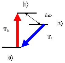
Figure 1: Three level system interacting with two heat reservoirs (hot and cold) and a quantized cavity mode.

The system is governed by the following master equation in the Schrödinger picture:

$$\mbox{\boldmath$\dot{\rho}_{mf}$}=\mathcal{L}_{h}[\mbox{\boldmath$\rho_{mf}$}]+\mathcal{L}_{dC}[\mbox{\boldmath$\rho_{mf}$}]+\mathcal{L}_{dH}[\mbox{\boldmath$\rho_{mf}$}].$$ (64)

The Hamiltonian superoperator is given by: $\mathcal{L}_{h}[\mbox{\boldmath$\rho_{mf}$}]=-\frac{i}{\hbar}[\mbox{\boldmath$H_{s}$},\mbox{\boldmath$\rho_{mf}$}]$, where $\mbox{\boldmath$H$}\equiv\mbox{\boldmath$H_{s}$}=\mbox{\boldmath$H_{m}$}+\mbox{\boldmath$H_{f}$}+\mbox{\boldmath$V_{mf}$}$ is a JCM type Hamiltonian, $\mbox{\boldmath$H_{m}$}=\hbar\bar{\sigma}\otimes\openone_{f};\ H_{f}=\hbar\omega\openone_{a}\otimes a^{{\dagger}}a;\ V_{af}=\hbar\lambda[\sigma_{21}\otimes a^{{\dagger}}+\sigma_{21}^{{\dagger}}\otimes a]$. $\mathcal{L}_{dC}[\mbox{\boldmath$\rho_{mf}$}]$ and $\mathcal{L}_{dH}[\mbox{\boldmath$\rho_{mf}$}]$ are the dissipative cold and hot Lindblad super operators, respectively:

$$\!\!\!\!\!\!\!\!\!\!\!\!\!\!\!\!\!\!\!\!\!\!\!\!\!\mathcal{L}_{dC}[\mbox{\boldmath$\rho_{mf}$}]\!\! = \!\!\Gamma_{02}\{(n_{02}\!+\!1)([\mbox{\boldmath$\sigma_{02}\rho_{mf}$},\!\mbox{\boldmath$\sigma_{02}^{{\dagger}}$}]\!+\![\mbox{\boldmath$\sigma_{02}$},\!\mbox{\boldmath$\rho_{mf}\sigma_{02}^{{\dagger}}$}])\!+\!n_{02}([\mbox{\boldmath$\sigma_{02}^{{\dagger}}\rho_{mf}$},\!\mbox{\boldmath$\sigma_{02}$}]\!+\![\mbox{\boldmath$\sigma_{02}^{{\dagger}}$},\!\mbox{\boldmath$\rho_{mf}\sigma_{02}$}])\}$$

$$\!\!\!\!\!\!\!\!\!\!\!\!\!\!\!\!\!\!\!\!\!\!\!\!\!\mathcal{L}_{dH}[\mbox{\boldmath$\rho_{mf}$}]\!\! = \!\!\Gamma_{01}\{(n_{01}\!+\!1)([\mbox{\boldmath$\sigma_{01}\rho_{mf}$},\!\mbox{\boldmath$\sigma_{01}^{{\dagger}}$}]\!+\![\mbox{\boldmath$\sigma_{01}$},\!\mbox{\boldmath$\rho_{mf}\sigma_{01}^{{\dagger}}$}])\!+\!n_{01}([\mbox{\boldmath$\sigma_{01}^{{\dagger}}\rho_{mf}$},\!\mbox{\boldmath$\sigma_{01}$}]\!+\![\mbox{\boldmath$\sigma_{01}^{{\dagger}}$},\!\mbox{\boldmath$\rho_{mf}\sigma_{01}$}])\},$$ (65)

where $\Gamma_{02}$ and $\Gamma_{01}$ are the Weiskopf-Wigner decay constant associated with the cold and hot reservoirs, respectively, and $n_{02}$ and $n_{01}$ are the number of thermal photons in the cold and hot reservoirs, respectively. The temperature of the thermal photonic reservoirs is given by:

$$T_{01(02)}=T_{H(C)}=\frac{\hbar(\omega_{1(2)}-\omega_{0})}{k_{B}\ln(1/n_{02(01)}+1)},$$ (66)

The matrix form of the matter operators is given by:

$$\sigma_{21}=\left(\begin{array}[]{ccc}0&0&0\\ 0&0&0\\ 0&1&0\end{array}\right)\ \ \ \ \ \sigma_{01}=\left(\begin{array}[]{ccc}0&1&0\\ 0&0&0\\ 0&0&0\end{array}\right)\ \ \ \ \ \sigma_{02}=\left(\begin{array}[]{ccc}0&0&1\\ 0&0&0\\ 0&0&0\end{array}\right)\ \ \ \ \ \bar{\sigma}=\left(\begin{array}[]{ccc}\omega_{0}&0&0\\ 0&\omega_{1}&0\\ 0&0&\omega_{2}\end{array}\right).$$

The extended dissipative JCM master equation (eq. 64) can be obtained by summing the Hamiltonian contribution and the two dissipative contributions. Alternatively, it can be derived in a similar fashion to the dissipative JCM master equation Erez03 . Assuming that the nature of the interaction between each pair of matter levels is dipole coupling, due to parity considerations not all three transitions would be allowed by dipole coupling. However, this issue is avoided in systems with a break in symmetry Shapiro .

Let us examine the energy flux of the matter:

$$\dot{E}_{m}=\textrm{Tr}_{m}\{\dot{\rho}_{m}H_{m}\}=-\frac{i}{\hbar}\textrm{Tr}\{\mbox{\boldmath$\rho_{mf}$}[\mbox{\boldmath$H_{m}$},\mbox{\boldmath$V_{mf}$}]\}+\textrm{Tr}\{\mathcal{L}_{d}[\mbox{\boldmath$\rho_{mf}$}]\mbox{\boldmath$H_{m}$}\},$$ (67)

where $H_{m}$ is the matter Hamiltonian without the tensor product with $\openone_{f}$. By substitution into eq. 43, heat flux and power for the matter are given by:

$$\dot{Q}_{m} = \textrm{Tr}\{\mathcal{L}_{dC}[\mbox{\boldmath$\rho_{mf}$}]\mbox{\boldmath$H_{m}$}\}+\textrm{Tr}\{\mathcal{L}_{dH}[\mbox{\boldmath$\rho_{mf}$}]\mbox{\boldmath$H_{m}$}\}=\dot{Q}_{mC}+\dot{Q}_{mH}$$

$$P_{m} = -\frac{i}{\hbar}\textrm{Tr}\{\mbox{\boldmath$\rho_{mf}$}[\mbox{\boldmath$H_{m}$},\mbox{\boldmath$V_{mf}$}]\},$$ (68)

where $\dot{Q}_{mC(H)}\equiv\textrm{Tr}\{\mathcal{L}_{dC(H)}[\mbox{\boldmath$\rho_{mf}$}]\mbox{\boldmath$H_{m}$}\}$. The energy flux of the selected cavity mode (field):

$$\dot{E}_{f}=\textrm{Tr}_{f}\{\dot{\rho}_{f}H_{f}\}=-\frac{i}{\hbar}\textrm{Tr}\{\mbox{\boldmath$\rho_{mf}$}[\mbox{\boldmath$H_{f}$},\mbox{\boldmath$V_{mf}$}]\}=P_{f},$$ (69)

where $H_{f}$ is the field Hamiltonian without the tensor product with $\openone_{m}$, and$P_{f}$ is the power associated with the field.

The energy flux of the full matter-field system is given by:

$$\dot{E}_{mf}=\textrm{Tr}\{\mathcal{L}_{dC}[\mbox{\boldmath$\rho_{mf}$}]\mbox{\boldmath$H$}\}+\textrm{Tr}\{\mathcal{L}_{dH}[\mbox{\boldmath$\rho_{mf}$}]\mbox{\boldmath$H$}\},$$ (70)

where each heat flux component is a sum of two contributions:

$$\textrm{Tr}\{\mathcal{L}_{dC(H)}[\mbox{\boldmath$\rho_{mf}$}]H\}=\textrm{Tr}\{\mathcal{L}_{dC(H)}[\mbox{\boldmath$\rho_{mf}$}](\mbox{\boldmath$H_{m}$}+\mbox{\boldmath$V_{mf}$})\}=\dot{Q}_{mC(H)}+\dot{Q}_{VC(H)},$$ (71)

where $\dot{Q}_{VC(H)}\equiv\textrm{Tr}\{\mathcal{L}_{dC(H)}[\mbox{\boldmath$\rho_{mf}$}]\mbox{\boldmath$V$}\}$. Since we are in perfect matter-field resonance, $P_{m}=-P_{f}$ ($[\mbox{\boldmath$H_{m}$},\mbox{\boldmath$V_{mf}$}]=-[\mbox{\boldmath$H_{f}$},\mbox{\boldmath$V_{mf}$}]$), hence:

$$\dot{E}_{m}+\dot{E}_{f}=\dot{E}_{mf}-\dot{Q}_{V}.$$ (72)

$\dot{Q}_{V}$ vanishes if the off-diagonal matrix elements of $\rho_{mf}$ are purely imaginary. Note that to an observer looking on the matter alone, work flux (power) and heat fluxes correspond to the traditional view of the first law of thermodynamics in which energy is divided into work and heat. The field which is the work source either receives or emits energy to the working medium (the matter) in the form of power.

In a forthcoming publication we give a full dynamical and thermodynamical analysis of the ED-JCM, and show that it acts as a quantum optical amplifier Erez03 .

IV Conclusion

In this paper we have considered the thermodynamics of unipartite systems (systems coupled to an external time dependent field and heat reservoirs), as well as bipartite systems. In the latter case, a supplementary part of the system replaces the time dependent field.

For unpartite systems, we gave a minor generalization of Alicki’s definitions for heat flux and power, by extending these definitions from the Schrödinger to the Heisenberg and interaction pictures. In this generalization, partial time derivatives replace full time derivatives in the definitions for heat flux and power. We then presented an alternative approach to the partitioning of the energy flux into heat flux and power in which the interaction energy is not included directly, that presages our bipartite treatment. We showed that at steady state, if the interaction energy contribution to the heat flux vanishes, this alternative partitioning leads to a Carnot formulation of the second law.

We then turned to bipartite systems. We presented a novel definition for power, based on the energy fluxes of the individual subsystems, that is the natural generalization of our alternative partitioning of energy flux in unipartite systems. The first law of thermodynamics was derived in differential form in two different ways. The first relies on looking at each subsystem independently, while the second relies on looking at the full bipartite system. Although any partitioning of the energy flux is consistent with the first law, the ultimate test of a good partitioning is the fulfillment of the second law. For the partitioning into (full bipartite system) + (reservoirs) the second law in the Clausius form follows almost trivially from Spohn’s entropy production function. However, for the partitioning into (subsystem A) + (subsystem B + reservoirs) we found that there is generally no second law of the Clausius type due to oscillations in the partial entropies of the subsystems. Nevertheless, at steady state both the Clausius and Carnot versions of the second law are satisfied under some well-controlled conditions. In a forthcoming publication we show, both analytically and numerically, that for the ED-JCM both the Clausius and a Carnot versions of the second law are satisfied at steady state Erez03 .

References

• (1) J. von Neumann, Mathematische Grundlagen der Quantenmechanik, Berlin: Springer (1932).
• (2) M. Born, Atomic Physics, Blackie & Son Ltd., Glasgow (1935).
• (3) R. C. Tolman, The Principles of Statistical Mechanics, Oxford University Press (1938).
• (4) H. E. D. Scovil, E. O. Schulz-DuBois, Phys. Rev. Lett. 2, 262 (1959).
• (5) E. B. Davies, Commun. Math. Phys. 39, 91 (1974).
• (6) G. Lindblad, Commun. Math. Phys. 48, 119 (1976).
• (7) G. Lindblad, Commun. Math. Phys. 40, 147 (1975).
• (8) W. Pusz, S. L. Wornowicz, Commun. Math. Phys. 58, 273 (1978).
• (9) H. Spohn, J. Math. Phys., 19, 1227 (1978).
• (10) R. Alicki, J. Phys. A 12, L103 (1979).
• (11) R. Kosloff, J. Chem. Phys. 80, 1625 (1984).
• (12) E. Geva, R. Kosloff, J. L. Skinner, J. Chem. Phys. 102, 8541 (1995).
• (13) R. Kosloff, T. Feldmann, Phys. Rev. E. 65, 055102(R) (2002).
• (14) S. Mukamel, Principles of Nonlinear Optical Spectroscopy, Oxford University Press (1995).
• (15) E. Geva, Quantum Thermodynamics in Finite Time, Ph. D. Thesis (1995).
• (16) A. Bartana, R. Kosloff, D. J. Tannor, J. Chem. Phys. 106, 1435 (1997).
• (17) E. Boukobza, D. J. Tannor, to be published.
• (18) S. J. D. Phoenix, P. L. Knight, Annals of Physics 186, 381 (1988).
• (19) E. Boukobza, D. J. Tannor, Phys. Rev. A 71, 063821 (2005).
• (20) E. T. Jaynes, F. W. Cummings, Proc. IEEE 51, 89 (1963).
• (21) P. Kral, M. Shapiro, Phys. Rev. Lett., 87, 183002 (2001).